Cosmic opacity to CMB photons and polarization measurements

Abstract

Anisotropy data analysis leaves a significant degeneracy between primeval spectral index ($n_{s}$) and cosmic opacity to CMB photons ($\tau$). Low–$l$ polarization measures, in principle, can remove it. We perform a likelihood analysis to see how cosmic variance possibly affects such a problem. We find that, for a sufficiently low noise level ($\sigma^{P}_{pix}$) and if $\tau$ is not negligibly low, the degeneracy is greatly reduced, while the residual impact of cosmic variance on $n_{s}$ and $\tau$ determinations is under control. On the contrary, if $\sigma^{P}_{pix}$ is too high, cosmic variance effects appear to be magnified. We apply general results to specific experiments and find that, if favorable conditions occur, it is possible that a 2–$\sigma$ detection of a lower limit on $\tau$ is provided by the SPOrt experiment. Furthermore, if the PLANCK experiment will measure polarization with the expected precision, the error on low–$l$ harmonics is adequate to determine $\tau$, without significant magnification of the cosmic variance. This however indicates that high sensitivity might be more important than high resolution in $\tau$ determinations. We also outline that a determination of $\tau$ is critical to perform detailed analyses on the nature of dark energy and/or on the presence of primeval gravitational waves.

&

1 Introduction

Data on cosmic microwave background (CMB) anisotropy and polarization can provide effective constraints on cosmological parameters. However, while significant anisotropy observations are available (see, e.g., Smoot et al. 1992; de Bernardis et al. 2000; Hanany et al. 2000; Halverson et al. 2002; Sievers et al. 2002; Scott et al. 2002) and further anisotropy data are expected from experiments in progress, detailed data on the weaker polarization signals may become available only within a few years. In turn, dark energy (DE) parameters or the amplitude of primeval gravitational waves (GW) are just mildly constrained by anisotropy data, while polarization would significantly depend on them. A peculiar situation then holds for the cosmic optical depth to CMB photons ($\tau$), due to reionization. Anisotropy data only mildly constrain it, while polarization data would provide more stringent constraints; of course, greater $\tau$ values would ease its detection, but, in turn, greater $\tau$ values would also ease the determination of DE and/or GW parameters.

This paper tries to investigate which polarization experiment(s) can determine $\tau$. The success of an experiment, however, will also depend on the value of $\tau$ itself. In particular, we shall consider the SPOrt experiment (Macculi et al. 2000; Carretti et al. 2000; Peverini et al. 2001), planned to perform a (nearly) full–sky polarization measure aboard of the ISS in 2004, with an angular resolution similar to COBE.

When only anisotropy data are considered, there is a degeneracy between the effects of varying $\tau$ or the primeval spectral index $n_{s}$ (Jungman et al. 1996; Zaldarriaga, Spergel & Seljak 1997; Eisenstein, Hu & Tegmark 1999; Efstathiou & Bond 1999). The most stringent limits on $\tau$, based on anisotropy data, are provided by Stompor et al. (2001), who used the outputs of recent balloon experiments to set $\tau\lesssim 0.4$ at the 2–$\sigma$ level, once $n_{s}$ is assumed $\leq 1.2$. (Such limits will be included in a number of figures here below and denominated Stompor limits). Full–sky anisotropy measures from space, like MAP or PLANCK, might improve the Stompor limits by a factor $\sim 2$. In turn, a residual uncertainty ($\sim 0.05$) on the value of $n_{s}$ is related to our scarce knowledge of $\tau$. Of course, a more precise determination of $n_{s}$ would really be welcome, first of all to shed new light on the mechanism generating primeval fluctuations. Furthermore, within a generic inflationary model, only for $n_{s}<1$ primeval GW may be expected to exist.

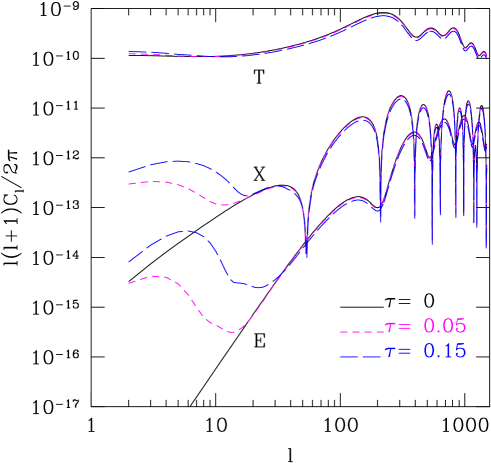
Figure 1: Angular spectra with different $\tau$ values.

The impact that a variation of $\tau$ may have on CMB polarization can be seen from Fig. 1; here, for a spatially flat cosmological model (density parameters: $\Omega_{m}=0.35$, $\Omega_{b}=0.05$; Hubble constant in units of 100 km/s/Mpc: $h=0.65$; $n_{s}=1$; dark energy is an ordinary cosmological constant) and for different values of $\tau$, we plot the dependence on $l$ of the angular spectra $C_{l}^{A}$ with $A=T,~{}E,~{}B,~{}X$, standing for anisotropy, $E$– and $B$–mode polarization and anisotropy–polarization cross correlation respectively; only $E$–mode polarization is considered through this paper. Fig. 1 shows that the main dependence on $\tau$ actually occurs at low $l$ and for the polarization and cross–correlation spectra; comparatively, the $\tau$ dependence of spectra, at $l\gtrsim 30$, is milder. This point is important to devise the right polarization experiment, which should aim to great sensitivity, while, for $\tau$ determination, high resolution data might not bear a direct relevance. Accordingly, the angular resolution of the SPOrt experiment does not prevent it from achieving cosmologically significant results.

Here, as well as in most recent literature, we assume that the whole cosmic opacity arises from an almost complete ionization of hydrogen, after a suitable redshift. More complex reionization histories may have to be taken into account to discuss future data (Bruscoli, Ferrara & Scannapieco 2002; Venkatesan 2002), but would not modify general conclusions.

For low–$l$ spectral components, varying $n_{s}$ has a milder effect than varying $\tau$. If the whole angular spectrum is considered, other parameters, like $\Omega_{tot}$, $\Omega_{m}$, $\Omega_{b}$ (total, matter and baryon density parameters), may be determined independently from low–$l$ features. Here we shall assume that they are already known from such high–$l$ anisotropy measures.

Dealing with low $l$’s, a significant part of our analysis will be devoted to inspect cosmic variance. Its impact on $C_{l}$ determination is known. Here, however, we are interested in measuring different quantities and a knowledge of $C_{l}$’s is not even required. We shall explore this point by simulating and analyzing a large number of artificial data sets. Among other things, we shall see that the SPOrt experiment, although far from granting a stringent $\tau$ determination, may improve the Stompor limit in a significant number of cases.

In the next section we shall first debate which range of values can be expected for $\tau$. We shall then describe how artificial data sets are produced. In section 4 we shall show the results of their analysis, in a number of different experimental conditions and considering different $\tau$ values. In section 5, conclusions will be drawn.

2 The cosmic opacity to CMB photons

In the present cosmic epoch, although diffuse baryonic materials are almost completely ionized, the scattering time for CMB photons $t_{s}\simeq 4.45\cdot 10^{18}\Omega_{b}^{-1}h^{-2}$s ($h$: Hubble parameter in units of 100 km/s/Mpc) exceeds the Hubble time $t_{H}=3.09\cdot 10^{17}h^{-1}$s and the Universe is transparent to CMB photons. These figures can be extrapolated to the past, but, while $t_{s}\propto a^{3}$ ($a$: the scale factor), the dependence of $t_{H}$ on $a$ depends on the cosmological model. In an expansion regime dominated by non–relativistic matter, a fully ionized Universe is opaque to CMB at $z>z_{op}\simeq 5\,(\Omega_{b}h)^{-2/3}$. Therefore, assuming $\Omega_{b}h^{2}\leq 0.022$ (standard BBNS limits; see, e.g., Dolgov 2002 for a recent review) and $h\simeq 0.5$, we have $z_{op}>64$, safely above the expected reionization redshift $z_{ri}$. No reasonable cosmological model allows a substantial reduction of such $z_{op}$.

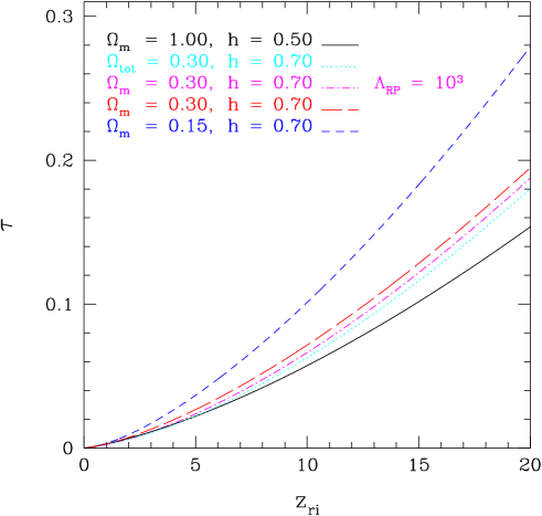
Figure 2: Dependence of $\tau$ on the reionization redshift $z_{ri}$ in various cosmological models. The only model with total density parameter $\Omega_{\rm tot}\neq 1$ is the second one. In the third model, dark energy is due to a scalar field, self–interacting through a Ratra–Peebles potential (1988), with $\Lambda_{RP}/{\rm GeV}=10^{3}$. In all models $\Omega_{b}h^{2}=0.022$. We assume (almost) all baryons to be ionized after $z_{ri}$.

On the contrary, the precise value of $\tau(\ll 1)$, does depend on the model and, in particular, on $z_{ri}$. Recent data on high–$z$ QSO’s (Djorgovski et al. 2001; Becker et al. 2001) indicate that at least a fraction of neutral hydrogen is present, in the intergalactic medium, at $z\gtrsim 6$. These very authors, however, warn us against an immediate conclusion that $z_{ri}\simeq 6$. Reionization can be a slow and/or patchy process and our present knowledge of primeval object formation can be consistent with an effective $z_{ri}\simeq 6$ or a significantly greater value. In Fig. 2 we show how $\tau$ is related to $z_{ri}$ and model features, considering a wide set of cosmological models. For $z_{ri}\lesssim 15$, values of $\tau$ up to $\sim 0.15$–0.20 are licit.

3 The artificial data sets

Artificial data sets will be built with reference to the features of the Sky Polarization Observatory (SPOrt) experiment, selected by the European Space Agency (ESA) to fly on the International Space Station (ISS) in 2004, aiming to measure the linear polarization of the diffuse sky radiation at 22, 32 and 90 GHz, using a set of polarimeters fed by corrugated horns with an angular resolution (FWHM) of $7^{o}$. At variance from other space experiments (MAP and PLANCK), SPOrt has been explicitly designed to measure the Stokes parameters Q and U and to minimize systematics and instrumental polarization. SPOrt will observe a sky area with declination $|\delta|\leq 51.6^{o}$ ($\sim 80\%$ of the whole sky). The lifetime of the experiment is at least 1.5 years, but an extension is not unlikely; data will be binned in a number of pixels ranging from 662 to several thousands, depending on the effective duration of the flight and efficiency.

In this analysis we shall assume that pixels are distributed according to the HEALPix package, with $N^{side}=8$ or 16, and smoothed with a Gaussian beam of FWHM of $7^{o}$. The two choices of $N^{side}$ allow to confirm that the best exploitation of the observational output is achieved when the average angular distance between pixel centers is $\sim$ half FWHM. For the low (high) resolution cases we shall therefore have, on the whole sky, 768 (3072) pixels, whose centers lie at an average angular distance of $\sim 7.3^{o}$ ($3.7^{o}$). Once polar caps are excluded, there remain 600 (2448) pixels, providing measures of the Stokes parameters $Q$ and $U$.

SPOrt polarimeters will provide no anisotropy data. Such information will be however available through other experiments (COBE, MAP) and we shall assume here that no peculiar problem arises in correlating SPOrt and anisotropy data. Of course, anisotropy data probe a different sky area, i.e. the whole sky, excluding the area with declination $|\delta|<20^{o}$, where galactic contamination is severe. (On the contrary, such contamination can be assumed to be under control, for polarization data; see, e.g., Bruscoli et al. 2002; Tucci et al. 2002.) For the coarse (fine) pixelization cases, as above, in this sky area there are 480 (1984) pixels. For 376 (1360) of them, both anisotropy and polarization data are supposed to be available.

Random noise ($\sigma^{P}_{pix}$) will be included in artificial data, assuming it to be uncorrelated, both among pixels and between $Q$ and $U$, in the case of polarization measures. We shall assume $\sigma^{T}_{pix}=1\,\mu$K ($2\mu$K) for temperature data (as expected for MAP measurements scaled to the SPOrt resolution). On the contrary, one of the main variables we consider is the noise level for polarization data.

SPOrt data will be characterized by $\sigma^{P}_{pix}\simeq 5.3\,{N^{side}\over 8}\,\sqrt{{1.5\over\lambda}{0.5\over\epsilon}}\,\mu$K per pixel, where $\lambda$ is the experiment’s lifetime in years while $\epsilon$ indicates the detection efficiency. Our analysis will consider $\sigma^{P}_{pix}$’s in the interval comprised from 0.5 to 5$\,\mu$K per pixel, with coarse pixelization, corresponding to 1 to 10$\,\mu$K per pixel, with fine pixelization.

The expected angular spectra $C_{l}^{T,E,B,X}$, were produced with the program CMBFAST , starting from a spatially flat cosmological model with $\Omega_{m}=0.35$, $\Omega_{b}=0.05$, $h=0.65$. Dark energy is an ordinary cosmological constant. Several values of $n_{s}$ were considered, but we shall report results only for $n_{s}=1$. Other close $n_{s}$ values yield quantitatively similar results and the potentiality of the experiment does not depend on $n_{s}$, in any appreciable way. On the contrary, our analysis aimed to exploring $\tau$ values ranging from 0.035 to 0.25. Cosmic variance was taken into account by considering 1000 independent realizations for each $\tau$ and $\sigma^{P}_{pix}$ pair.

4 Data analysis

The first aim of our analysis amounts to finding the likelihood distribution on the plane $\tau$–$n_{s}$. The number of pixels for anisotropy and polarization ($N_{T}$ and $N_{P}$) in our (artificial) data are different. Let then $T_{j}$ be the anisotropy measured in $N_{T}$ pixels and $Q_{j}$ and $U_{j}$ the Stokes parameters measured in $N_{P}$ pixels. In general, let us define vectors ${\bf x}\equiv(T_{1},.....,T_{N_{T}},Q_{1},.....,Q_{N_{P}},U_{1},.....,U_{N_{P}})$, of $N_{s}=N_{T}+2N_{P}$ components, defining an observed state of anisotropy and polarization. Once a pair of values $\tau$–$n_{s}$ is assigned, the angular spectra $C_{l}^{A}=(C_{l}^{T},C_{l}^{E},C_{l}^{X})$ are univocally determined. On the contrary, a data vector ${\bf d}$, of $N_{s}$ components, built from them, is just a realization of such model: once the $N_{s}$ component vector ${\bf d}$ is assigned, the pair of values $\tau$–$n_{s}$ is not univocally fixed.

A function

$${L}({\bf d}|C^{A}_{l})\propto[\,\det{\bf M}\,]^{-{1\over 2}}\exp\big{[}-{1\over 2}{\bf d^{T}}{\bf M}^{-1}{\bf d}\big{]}$$

shall then be built, to yield the likelihood of a given set of $C^{A}_{l}$ (i.e., of a pair of $\tau$–$n_{s}$ values), if ${\bf d}$ is observed. The main ingredient of $L$ is the correlation matrix ${\bf M_{ij}}=\langle{\bf x}^{T}_{i}{\bf x}_{j}\rangle={\bf S}_{ij}+{\bf N}_{ij}$; here ${\bf S}_{ij}$ is the signal term and ${\bf N}_{ij}$ is due to the noise. The components ${\bf M_{ij}}$ yield the correlation between the $i$th and $j$th elements of data vectors ${\bf x}$ corresponding to particular choices of $C_{l}^{A}$, i.e. of $\tau$–$n_{s}$ values. The construction of the (model dependent) signal term, however, does not require to build explicitly the vectors ${\bf x}$. The procedure to be followed, in the case when both anisotropy and polarization data are available, is explicitly reported by Zaldarriaga (1998). The construction of the noise term is simpler, as we expect no noise correlation, and the matrix ${\bf N}_{ij}=\delta_{ij}\,{\sigma_{T,pix}}^{2}$ (for $i=1,...,N_{T}$) and ${\bf N}_{ij}=\delta_{ij}\,{\sigma_{P,pix}}^{2}$ (for $i=N_{T}+1,...,N_{s}$) is diagonal.

In what follows, the technical role of the $C_{l}^{A}$ spectra will not need to be further outlined and the likelihood function will be explicitly considered to depend on $\tau$ and $n_{s}$. In particular, we assume that the most probable $\tau$–$n_{s}$ pair, for a given anisotropy–polarization state ${\bf d}$, is the one which maximizes the likelihood. On the $\tau$–$n_{s}$ plane, we can then define curves connecting points where $L$ corresponds to a given fraction of its top value. The area enclosed by each such curve corresponds to a given confidence level. In the figures below, such fractions were selected in order that the areas enclosed by the curves correspond to 68$\,\%$, 90$\,\%$ and 99$\,\%$ confidence levels. For the sake of simplicity, we shall refer to them as 1–2–3$\,\sigma$ levels.

Because of the role played by low–$l$ harmonics in our analysis, as above outlined, cosmic variance may be quite significant. Henceforth, 1000 realizations of each model will be considered; 1–2–3$\,\sigma$ curves will be obtained by averaging among the results of such realizations, so obtaining an average likelihood distribution. Of course, this is not sufficient to evaluate the expected result of a given experiment. We shall therefore implement average results with histograms, describing the distribution of results in various realizations, suitably defined for the various cases.

5 Results

Because of the large number of realizations required, we considered likelihood distributions both for coarse and fine pixelization, corresponding to distances between pixel centers of $\sim 7.3^{o}$ or $3.7^{o}$ (see section 3). A comparison of such distributions, for the cases we treated in both ways, confirms that, in general, a finer pixelization allows a better exploitation of data. Finding some general trends, however, does not require fine pixelization analysis.

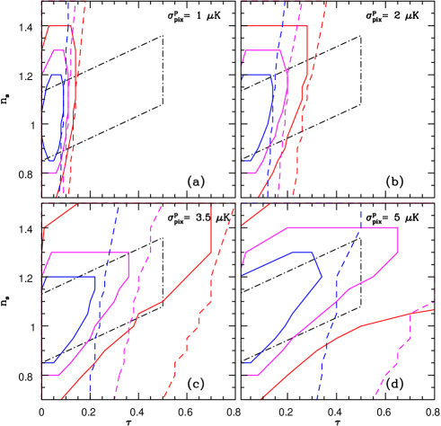
Figure 3: Average likelihood distributions, in a model with $\tau=0.05$, if the pixel–pixel angular distance is 7.3^o. Solid curves are obtained considering both anisotropy and polarization data; dashed curves are obtained with polarization data only; the corresponding confidence levels are reported in the text.

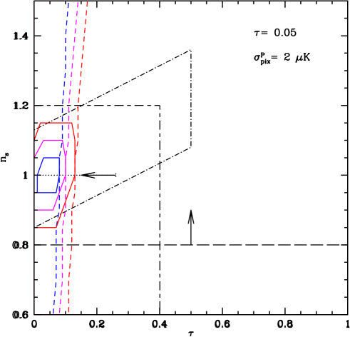
Figure 4: Average likelihood distributions, in a model with $\tau=0.05$ and $\sigma^{P}_{pix}=2\,\mu$K, if the pixel–pixel angular distance is 3.7^o. Solid and dashed curves are as in Fig. 3. The limits found by Stompor at al (2001), using anisotropy data from balloon experiments, are also shown: The dot–dashed contour limits the 95$\,\%$ confidence area, without any prior (this contour is reported in other plots as well). Assuming that $n_{s}<1.2$, they set the limit $\tau<0.4$, at the 95$\,\%$ c.l., (long–short dashed contour). With the prior $n_{s}\equiv 1$, instead, $\tau<0.26$, as shown by the arrow followed by a dotted line. Without any prior, however, they find that, at the 99$\,\%$ c.l., $n_{s}>0.8$ (long dashed line).

In Fig. 3, we report the likelihood distributions for $\tau=0.05$ and 4 levels of $\sigma^{P}_{pix}$ (for coarse pixelization). In Fig. 4, we report the likelihood distribution for the same $\tau$ value and $\sigma^{P}_{pix}=2\,\mu$K (for fine pixelization, corresponding to $1\,\mu$K with coarse pixelization). Besides of the solid curves obtained by considering both anisotropy and polarization, dashed curves are shown, obtained from polarization data only. Stompor limits are explicitly shown in Fig. 4, while in Fig. 3 we report Stompor’s 95$\,\%$ confidence limit only. See the caption of Fig. 4 for further details on Stompor limits.

From these figures it is clearly visible that upper limits on $\tau$ can be significantly improved, in respect to previous analyses, for $\sigma^{P}_{pix}\lesssim 2$–3$\,\mu$K. This is true even if only polarization data are used. The main improvement obtained, when using anisotropy data as well, concerns $n_{s}$, for which both lower and upper limits are obtained. When passing from coarse to fine pixelization, $n_{s}$ is even better constrained. If $\sigma^{P}_{pix}$ is at the lowest levels considered, $n_{s}$ determination is better than in Stompor’s case.

For what concerns lower limits on $\tau$, the situation is more critical. Detecting a lower limit, however, should be the main aim of such kind of experiments. Fig. 4 shows that a lower limit, in average, can be detected at the 1–$\sigma$ confidence level at most. This is a case, however, when average estimates themselves are insufficient. In Fig. 5, therefore, we show the distribution of 1–$\sigma$ lower limits found, with or without taking into account anisotropy, with fine pixelization. In the former case, we see that, in $\sim 78\,\%$ of cases a lower limit is found. Such percentage decreases to $\sim 70\,\%$, if no anisotropy data could be considered. For the sake of comparison, let us report that the above figures decrease to $\sim 76\,\%$ and $\sim 64\,\%$, with coarse pixelization.

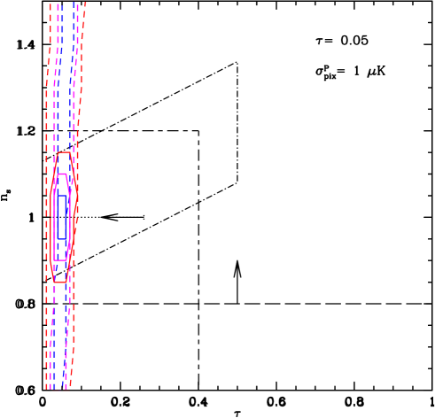
Figure 6: Average likelihood distributions, in a model with $\tau=0.05$ and $\sigma^{P}_{pix}=1\,\mu$K, if the pixel–pixel angular distance is 3.7^o. Solid and dashed curves are as in Fig. 3. This plot shows that, at this noise level, $\tau$ could be fairly reliably detected.

Going below a noise level of $2\,\mu$K per pixel (with fine pixelization), although highly problematic from an experimental point of view, would be however decisive. This is shown by Fig. 6, where we see that, for $\sigma^{P}_{pix}=1\,\mu$K, even the average 3–$\sigma$ curve indicates a detection of $\tau>0$. If the distribution of lower limits in various realizations is considered, we find that, only in $\sim 2\,\%$ of cases, no 3–$\sigma$ lower limits would be detectable.

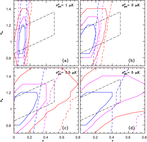
Figure 7: Average likelihood distributions, in a model with $\tau=0.10$, if the pixel–pixel angular distance is 7.3^o. Solid and dashed curves are as in Fig. 3.

Let us now consider the cases with greater $\tau$ values. They are reported in Fig. 7 and 8, for $\tau=0.10$ and 0.15. These figures are all obtained with coarse pixelization. They confirm that significant improvements of Stompor upper limits on $\tau$ are obtainable for $\sigma^{P}_{pix}\lesssim 2$–3$\,\mu$K. Moreover, lower limits become safer than in the $\tau=0.05$ case. Even with $\sigma^{P}_{pix}=2\,\mu$K, if $\tau\sim 0.15$, a 1–$\sigma$ lower limit is likely to be obtained and a 2–$\sigma$ lower limit might be obtained as well. This is an important point, as such noise levels are not far from those obtainable, in the best possible conditions, by the SPOrt experiment.

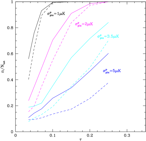
Figure 9: Fractions of realizations for which lower limits on $\tau$ are detected, at the 1–$\sigma$ confidence level, for different $\tau$ and $\sigma^{P}_{pix}$ values. Solid lines are obtained with anisotropy and polarization data. Dashed lines are obtained just with polarization. The values of $\sigma^{P}_{pix}$ reported in the plot, refer to a coarse pixelization analysis. For low values of $n/N_{tot}$, random noise causes some irregular behaviour.

It is also significant to go above average values, for lower limits, in all previous cases. In Fig. 9 to 11, we report the fractions of realizations, for which lower limits were detected, both using anisotropy–polarization data and polarization only. Among various possible comments, these plots confirm that, in order to detect $\tau$ (unless $\gtrsim 0.15$), the noise level of the SPOrt experiment is too high. It may also be significant to compare these figures with the expected noise level in the PLANCK measurements of polarization. Weighting the various channels in order to minimize variance, it is expected that $\sigma^{P}_{pix}\sim 9\,\mu$K, for a FWHM of $7^{\prime}$ (see, e.g., Hu & Okamoto 2002). If a scaling $\sigma^{P}_{pix}\propto{\rm angle}^{-1}$ is assumed, this yields $\sigma^{P}_{pix}\sim 0.4\,\mu$K, if reported to our fine pixelization. At such noise level, no magnification of the intrinsic cosmic variance seems to occur.

6 Conclusions

In this paper we performed a likelihood analysis, to determine how a polarization experiment could break the degeneracy between $n_{s}$ and $\tau$ determinations, found in pure anisotropy analyses. To this aim we built artificial data, consistent with an experiment in progress to detect polarization, but pushing noise even well below the expected experimental level. The experiment considered will cover 80$\,\%$ of the whole sky and artificial data were built assuming such sky coverage. If data were available for the full sky, a slight improvement of the signal can be expected. Artificial data were then analyzed. In respect to future observers, we have however the critical advantage to be able to analyze as many skies (realizations) we need. This is significant, in our case, as the $n_{s}$–$\tau$ degeneracy, in principle, is readily overcome from low–$l$ spectral components, where, however, cosmic variance can be critical. Our results, however, indicate that cosmic variance is not such a severe limitation, if a sufficiently low noise level is attained. This is one of the most important conclusions of our analysis, as it confirms that, to detect $\tau$, polarization experiments should aim to high sensitivity, while high resolution does not bear a direct relevance.

The critical issue, in this respect, is whether and when firm lower limits on $\tau$ are obtainable. The noise level to be attained, to implement such aim, obviously depends on the physical value of $\tau$ itself. Available constraints on $\tau$, besides that from CMB anisotropy data, can be also related to the detection of hydrogen lines in high–$z$ QSO spectra. This however leaves us a still significant range of possible cosmic opacities to CMB photons.

If $\tau$ is not negligibly low, the noise level below which we expect that lower limits on $\tau$ can be obtained is $\sigma^{P}_{\rm pix}\simeq 1$–2$\,\mu$K, for an instrument with an angular resolution similar to COBE. A detection, at higher $\sigma^{P}_{\rm pix}$, cannot be however excluded. We compared such general conclusion with the actual expected features of the SPOrt experiment and found that, for some of the greatest values for $\tau$ allowed by the cosmic reionization physics, and assuming the best possible performance of the experiment, a detection of $\tau$, at the 2–$\sigma$ level, is possible.

Acknowledgements – The public programs CMBFAST, by U. Seljak & M. Zaldarriaga, was widely used here, together with its generalization to dynamical dark energy models due to R. Mainini. The public program HEALPix, by K.M. Gòrski et al. was also widely used in the preparation of this work. Thanks are also due to Stefano Cecchini and Marco Tucci for discussions and comments.

Figure 5: Distribution of 1–$\sigma$ lower limits, for $\tau=0.05$ and $\sigma^{P}_{pix}=2\,\mu$K, if the pixel–pixel angular distance is 3.7^o. The l.h.s. (r.h.s.) plot includes (excludes) anisotropy data.

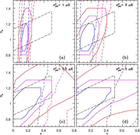
Figure 8: Average likelihood distributions, in a model with $\tau=0.15$, if the pixel–pixel angular distance is 7.3^o. Solid and dashed curves are as in Fig. 3.

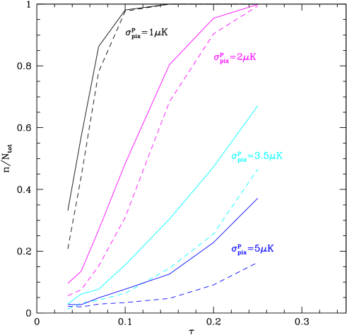
Figure 10: As Fig. 9, at the 2–$\sigma$ confidence level.

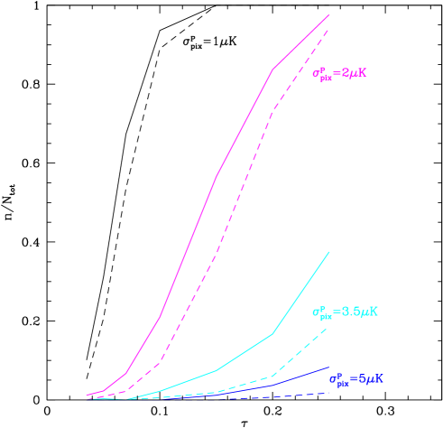
Figure 11: As Fig. 9, at the 3–$\sigma$ confidence level.

References

- [1]
- [2] [] Becker, R.H. et al., 2001, AJ, 122, 6
- [3]
- [4] [] de Bernardis, P. et al., 2000, Nature, 404, 955
- [5]
- [6] [] Bruscoli, M., Ferrara, A., & Scannapieco, E., 2002, MNRAS, 330, L43
- [7]
- [8] [] Bruscoli, M. et al., 2002, New Astr., in press, astro-ph/0202389
- [9]
- [10] [] Carretti, E., et al., 2000, in: IAU Symposium 201, New Cosmological Data and the Value of Fundamental Parameters, Astron. Soc. Pacif. Conf. Series, eds. Lasenby A. and Wilkinson A.
- [11]
- [12] [] Djorgovski, S.G., Castro, S.M., Stern, D. & Mahabal, A.A., 2001, ApJ, 560, L5
- [13]
- [14] [] Dolgov A.D., 2002, Invited Review Talk given at the VII Workshop on Topics in Astroparticle and Underground Physics (TAUP2001), Sept. 2001, L.N. Gran Sasso, Italy, astro-ph/0201107
- [15]
- [16] [] Efstathiou, G. & Bond, J.R., 1999, MNRAS, 304, 75
- [17]
- [18] [] Eisenstein, D.J., Wayne, H., & Tegmark, M., 1999, ApJ, 518, 2
- [19]
- [20] [] Hanany, S. et al., 2000, ApJ, L5
- [21]
- [22] [] Halverson, N.W. et al., 2002, ApJ, 568,38
- [23]
- [24] [] Hu, W. & Okamoto, T., 2002, ApJ, 574, 566
- [25]
- [26] [] Jungman, G., Kamionkowski, M., Kosowsky, A., & Spergel, D.N., 1996, Phys. Rev. D, 54, 1332
- [27]
- [28] [] Macculi, C., et al., 2000, in: What are the Prospect for Cosmic Physics in Italy?, eds. Aiello S. and Blanco A., Conf. Proc. 68, 171.
- [29]
- [30] [] Peverini et al., 2001, Int. Workshop on Background Polarized Emission, Bologna, 2001, AIP Conf Proc.
- [31]
- [32] [] Ratra, B. & Peebles P.J.E., 1988, Phys Rev D, 37, 3406
- [33]
- [34] [] Scott, P.F. et al., 2002, MNRAS, submitted, astro-ph/0205380
- [35]
- [36] [] Sievers, J.L. et al., 2002, astro-ph/0205387
- [37]
- [38] [] Smoot et al., 1992, ApJ, 396, L1
- [39]
- [40] [] Stompor R. et al, 2001, ApJ, 561, L7
- [41]
- [42] [] Tucci, M. et al., 2002, ApJ, in press, astro-ph/0207273
- [43]
- [44] [] Venkatesan, A., 2002, ApJ, 572, 15
- [45]
- [46] [] Zaldarriaga, M., Spergel, D.N., & Seljak, U., 1997, ApJ, 488, 1
- [47]
- [48] [] Zaldarriaga, M., 1998, ApJ, 503
- [49]