Inferring physical conditions in interstellar clouds of H₂

Abstract

We have developed a code that models the formation, destruction, radiative transfer, and vibrational/rotational excitation of H₂ in a detailed fashion. We discuss generally how such codes, together with FUSE observations of H₂ in diffuse and translucent lines of sight, may be used to infer various physical parameters. We illustrate the effects of changes in the major physical parameters (UV radiation field, gas density, metallicity), and we point out the extent to which changes in one parameter may be mirrored by changes in another. We provide an analytic formula for the molecular fraction, f_H2, as a function of cloud column density, radiation fields, and grain formation rate of of H₂. Some diffuse and translucent lines of sight may be concatenations of multiple distinct clouds viewed together. Such situations can give rise to observables that agree with the data, complicating the problem of uniquely identifying one set of physical parameters with a line of sight. Finally, we illustrate the application of our code to an ensemble of data, such as our FUSE survey of H₂ in the Large and Small Magellanic Clouds (LMC/SMC), in order to constrain the elevated UV radiation field intensity and reduced grain formation rate of H₂ in those low-metallicity environments.

1 Introduction

1.1 Overview

No molecule in astrophysics is as ubiquitous or as far-reaching in its effects as molecular hydrogen (H₂). Found in nearly every physical environment and in every temporal domain, it was the first neutral molecule to form after the Big Bang, it is a major constituent of giant molecular clouds, and it forms the bulk of the atmospheres of Jovian planets. Of particular relevance to our interests is the fact that H₂ is the most abundant molecule in the interstellar medium (ISM); nearly every target through the Galactic disk and halo observed with the Far Ultraviolet Spectrographic Explorer (FUSE) since its launch in June 1999 has exhibited signs of H₂ along the line of sight (Shull et al. 2000). Studying H₂ is a major scientific goal of FUSE; in addition to the diffuse cloud program, nearing completion with $\sim$ 100 targets in the Galactic disk, active FUSE campaigns exist to study H₂ in the LMC/SMC (Tumlinson et al. 2002) and in denser “translucent” clouds having a visual extinction in the range of about $A_{V}=1\rightarrow 5$ (Snow et al. 2000; Rachford et al. 2001). Thoroughly understanding such clouds of H₂, which are the raw ingredients out of which giant molecular clouds and, later, stars form could lead to better comprehension of that process or the physical nature of the ISM in general.

Here, we discuss new computational models of interstellar clouds of H₂ and their application to FUSE data. Information on the theory and construction of these models, a summary of their application to large FUSE datasets, and interpretations of the results form the bulk of this paper.

1.2 Background material

A brief reminder of the physics of the H₂ molecule is in order. Molecular hydrogen has quantized electronic, vibrational, and rotational degrees of freedom, giving rise to a commensurate set of energy levels. The ground electronic state ($X^{1}\Sigma_{g}^{+}$) is split into a number of vibrational levels (labeled $v=0,1,...,14$), which are in turn split into rotational levels ($J=0,1,...$). Higher electronic states (the next two of singlet symmetry are labeled $B^{1}\Sigma_{u}^{+}$ and $C^{1}\Pi_{u}$) are also split into vibrational and rotational levels, and absorptions from the ground state into these electronic states are referred to as the Lyman ($B^{1}\Sigma_{u}^{+}\leftarrow X^{1}\Sigma_{g}^{+}$) or Werner ($C^{1}\Pi_{u}\leftarrow X^{1}\Sigma_{g}^{+}$) bands. Molecular hydrogen in its ground electronic state has no permanent electric dipole moment, and hence no dipole-allowed vibrational or rotational transitions. Consequently, cold H₂ is most readily detected via observation of its ultraviolet absorption in these electronic bands (Shull & Beckwith 1982).

The Lyman and Werner bands occur in the far-ultraviolet portion of the spectrum, and so their observation is entirely the purview of space-based missions. Early efforts in this vein (see Snow 2000, and references therein) included rocket-borne spectrographs (e.g., Carruthers 1967), the Copernicus mission, the Interstellar Medium Absorption Profile Spectrograph, the ORFEUS spectrograph, and the Hopkins Ultraviolet Telescope. The data we consider here are from FUSE – the most recent mission capable of attacking this problem – the details of which are described in Moos et al. (2000) and Sahnow et al. (2000). FUSE is a multi-channel Rowland circle spectrograph, with coverage of the spectral range from approximately 912 to 1187 Å  and a spectral resolution of approximately $R=20,000$. It is FUSE’s ability to measure accurate column densities in rotational and vibrational levels that makes possible the detailed analysis of diffuse and translucent lines of sight described here.

2 Modeling H₂

2.1 Overview

The modeling process itself is principally a game of balance. In a steady state, those processes that populate a level must balance those that depopulate it. In the larger sense, there also exists a balance between formation of the molecule on grains and its destruction, primarily via absorption in the Lyman or Werner bands, followed by decay approximately $11\%$ of the time to the vibrational continuum of the ground electronic state. The primary population mechanisms are spontaneous radiative decay from higher levels, cascades from upper levels following absorption in the Lyman or Werner bands, direct formation into the level, and collisional excitation. The primary depopulation schemes of rotational states $J\geq 2$ in the ground vibrational level, for the conditions prevalent in the ISM, are radiative absorption out of a given level, spontaneous radiative decay, and collisional de-excitation. At low temperatures, only reactive collisions with charged particles (H⁺, H${}_{3}^{+}$) couple odd-$J$ (ortho) and even-$J$ (para) H₂, which otherwise behave as separate species. Absorption in the Lyman and Werner lines varies with depth in the cloud, as these lines become “self-shielded”; this results in decreased photo-destruction rates. Finding the steady-state level populations at each point in a cloud is then a matter of determining the magnitude of all these effects, and then solving the system of equations for the resulting $n(v,J)$, the physical density in each rotational, vibrational level.

The first attempts to model clouds in this fashion were carried out by Black & Dalgarno (1973). Many later efforts in the same vein (Spitzer & Zweibel 1974; Jura 1975a, Jura 1975b; Black & Dalgarno 1976, 1977; Shull 1978; van Dishoeck & Black 1986, hereafter vDB; Black & van Dishoeck 1987; Sternberg 1988; Sternberg & Dalgarno 1989; Draine & Bertoldi 1996) have followed basically this prescription, with some variations in the processes taken into account, the rates used for collisional and radiative processes, and the approximations made.

We have developed a C++ code that performs the analysis described above. Its treatment of the radiative transfer in the Lyman and Werner lines is reasonably sophisticated. Rather than relying on analytical or “equivalent width” approximations to the attenuation at each depth step, we simulate the clouds as isothermal slabs with an ambient radiation field incident on one or two sides. We carry out numerical integrations over full Voigt line profiles to calculate the absorption out of each $(v,J)$ level at each of typically 500 depth steps. (In the case where clouds are illuminated on two sides, an iterative procedure is used to solve for the radiation field at each depth step.) A major advantage of this technique is that it allows us to account in an accurate and natural fashion for line overlap, expected to be of special importance in the high-column-density translucent systems. Figure 1, taken from FUSE observations of five different targets, shows how serious line overlap can be, as $N(H_{2})$ approaches 10²¹ cm^-2. This procedure also provides us with a simulated absorption spectrum at every depth step in the cloud, which provides a graphical check to the physical modeling.

Figure 2 shows a sample of simulated spectra at two different depths in a cloud of physical density of hydrogen nuclei $n_{H}=70$ cm^-3 and temperature $T=98$ K. The dashed line in this figure corresponds to a depth in the cloud where the total H₂ column is $1.2\times 10^{20}$ cm^-2; the solid line corresponds to $1.2\times 10^{16}$ cm^-2. The primary result of a model such as this is a set of physical densities $n(v,J)$ at every depth in the cloud, which can be integrated through the cloud to provide a column density $N(v,J)$, in turn comparable with FUSE observations. For completeness, we note that the rates for collisional and radiative processes employed in our models differ (in some cases appreciably) from those used in some previous models, owing to more recent and sophisticated quantum-mechanical calculations of those rates. For radiative rates, we use the work of Wolniewicz, Simbotin, & Dalgarno (1998) and Abgrall et al. (1994); collisional rates for H₂-H and H₂-H₂ interactions are from Le Bourlot et al. (1999). Proton-H₂ collision rates are from Dalgarno, Black, & Weisheit (1973), and Gerlich (1990); the former’s rate for the $J=1\rightarrow 0$ transition is, for computational reasons, used for the large grids of models discussed below, but this has negligible effect on the resulting $N(J)$. We treat H⁺ as a species with fixed abundance, $n_{H+}/n_{H}=10^{-4}$, and assume a cosmic-ray ionizing frequency of $2\times 10^{-17}$ s^-1. We assume a Doppler line-broadening parameter $b=5$ km s^-1 in all the models discussed here.

In Table 1, we compare a set of reference models, computed using our code, to other models in the literature (vDB). The models from the literature have fixed $N(H_{2})$; to match roughly these total $N(H_{2})$, the comparison models using our code were run with $r=1.33$ pc. Models in this table have $n_{H}=250$ cm^-3, $I=2\times 10^{-8}$ photons cm^-2 s^-1 Hz^-1, and $T=$ 20, 40, 60, 100 K, to match models C1, C4, C7, and C10 in vDB. While we do not obtain precisely the same $N(J)$ as vDB for a given set of physical conditions, the differences between our results are $<$ 20 % in most cases. These discrepancies are probably attributable to our different treatment of the radiative transfer, coupled with different values for the collisional and radiative rates involved in these calculations.

We wish to keep the models relatively well-constrained by the data, in order to examine what happens when basic physical parameters like temperature, density, and UV radiation field are altered. Therefore, we have chosen to make a number of simplifications to the modeling process. The remainder of this section is devoted to highlighting and discussing some of these approximations.

2.2 Isothermality

Our models have constant physical temperature and total physical density. This is clearly an idealization, and for larger clouds it is probably a poor one, but we see no clearly superior and viable characterization of the diffuse clouds we observe. While polytropic equations of state have been used to model interstellar clouds (e.g., vDB), and appear to be a reasonable approximation to their structure, they are not appropriate for our purposes here. Modeling clouds as polytropes introduces additional parameters that cannot be regarded as fixed by observations; it also obscures one of our central goals, to determine what happens to observational diagnostics of these clouds as basic physical parameters are changed. Also, some of the diffuse clouds discussed here may be so far from a pressure-bounded equilibrium that polytropes would be inappropriate as a description of their structure. While such clouds are also unlikely to be isothermal, nor even indeed truly amenable to the steady-state modeling performed here, it is natural to model them first with as simple a parameterization as possible. Other schemes in which temperature and density vary – e.g. a “constant pressure” model where the product $nT$ is held constant – might also be potentially appropriate descriptions of these structures, but no strong constraints on the temperature and density distributions exist. Although an ad hoc distribution might provide a good match to some of the data, it is too ill-constrained to be of serious use.

We have not attempted to solve for the thermal balance of the clouds self-consistently, because it would be computationally intensive and because some facets of the thermal balance problem are not well understood. In particular, the photoelectric effect on dust grains is probably a major heating source for the gas (Wolfire et al. 1995; Boulanger et al. 2000), but the details of that heating mechanism for a given physical environment are poorly constrained. Leaving temperature as a free parameter also allows us to explore what will happen to the H₂ in clouds where the gas is anomalously heated (by, e.g., thermal shocks or MHD wave-damping).

2.3 The Slab Geometry

We simulate the clouds as slabs with a radiation field incident on one or two sides; this is also clearly an idealization. Interstellar clouds are rarely slabs, but again it is not entirely clear how one might improve on this picture without vastly exceeding our ability to constrain it. Representing the clouds as spheres rather than slabs might more closely approximate their true nature, but it is appreciably more difficult computationally. Such a representation also seems to us unlikely to change qualitatively the nature of our results here, so we have not undertaken it. The slab approximation means that we are probably underestimating the radiation field at points interior to the cloud, since presumably the real clouds are finite in directions perpendicular to the line of sight, and therefore admit some radiation from those directions. This additional radiation input, however, should be small in most cases; qualitatively, we expect the additional radiation to be comparable to that coming from the “far side” of a two-sided slab. To estimate this effect, we point out Table 2, which shows column densities, $N(J)$, for an arbitrary model, calculated using both one and two-sided slab approximations. The additional radiation input provided by the far side has the expected effect of boosting the higher-$J$ levels slightly, but the effect is modest (less than $\sim$ 0.3 dex in $N(J)$ for all models calculated under both schemes).

2.4 Radiative Transfer Issues

We assume that the line and continuum attenuations of the radiation field are separable, and we incorporate dust into the continuum attenuation. We assume the dust model of Roberge et al. (1981), which is a forward-scattering grain model. This choice of model has previously been shown to have relatively little effect on the H₂ population (vDB). The radiation field at each depth in the cloud is discretized on a large grid of frequency points. The total attenuation at each depth is calculated at all of those frequency points by considering the contribution to the total absorption cross-section from every line in the Lyman and Werner bands, together with the continuum attenuation.

The radiation fields that illuminate our model clouds are flat in photon space between 912 and 1120 Å, e.g. $I_{\nu}=2\times 10^{-8}$ photons cm^-2 s^-1 Hz^-1. The actual Galactic far-UV spectrum varies somewhat across the wavelengths relevant here. However, we have chosen not to include this variation as input to the models, because for some of the environments considered here (e.g., the low-metallicity LMC and SMC, or Galactic clouds exposed to high radiation field), a Galactic spectrum is probably inappropriate. In Table 3, we compare a representative model with a flat spectrum, $I_{\nu}=$ 2 $\times 10^{-8}$ photons cm^-2 s^-1 Hz^-1, against one with an incident spectrum of UV radiation designed to approximate more closely UV starlight (Draine 1978),

$$\lambda u_{\lambda}=(4\times 10^{-14}{\rm\ ergs\ cm}^{-3})\ \chi\lambda_{3}^{-5}(31.016\lambda_{3}^{2}-49.913\lambda_{3}+19.897)$$ (1)

with $\chi=1.71$ and where $\lambda_{3}=\lambda/10^{3}$ Å. The level populations of models exposed to these different UV radiation fields are not identical, but the differences are small relative to those discussed in the analysis of data below. Note that while we refer here to a spectrum of $I=$ 1 $\times 10^{-8}$ photons cm^-2 s^-1 Hz^-1 as a rough “Galactic mean” UV radiation field, the column densities for clouds exposed to the Draine (1978) radiation field are closest to those with a flat spectrum somewhere in the range $I=$ (2-3) $\times 10^{-8}$ photons cm^-2 s^-1 Hz^-1.

2.5 Formation Process

In the conditions prevalent in the ISM, H₂ is believed to form primarily on the surfaces of dust grains (Hollenbach, Werner, & Salpeter 1971). While a few details of this process remain unclear (see Herbst 2000), the basic scheme is that formation proceeds when an H atom collides with a dust grain, is adsorbed and moves across the grain surface, encounters a previously adsorbed H atom on the grain, recombines, and pops off the grain. Much recent work has provided new insights into the details of this formation process (e.g., Katz et al. 1999), although these turn out to be largely irrelevant to our results – see below. In principle, the rate at which formation on grains occurs is a function of the grain size, abundance, gas and grain temperature, and sticking factor. Here, we express the grain formation rate per H atom as a constant $R$ (in cm³ s^-1), which is a free parameter in the models; that is, we suppress explicit independent variation of all the different quantities that affect the overall rate. The volume rate of formation on grain surfaces is then $n_{H}n_{HI}R$, where $R\approx 3\times 10^{-17}$ cm³ s^-1 for Galactic conditions (Hollenbach, Werner, & Salpeter 1971; Jura 1974).

3 Determining physical parameters

3.1 Overview

In the sections that follow, we apply our code to the problem of determining how changes in physical conditions along a line of sight affect observed column densities. To do so, we have created a large ($>$ 5000 element) grid of models of varying temperature, density, size, UV radiation field, and grain formation rate of H₂. Here, we examine how changes in these major physical parameters are manifested in various diagnostics, and we give scaling relations which approximate the quantitative changes in molecular fraction incurred by altering the radiation field or grain formation rate.

3.2 Diagnostics

Many different quantities might in principle act as comparators between the data and attempts to model them. The measured column densities themselves can of course be compared to calculated ones, but they do not by themselves serve as reliable indicators of physical parameters like density, temperature, and UV radiation field; direct comparison of column densities is also unwieldy for large datasets. In this section, we give a brief overview of the additional diagnostics we have chosen, and the reasons why we have chosen them.

One such diagnostic is the fraction of hydrogen nuclei in molecular form,

$$f_{H2}=\frac{2N(H_{2})}{[N(HI)+2N(H_{2})]}.$$ (2)

In the standard simple model of an interstellar cloud (Jura 1975a,b), as described above and implemented in our code, H₂ is assumed to be in equilibrium between formation on grains with rate coefficient $R$ (cm³ s^-1) and photodestruction with rate $D$ (s^-1),

$$Dn(H_{2})=Rn_{H}n_{HI}\approx 0.11\sum_{J}\beta(J)n(H_{2},J).$$ (3)

Here, we have assumed that the fraction of absorptions which lead to dissociation, $f_{diss}$, is 0.11. In the code, we do not make this assumption, but explicitly calculate $f_{diss}$ for each band. It varies somewhat, depending on the radiation field and depth into the cloud, but always lies in the range 0.10 – 0.15.

If one assumes that the cloud is homogeneous, with physical densities replaced by column densities, then one may relate $f_{H2}$, as defined above, to the formation and photodestruction rates :

$$f_{H2}=\frac{2Rn_{H}}{D}.$$ (4)

Thus, the molecular fraction can be suppressed either by a depressed formation rate or an enhanced photodestruction rate. Qualitatively, $f_{H2}$ acts as measure of the balance between these two processes.

To probe the temperature of the gas, one typically turns to the excitation temperature describing the populations of $J=0$ and $J=1$, given by

$$T_{01}=\frac{(\Delta E_{01})/k}{\ln[(g_{1}/g_{0})N(0)/N(1)]},$$ (5)

where $g_{1}/g_{0}=9$ is the ratio of statistical weights of the $J=1$ and $J=0$ levels, and $(\Delta E_{01})/k=171$ K. At densities high enough for collisions with H⁺ and H${}_{3}^{+}$ to dominate the (0,1) level populations (such as in the translucent clouds), $T_{01}$ must trace the kinetic temperature. At the densities typical of diffuse clouds, the relation between these two quantities is not precisely known (Tumlinson et al. 2002), but $T_{01}$ probably still traces $T_{kin}$ to some extent for $N(H_{2})\geq 10^{16}$ cm^-2. The kinetic temperature is a free parameter in our models.

One can construct similar excitation temperatures, or equivalent quantities, for any two levels. However, these are decreasingly sensitive to the kinetic temperature and increasingly sensitive to details of the radiative cascade as one goes to increasing $J$. In particular, we employ the column density ratios N(3)/N(1), N(4)/N(2), and N(5)/N(3). The first ratio is probably still sensitive to collisional processes in the gas (Jura 1975b; Tumlinson et al. 2002), but the latter two ratios likely probe the radiation field rather than the kinetics of the gas.

One caveat to the use of column density ratios is that, while these ratios can be a useful diagnostic of the radiation field (and potentially of the thermal structure along a line of sight), they do represent a loss of information relative to the individual column densities. It is possible for two sightlines to have very similar column density ratios but very different actual column densities.

By examining all of these diagnostics together, we can assess quantitatively the overall abundance of H₂ and its excitation, in both models and data.

3.3 Thermal effects

In Figure 3, we show two sets of models with a range of densities and sizes (such that $N(H_{2})$ $<9.0\times 10^{21}$ cm^-2), but with constant (and high) UV radiation field, $I=5\times 10^{-7}$ photons cm^-2 s^-1 Hz^-1, about 50 times the Galactic mean. The models shown as triangles are at a kinetic temperature $T=10$ K, while those shown as diamonds are at $T=90$ K. Also shown are “trend lines” connecting corresponding points in the two models; these indicate how points in the excitation diagram move in response to decreasing temperature. In general, decreasing the kinetic temperature for clouds with $N(H_{2})$ $\gtrsim$ 10²⁰ cm^-2 moves points towards higher excitation ratios N(4)/N(2) and N(5)/N(3). This is largely a result of the fact that, at these temperatures, $J=4$ and $J=5$ are not populated to a signficant extent by collisional processes, but rather by radiative cascade. Although collisions indirectly modify the $J=4$ and $J=5$ populations, this effect is small. The population of $J=2$, however, is more directly affected by collisional processes, albeit on a still-minor level. Thus, as the kinetic temperature drops, a population source for $J=2$ disappears, while the population sources of $J=4$ and higher do not. This effect is only noticeable when collisional effects are significant relative to radiative ones for $J=2$, so at low column densities, where incident radiation is less shielded, changing the temperature has little effect on the excitation ratios. At intermediate column densities, where collisional population of $J=2$ is negligible but collisional population of $J=1$ is not, changes in temperature can have the opposite effect on excitation. As the temperature rises in this regime, $J=1$ is populated at the expense of $J=0$, thus reducing slightly the population rate via radiative cascade for both $J=2$ and $J=4$. The small difference in physical density affects the column density of $J=2$ more strongly than it does $J=4$, since the former level is beginning to self-shield while the latter does not. Thus, for column densities $N(H_{2})$ between roughly 10¹⁷ cm^-2 and 10²⁰ cm^-2, increases in kinetic temperature translate to increases in the excitation ratio N(4)/N(2).

A minor complication in these analyses is that changing the temperature can slightly affect the total $N(H_{2})$. As the temperature drops, all other things being equal, more material will reside in the lowest rotational level, $J=0$. This means that $J=0$ will become strongly self-shielding earlier, depressing the photo-destruction rate further into the cloud, and the total abundance of H₂ will rise slightly. This effect is only important in the critical regime where absorption out of $J=0$ is not already highly damped; at higher column densities, a small increase in the population of $J=0$ has no appreciable affect on the total photodestruction rate and, hence, on the total molecular abundance.

3.4 UV radiation field

As the UV radiation field becomes stronger, the photo-destruction rate clearly also rises; hence, a first-order effect of the enhanced radiation field is to lower the molecular fraction. This effect is displayed in the top left panel of Figure 4, which shows molecular fractions for models at the same density and temperature but different radiation fields. As seen here, an enhanced radiation field also has the effect of delaying the onset of very high molecular fraction, since the higher rate of UV absorption means that the major absorption lines out of $J=0$ and $J=1$ become optically thick at larger $N_{H}$. Thus, the critical regime where small changes in column density correspond to large changes in $f_{H2}$ also occurs at higher $N(H_{2})$. A high UV radiation field can also change fairly dramatically the ratios of the populations in each rotational-vibrational level. The bottom left panel of Figure 4 shows the excitation ratio N(4)/N(2) for models at the same temperature ($T=60$ K) and density ($n_{H}$ = 100 cm^-3), but with two different UV radiation fields. Models in green are exposed to a field roughly the Galactic mean, $I=1\times 10^{-8}$ photons cm^-2 s^-1 Hz^-1; models in red are exposed to a field 50 times as intense. At lower radiation field intensities, a disparity quickly arises between levels $J=0$ and $J=1$ on the one hand, and all higher levels on the other. Because these two lowest levels have no means for spontaneous de-excitation, absorption lines out of those levels become damped. The rates out of these levels deep in the cloud become smaller by a factor $\sim 100$ compared to values at the edge of cloud. Higher levels, on the other hand, have spontaneous deexcitation probabilities that can quickly become the dominant means for depopulating the level. The primary population mechanism (radiative absorption and subsequent cascade into the given level) is not strongly biased towards any one level or set of levels. Thus, $J=0$ and $J=1$ become a “sink” for H₂ relative to the other levels, with the relative magnitudes of the level populations set largely by the ratio of the dominant depopulation mechanisms (spontaneous radiative decay for $J\geq$ 2, highly damped absorption for $J=0$ and $J=1$).

3.5 Grain formation rate

Changes in the grain formation rate also clearly affect the molecular fraction. As less H₂ is formed on grains, all other things being equal, the molecular fraction must drop. In the top right panel of Figure 4, we show the effects on molecular fraction of reducing the grain formation rate coefficient of H₂ by a factor of ten; in this figure, all clouds are exposed to a Galactic mean radiation field and have the same temperature ($T=90$ K).

The effect on excitation ratios is, again, more subtle. In the bottom right panel of Figure 4, we show the excitation ratio N(4)/N(2) for models exposed to the same Galactic mean radiation field, but with grain formation rates which differ by a factor of ten. Changes in the grain formation rate can affect the ratios of column densities in each ro-vibrational level by changing the total column density of H₂ for a given physical density, radiation field, and temperature. This change leads to more or less damping of absorption in the $J=0$ and $J=1$ Lyman and Werner bands, and can therefore alter the level populations. In general, decreasing the grain formation rate enhances the excitation ratio N(4)/N(2), but does not appreciably alter the ratio N(5)/N(3).

As before, changes in both the total molecular abundance and in the excitation ratios are most pronounced for clouds that lie on the cusp of self-shielding (i.e., those with $N(H_{2})$ $\sim 10^{18}$ cm^-2).

3.6 Scaling relation

Here, we give an approximate relation for the molecular fraction in a cloud of H₂ as a function of the total hydrogen column density, $N_{H}$, the grain formation rate of H₂, and the intensity of the UV radiation field. This relation is intended to be most accurate for conditions approaching nominal Galactic ones; for environments with radiation fields or grain formation rates far away from the Galactic ones, it is only a rough approximation. In general, we consider a relationship of the type

$$\log(f_{H2})=A_{0}q\left[1-0.98\tanh\left(\frac{\log(N_{H})-A_{1}q}{A_{2}q}\right)\right],$$ (6)

where

$$q=\alpha(R)\beta(I)=\left(\frac{R}{R_{0}}\right)^{A_{3}}\left(\frac{I}{I_{0}}\right)^{A_{4}},$$ (7)

and we take $I_{0}=10^{-8}$ photons cm² s^-1 Hz^-1 and $R_{0}=3\times 10^{-17}$ cm³ s^-1. This functional form was chosen because it has the property of going from a low value ($\sim 2A_{0}$, where $A_{0}$ is a negative number) to a high one ($\sim 0.98$, equivalent to the highest molecular fraction reached by model clouds in this sample) at a characteristic column density set by the value of $A_{1}$ and over a scale set by $A_{2}$. The parameter $q$, a proxy for the two independent parameters $A_{3}$ and $A_{4}$, expresses variation in $R$ and $I$. Including the variations with respect to $R$ and $I$ makes this a four-parameter fit; allowing the dependence on $R$ and $I$ to vary in each of the terms in this equation does not improve the fit.

The best-fit values were obtained by performing multi-dimensional parameter minimizations against the results derived from the model cloud grid. We find $A_{0}=-2.4054$, $A_{1}=20.178$, $A_{2}=0.279$, $A_{3}=-0.0118$, and $A_{4}=0.0124$. In the leftmost panel of Figure 5, we show model clouds with roughly Galactic radiation field ($I_{0}$) and grain formation rate ($R_{0}$) together with this scaling relation; the agreement here is good at all points. Some small vertical scatter in the molecular fractions of model points is caused by the spread of temperatures in the models and accompanying small changes in the molecular content of the gas (discussed above). We have not included any variation with respect to temperature in the scaling relation given here, because it is generally much smaller than the effects induced by changing other quantities. In the middle panel of Figure 5, we show models exposed to a Galactic radiation field but at a range of grain formation rates down to one-tenth the Galactic mean. The agreement with the scaling relation is generally good, but begins to degrade at low molecular fractions and low $N_{H}$. In the rightmost panel of Figure 5, we include models exposed to a radiation field of up to $I=1\times 10^{-7}$ photons cm^-2 s^-1 Hz^-1. Here, the agreement with the data is fairly poor at very low molecular fractions ($f_{H2}\lesssim 10^{-5}$) but good at higher ones; the scaling relation given here overestimates the molecular fraction in highly optically thin clouds. This problem persists at even higher radiation fields. Thus, this scaling relation cannot be used as a substitute for detailed modeling in environments far removed from the nominal Galactic one. It can, however, give an order-of-magnitude estimate for the molecular fraction in such environments, and under Galactic conditions it can be used in a more precise fashion.

We can find no such simple scaling relation for the excitation ratios N(4)/N(2) and N(5)/N(3); too many effects combine to yield the observed ratios for them to be easily described throughout the parameter space considered here.

4 The translucent cloud paradigm

In general, while the simple models we have presented here can duplicate most diffuse cloud observations, they cannot match the observed populations of very high-$N(H_{2})$ clouds ($N(H_{2})$ $\gtrsim 10^{20}$ cm^-2) without supposing rather high incident UV radiation fields ($\gtrsim 20\times$ Galactic mean). This may be appropriate in some cases, but probably not all. In addition, some of the observed high-column cloud populations cannot be explained by the isothermal slab models at all. In a single slab, it is difficult to populate the rotational states $J>4$ to the levels observed in these targets without vastly overpopulating the lower-$J$ states.

We suggest that some high-$N(H_{2})$ clouds are combinations of lower-$N(H_{2})$ diffuse clouds viewed along a common line of sight. We do not refer here to the idea of having a “shell” model for a cloud, wherein a single line of sight consists of a monolithic object with one hot exterior region and one cool interior. Some lines of sight may indeed have this sort of structure, but we also suggest the possibility of physically distinct clouds, each exposed to an incident radiation field that is not filtered through the other component clouds. This interpretation is appealing in part because of the results from single-component analyses, in which high radiation fields are necessary to match any of the high-$N(H_{2})$ line of sight observations. If intense incident radiation fields are not a possibility for a given line of sight, then there must be additional pathways by which UV radiation is entering the system (c.f. Rachford et al. 2001). For a given incident radiation field, one way of enhancing the effect of that radiation field (and hence bringing the model clouds into agreement with observations) is to allow it to enter the system at multiple points, so it is not completely attenuated far into the cloud.

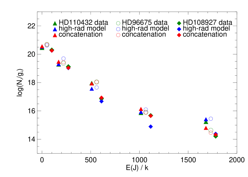
Figure 6: Populations $N(J)$ vs. rotational energy E(J), for three high-$N(H_{2})$ sightlines, together with both single-cloud and two-component models. Each sightline is represented by a different symbol; triangles correspond to HD 110432, circles to HD 96675, and diamonds to HD 108927. Green, blue, and red points correspond, for each target, to data, high radiation field model, and concatenation model respectively. The sightlines have been displaced slightly along the $x$ axis for clarity. See text for discussion.

In Figure 6, we show H₂ observations along three selected high-$N(H_{2})$ lines of sight : HD 108927 and HD 96675 (Gry et al. 2002), and HD 110432 (Rachford et al. 2001). For each line of sight, two model calculations are also shown – one that is the best single-cloud match to the data, and another, which is a concatenation of two clouds. Out of the many possible concatenations that can match the data, we have chosen the best match for which both component clouds are illuminated by a radiation field of no more than $4\times 10^{-8}$ photons cm^-2 s^-1 Hz^-1, about four times the Galactic mean. In these two-cloud models, one cool component contributes most of the total column density of H₂, while the other component, smaller and hotter ($\sim 200$ K), helps populate the high-$J$ states. The single-cloud matches are all exposed to a high radiation field ($\gtrsim 2\times 10^{-7}$ photons cm^-2 s^-1 Hz^-1), not because we have excluded lower radiation field matches but because all individual models in our database that can match the observed populations are exposed to such high fields.

We have thus far been wary of describing these three sightlines as “translucent clouds,” because only two out of the three (HD 110432 and HD 96675) meet the defining requirement that the visual extinction $A_{V}>1$. (The remaining target considered here, HD 108927, has $A_{V}\approx 0.68\pm 0.1$.) While the visual extinction may indeed be an important discriminator of cloud properties (Rachford et al. 2001), there does not seem to be a crucial difference between clouds with $A_{V}=1-2$ and those with slightly lower extinction. All three clouds share the common property that multiple radiation pathways (or a very high radiation field) are required to explain their observed populations. A more fundamental distinction between “diffuse” and “translucent” clouds may be one of molecular fraction: in models of all three sightlines, one component cloud must have a fairly high molecular fraction ($f_{H2}\gtrsim 0.5$), in sharp contrast to the very low molecular fractions ($f_{H2}\sim 10^{-5}$) observed in many model clouds with $\log(N_{H})\lesssim 21.25$ (for Galactic grain formation rate and UV radiation field). One difficulty with such a definition, however, is that the molecular fraction is generally not known along sightlines with high $N(H_{2})$; to estimate it, one uses an assumed relationship between the observed color excess and the total N_H. We also note that very high extinction clouds with A_V $\gtrsim 5$ may be very different from the clouds considered here, but such high-extinction clouds cannot be studied by FUSE because of the low FUV fluxes of background stars.

Another high-$N(H_{2})$ sightline, towards HD 73882 (Snow et al. 2000; Ferlet et al. 2000), is not well-matched by a two-cloud concatenation where neither absorber is exposed to a high radiation field as described above. It is also not well-matched by any single cloud in our model database, regardless of radiation field. For these reasons, we have not included it in Figure 6. It is possible that the absorbers towards HD 73882 (spectral type O8.5) are exposed to a high radiation field (Rachford et al. 2001), and the complicated component structure observed along the line of sight makes it likely that the absorption is due to more than one absorber. Snow et al. (2000) note five distinct components along this line of sight. However, even allowing models with both high radiation field and two components, we are unable to match the data. This may be because more than two components along the line of sight contribute heavily to the H₂ absorption, a possibility not considered here because it is computationally too intensive, or because some of the measured column densities $N(J)$ may be incorrect. If the population in $J=5$ is actually 10 times lower than reported, and if the published population in $J=4$ is also higher than the true one, the sightline can be matched by two-cloud models exposed to a high radiation field; other errors in the measured $N(J)$ could also lead to better agreement with the models. Finally, we cannot rule out the possibility that this sightline is fundamentally different from the others considered here. It has a higher extinction, $A_{V}=2.44$, than almost any other line of sight observed in the UV (Rachford et al. 2002; Snow et al. 2000), and may probe a different cloud regime than the other targets. Once more targets at similar $A_{V}$ have been observed, it may be possible to determine which of these different scenarios is the case.

There is circumstantial evidence that concatenations may be common outside the Milky Way. In a recent survey of H₂ in the LMC and SMC, Tumlinson et al. (2002) found that $92\%$ of sightlines in the SMC (24 of 26) have $N(H_{2})$ $\gtrsim$ 10¹⁵ cm^-2. Approximately $23\%$ have $N(H_{2})$ in the range $10^{14.5}-10^{15.5}$ cm^-2, $23\%$ lie in the range $10^{15.5}-10^{16.5}$ cm^-2, $15\%$ are between $10^{16.5}$ and $10^{17.5}$ cm^-2, $8\%$ are in the range $10^{17.5}-10^{18.5}$ cm^-2, $19\%$ are between $10^{18.5}$ and $10^{19.5}$ cm^-2, and $4\%$ have $N(H_{2})$ $>10^{19.5}$ cm^-2. Given that a low-$N(H_{2})$ component ($N(H_{2})$ $=10^{14.5}-10^{16.5}$ cm^-2) is seen towards almost half of all the SMC targets, we may conclude that such low-column clouds are common. We then see no compelling reason to think that targets that show higher $N(H_{2})$ along the line of sight do not also contain low column-density absorbers.

5 Model degeneracy

It is only by careful consideration of all the physical parameters that affect the H₂ in a cloud (density, temperature, UV radiation field, grain formation rate, etc.) that we can highlight the classes of models that fit the observations. The true nature of the lines of sight we study is probably a blend of many of these effects. When one allows for the possibility of multiple clouds contributing to the observed column densities, the number of different scenarios that can yield a set of observables becomes enormous. In the absence of independent constraints on the component structure or the physical properties of the absorbing medium, it is not possible uniquely to identify which of these possible scenarios is the true one. In Figure 7, we illustrate a set of models exposed to a high radiation field (10^-7 phot cm^-2 s^-1 Hz^-1) but of varying density and size, together with a region commensurate with the error bars on a measurement of H₂ towards AV 47 in the SMC (Tumlinson et al. 2002). Models shown as diamonds are at 120 K; models shown as circles are at 10 K. Multiple models from these disparate temperature regimes fall within the region permitted by the error bars.

One criticism that might be leveled at our claim of non-uniqueness is that the model degeneracy could disappear if we had included all other potentially relevant molecular and atomic species in our calculation, and had observations of those species. While including sophisticated chemical reaction networks in our models would in principle yield more observable quantities (the column densities of each molecular species), it would also add new parameters (the abundances of each species). We therefore think it unlikely that including a large number of chemical species would completely remove any modeling degeneracy. It is possible, however, that careful modeling of a few additional species sensitive to the same UV photons as H₂, coupled with observations of same, might provide additional constraints; the degeneracies noted here might therefore be considered as a worst-case scenario. We also note that for low-$N(H_{2})$ diffuse clouds, complicated chemistry networks probably play a minimal role in determining cloud structure; the abundances of species other than hydrogen are simply too low.

6 FUSE survey of H₂ in the LMC and SMC

While it may not be possible to uniquely constrain the physical conditions along a single line of sight, our models can still be applied to an ensemble of sightlines to yield useful information. If all models that can match a given dataset have some traits in common, those traits might reasonably be assumed to be present in the real clouds as well. Likewise, if all of the models with a given set of properties fail to describe the data, these properties are probably absent from the real clouds. It is with these considerations in mind that we apply the models to a FUSE survey of H₂ in the LMC and SMC.

The survey, described fully in Tumlinson et al. (2002), consists of 70 sightlines containing H₂ in the LMC and SMC. The resulting data were compared with a grid of 3780 models. This grid consisted of isothermal slabs (as described above) of varying temperature ($T$ = 10, 30, 60, 90, 120, 150 K), density ($n_{H}$ = 5, 25, 50, 100, 200, 400, 800 cm^-3), size ($d$ = 2, 4, 6, 8, 10 pc), mean UV radiation field ($I$ = 1.0, 4.0, 10, 20, 50, 100 $\times 10^{-8}$ photons cm^-2 s^-1 Hz^-1), and grain formation rate coefficient ($R$ = 0.3, 1.0, 3.0 $\times 10^{-17}$ cm³ s^-1). The grid of models is labeled in Table 4.

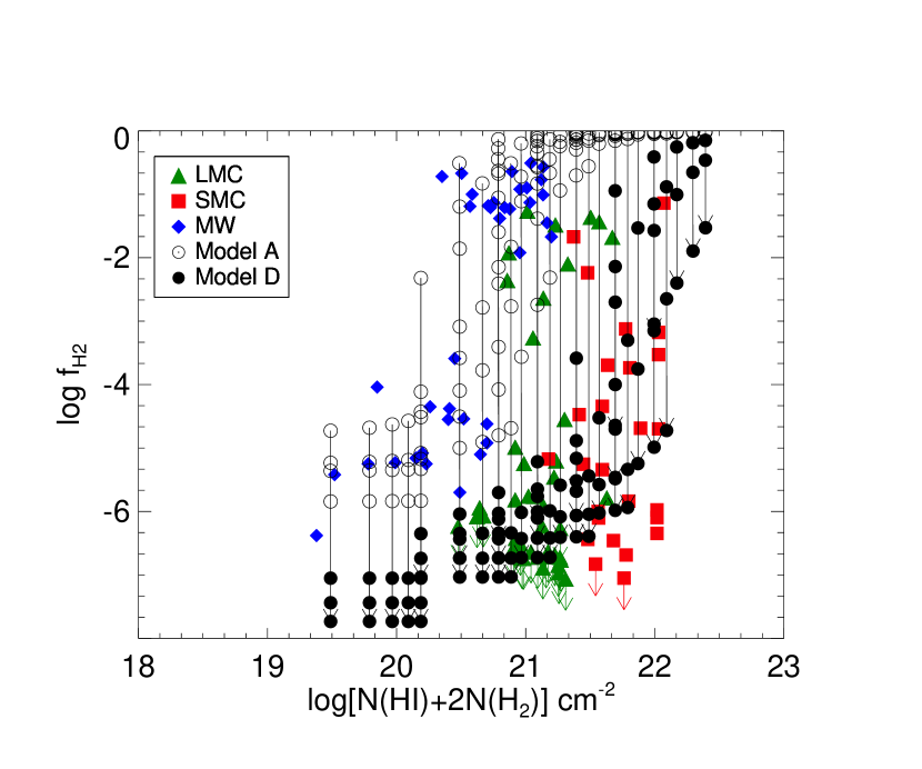
Figure 8: Molecular fractions of SMC, LMC, and Milky Way samples plotted against total H content and compared to model grids. Models in grid A, designated by open circles, have Galactic values of $R$, $I$, and the full range of kinetic temperature, gas density, and cloud size. Models in grid D, designated by filled circles, have the same range of temperature, density, and size, but have $R=3\times 10^{-18}$ cm³ s^-1, $\sim$ 0.1 times the Galactic rate, and $I=10-100$ times the $\sim$ Galactic value. Also shown are lines connecting points in grid A to the correspoding points in grid D; connected points have all properties except radiation field and grain formation rate in common. The agreement with the LMC and SMC data indicates enhanced radiation and reduced grain formation rate of H₂ in the Clouds. See text for more discussion.

In Figure 8, we compare the observed molecular fractions from the LMC, SMC, and Milky Way samples, with our model clouds. Model grid A, representing typical Galactic conditions, and model grid D, which has both an enhanced radiation field ($I=10^{-7}-10^{-6}$ photons cm^-2 s^-1 Hz^-1) and reduced grain formation rate coefficient ($R=3\times 10^{-18}$ cm³ s^-1), are overlaid with the data. Also shown are lines connecting points in grids A and D with the same density, size, and temperature, but different radiation fields and grain formation rates. These lines illustrate the general trend, noted above, that enhancing the radiation field and/or lowering the grain formation rate tends to lower the molecular fraction as well as shift the characteristic breakpoint in column density between gas that is strongly self-shielding and gas that is not.

While the models in grid A match the Galactic points (in blue) fairly well, they do not overlap with the LMC or SMC points at all. Model grids which have either the enhanced radiation field or reduced grain formation rate of grid D, but not both, are also generally overabundant in H₂ relative to the data; these intermediate grids are not shown here. Only the extreme case of model D is able to match the abundance pattern of most of the LMC and SMC points.

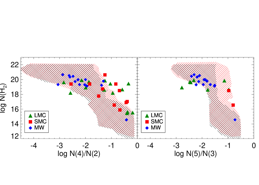
Figure 9: Total column density of H₂ versus excitation ratios N(4)/N(2) and N(5)/N(3), for LMC, SMC, and Galactic data points. The region shaded in both black and red includes all points on this plot which are covered by single cloud models. The region shaded only in red indicates the area covered by concatenations of any two clouds from the model grids. Such concatenations may explain LMC/SMC points that cannot be reached by single-cloud models. See §6 for discussion.

In Figure 9, we examine the column density ratios, N(4)/N(2) and N(5)/N(3), of the three samples, together with shaded regions indicating model points and two-cloud concatenations. The difference between the excitation patterns observed in the LMC or SMC and that in the Milky Way is readily apparent. To try to explain it, we turn to the same grids of models used in analyzing the molecular fraction data. Again, grids representing typical Galactic conditions cannot duplicate the observed excitation pattern – see Tumlinson et al. (2002) for a comparison of individual model grids with the data. The best match to the data is achieved by models with both low $R$ and high $I$.

There are still some LMC and SMC points whose excitation ratios cannot be explained, even by models with enhanced $I$ and reduced $R$. These points may be concatenations of multiple clouds, as described above, although to explain some of the N(4)/N(2) observations, one of the component clouds must be quite hot ($T>$ 400 K). We note that such hot clouds of H₂ may not be possible, since H₂ formation may be strongly suppressed at temperatures $T\gtrsim 200$ K (Shull & Beckwith 1982). In Figure 9, the region shaded red and black indicates the area of the excitation plots that can be reached by single-model clouds in grid D, discussed above; the region covered only by red lines indicates points in the excitation plot that can only be reached by a concatenation of two model clouds. Much of the data can be matched by such concatenations, but some observed N(4)/N(2) ratios are still unexplained. The highest N(5)/N(3) ratios are achieved by combinations in which one cloud is exposed to a relatively low radiation field (roughly Galactic mean intensity), and another is exposed to a very high radiation field (10 to 100 times Galactic mean). This is unsurprising, since the highest N(5)/N(3) ratios are achieved by combinations of clouds with the lowest population in $J=3$ (low radiation field) and clouds with the highest population in $J=5$ (high radiation field). Because a concatenation of multiple clouds can duplicate an overall increase in radiation field intensity, if all the lines of sight studied here are actually composed of multiple components, the very high radiation field suggested here would be unnecessary. However, it seems unlikely that such concatenations would occur much more often in the Clouds than in the Milky Way and thus explain all the observed populations.

A number of potential alternative processes do not suffice to explain the observed LMC/SMC properties:

• The disparity between the LMC/SMC points and the Galactic ones cannot be due solely to differing kinetic temperatures in the two environments. In the model grid with Galactic conditions, the coldest clouds (with $T=10$ K) show the highest N(4)/N(2) and N(5)/N(3) ratios. Decreasing the kinetic temperature below this point is physically unreasonable and has only a marginal effect; increasing it only moves the model points farther away from the LMC/SMC data.

• “Formation pumping,” the idea that H₂ formation may preferentially populate high-J levels, does not suffice to explain the observed excitation. Because absorption in the Lyman and Werner bands is followed by photodissociation only $\sim$ 11% of the time, and because formation must balance photodissociation rather than total absorption, the formation distribution of molecules has a small effect on the final column densities. We have run sample calculations in which all formation was into the $J=4$ and $J=5$ levels, yet even in this extreme case the resulting level populations are not appreciably different from those given here.

We conclude, on the basis of the abundance and excitation data presented above, that H₂ in the SMC and LMC is formed on grains at a rate approximately 10-40 % that in the Galaxy, and that some of the H₂ is exposed to a radiation field 10-100 times more intense than the Galactic one. Ensembles of models under those conditions, though not unique, can reproduce the observed abundance and excitation patterns. There is some evidence that some of the LMC/SMC gas is exposed to a weaker (roughly Galactic) radiation field; not all of the observed sightlines display high H₂ rotational excitation, and as noted above, the best matches to the highest observed ratios come from combinations of clouds where one component is irradiated by a very strong field and the other is exposed to a weaker field. There is probably a blend of environments for H₂ in the Clouds, whereby some of the gas is irradiated at levels not much more intense than in the Milky Way. However, a portion of the H₂ must be exposed to the very high radiation fields noted here in order to explain the observed excitations and molecular fractions.

The above ideas are qualitatively in keeping with the low dust-to-gas ratios previously deduced for the Magellanic Clouds (Koornneef 1982; Fitzpatrick 1985). Those ratios imply a smaller grain surface area per H atom (hence lower $R$) and less attenuation of incident radiation.

7 Conclusions

We have presented computational models of clouds of H₂ and selected applications of those models to FUSE observations. Relatively simple models can duplicate the observed properties of diffuse and translucent clouds fairly well, but there are complications.

Changes in the major physical parameters of such clouds can have many competing effects on observables, and we have demonstrated the general trends obeyed by changes in each parameter. The effects of changes in one parameter can be mirrored by changes in others, so uniquely identifying a line of sight with one set of physical properties is in some cases not feasible. Rather, consideration should be given to the classes of models which can fit a given ensemble of observations.

We suggest that some high-$N(H_{2})$ “clouds” may be separate and physically distinct absorbers viewed along a common line of sight. This interpretation is supported by the fact that the modeled rotational excitation matches the observations, but also by what is needed if one does not allow such combinations: the high-$N(H_{2})$ cloud targets can generally be matched by a single cloud only if that cloud is exposed to a high ($\gtrsim$ 20 times Galactic mean) radiation field. For some Galactic targets, such a radiation field is probably not likely; to explain these observations without recourse to high radiation field requires some additional pathway by which radiation may enter the system. Multiple-component clouds represent such a pathway, if each cloud is physically distinct from the others and therefore does not filter out the incident radiation.

Finally, we have illustrated the application of the code to a large FUSE survey of H₂ in the LMC and SMC. Ensembles of models, though not unique, can match the observed patterns of molecular abundance and rotational excitation. We find evidence for an enhanced UV radiation field (10 to 100 times the Galactic mean), and a reduced grain formation rate of H₂ ($R\approx 3\times 10^{-18}$ cm³ s^-1, one-tenth the nominal Galactic rate).

Table 1: Reference cloud  model column densities (cm^-2)

Level	C1	vDB C1	C4	vDB C4	C7	vDB C7	C10	vDB C10
$J=0$	3.9$\times 10^{20}$	4.1$\times 10^{20}$	3.5$\times 10^{20}$	3.7$\times 10^{20}$	2.5$\times 10^{20}$	2.7$\times 10^{20}$	1.5$\times 10^{20}$	1.6$\times 10^{20}$
$J=1$	1.3$\times 10^{18}$	5.5$\times 10^{18}$	4.5$\times 10^{19}$	5.0$\times 10^{19}$	1.3$\times 10^{20}$	1.5$\times 10^{20}$	2.4$\times 10^{20}$	2.6$\times 10^{20}$
$J=2$	2.0$\times 10^{17}$	1.9$\times 10^{17}$	2.1$\times 10^{17}$	1.8$\times 10^{17}$	1.5$\times 10^{17}$	3.1$\times 10^{17}$	6.7$\times 10^{17}$	2.8$\times 10^{17}$
$J=3$	3.5$\times 10^{15}$	4.3$\times 10^{15}$	5.8$\times 10^{15}$	3.9$\times 10^{15}$	8.4$\times 10^{15}$	1.4$\times 10^{16}$	1.2$\times 10^{16}$	3.5$\times 10^{16}$
$J=4$	1.5$\times 10^{15}$	1.4$\times 10^{15}$	1.5$\times 10^{15}$	1.4$\times 10^{15}$	1.1$\times 10^{15}$	1.3$\times 10^{15}$	8.8$\times 10^{14}$	1.2$\times 10^{15}$
$J=5$	8.3$\times 10^{13}$	7.5$\times 10^{13}$	1.2$\times 10^{14}$	1.4$\times 10^{14}$	1.5$\times 10^{14}$	2.1$\times 10^{14}$	1.9$\times 10^{14}$	2.8$\times 10^{14}$
$J=6$	3.8$\times 10^{13}$	2.9$\times 10^{13}$	3.5$\times 10^{13}$	2.9$\times 10^{13}$	3.0$\times 10^{13}$	2.6$\times 10^{13}$	2.7$\times 10^{13}$	2.5$\times 10^{13}$

Note. — Models with prefix “vDB” are from van Dishoeck & Black (1987), and are labeled as in that text. Models without a prefix are comparable to the corresponding model from vDB.

Table 2: One and two-sided slab models

Label	N(0)	N(1)	N(2)	N(3)	N(4)	N(5)	N(6)
	(cm-2)	(cm-2)	(cm-2)	(cm-2)	(cm-2)	(cm-2)	(cm-2)
One-sided	2.8$\times 10^{20}$	8.1$\times 10^{18}$	5.2$\times 10^{18}$	7.9$\times 10^{16}$	1.3$\times 10^{15}$	3.4$\times 10^{14}$	4.3$\times 10^{13}$
Two-sided	2.7$\times 10^{20}$	8.1$\times 10^{20}$	5.9$\times 10^{18}$	8.8$\times 10^{16}$	1.4$\times 10^{15}$	3.7$\times 10^{14}$	4.6$\times 10^{13}$

Table 3: Column densities for models  exposed to flat and variable radiation fields

Spectrum	N(0)	N(1)	N(2)	N(3)	N(4)	N(5)	N(6)
	(cm-2)	(cm-2)	(cm-2)	(cm-2)	(cm-2)	(cm-2)	(cm-2)
Flat	3.9$\times 10^{20}$	1.3$\times 10^{18}$	2.0$\times 10^{17}$	3.5$\times 10^{15}$	1.5$\times 10^{15}$	8.3$\times 10^{13}$	3.8$\times 10^{13}$
Draine78	3.4$\times 10^{20}$	1.3$\times 10^{17}$	2.5$\times 10^{17}$	5.0$\times 10^{15}$	2.0$\times 10^{15}$	1.2$\times 10^{14}$	5.4$\times 10^{13}$

Table 4: H₂ Cloud Model Grid

Label	R $(10^{-17})$	$I(10^{-8})$	Description
	(cm3 s-1)	(ph cm-2 s-1 Hz-1)
A	1 - 3	1 - 4	Galactic conditions
B	0.3	1 - 4
C	1 - 3	10 - 100
D	0.3	10 - 100	LMC, SMC

Figure 1: FUSE observations of the (4-0) Lyman band for five sightlines in different $N(H_{2})$ regimes. Note the effects of line overlap of the R(0), R(1), and P(1) lines (1049–1051 Å) as $N(H_{2})$ approaches 10²¹ cm^-2.

Figure 2: Simulated spectra near the (4-0) Lyman band for a cloud of physical density $n_{H}=70$ cm^-3 and temperature T = 98 K. Dashed-dot line corresponds to $N(H_{2})$ = $1.2\times 10^{20}$ cm^-2; solid line corresponds to $1.2\times 10^{16}$ cm^-2.

Figure 3: Model clouds at $I=5\times 10^{-7}$ photons cm^-2 s^-1 Hz^-1, but two different temperatures. Lines are drawn between points for which all properties except temperature are identical. Points shown as diamonds have $T=90$ K, while those shown as triangles are at $T=10$ K. At low column densities, changing the temperature has little effect because collisional effects are unimportant relative to radiative decay. The behavior at higher $N(H_{2})$ is set by whether collisions are important in populating $J=1$ and $J=2$. See text for discussion.

Figure 4: Molecular fraction versus total hydrogen column density, and column density of H₂ versus rotational excitation ratio in $J=4$ and $J=2$. The left panels show model clouds exposed to Galactic mean UV radiation field, together with models exposed to a field 50 times more intense. The right panels show models at Galactic radiation field and grain formation rate coefficient $R$, together with models with a grain formation rate one-tenth the Galactic value. Enhancing the radiation field or decreasing the grain formation rate lowers the total abundance of H₂ and pushes the transition to high molecular fraction towards higher column densities. It also raises the excitation ratio N(4)/N(2). The change in excitation is more pronounced for changes in the radiation field than for changes to the grain formation rate.

Figure 5: Comparison of scaling relation for molecular fraction (see §3.6) with models. Models shown in far left panel have a range of densities, but with grain formation rate and UV radiation field equal to the nominal Galactic values. Agreement between the models and the scaling relation is quite good under these conditions. Models in the middle panel have a range of densities, with UV radiation field equal to the nominal Galactic value and grain formation rate $R$ varying from $3\times 10^{-18}$ to $3\times 10^{-17}$ cm³ s^-1. Agreement between the models and the scaling relation is fairly good, particularly at higher molecular fractions. Models in the rightmost panel have a UV radiation field in the range $I=(1-10)\times 10^{-8}$ photons cm^-2 s^-1 Hz^-1 and grain formation rate $R$ varying from $3\times 10^{-18}$ to $3\times 10^{-17}$ cm³ s^-1. Agreement between the models and the scaling relation is fairly good at high molecular fractions but poor at the lowest ones, corresponding to $I$ in excess of about $8\times 10^{-8}$ photons cm^-2 s^-1 Hz^-1.

Figure 7: Column density $N(H_{2})$ in cm^-2 vs. ratio, N(4)/N(2), in rotational states $J=4$ and $J=2$. Models exposed to a high radiation field (10^-7 phot cm^-2 s^-1 Hz^-1, $\sim$ 10 times Galactic) but of varying density and size, together with a region corresponding to the measurement and error bars associated with measurement of H₂ towards AV 47 (designated by the bars). Models shown as diamonds are at 120 K, models shown as circles are at 10 K. Multiple models from these two disparate temperature regimes fall within the region permitted by the error bars.

References

- (1) Abgrall, H., et al. 1994, Can J. Phys, 72, 856
- (2) Black, J. H., & Dalgarno, A. 1973, ApJ, 184, L101
- (3) Black, J. H., & Dalgarno, A. 1976, ApJ, 203, 132
- (4) Black, J. H., & Dalgarno, A. 1977, ApJS, 34, 405
- (5) Black, J. H., & van Dishoeck, E. 1987, ApJ, 322, 412
- (6) Boulanger, F., et al. 2000, in Molecular Hydrogen in Space, ed. F. Combes, & G. Pineau des Forets (Cambridge: Cambridge University Press)
- (7) Carruthers, G. R. 1967, ApJ, 148, L141
- (8) Dalgarno, A., Black, J. H., & Weisheit, J. C. 1973, Ap. Letters, 14, 77
- (9) Draine, B. T., Bertoldi, F. 1996, ApJ, 468, 269
- (10) Draine, B. T. 1978, ApJS, 36, 595.
- (11) Ferlet, R., et al. 2000, ApJ, 538, L69
- (12) Fitzpatrick, E. L. 1985, ApJS, 59, 77
- (13) Gerlich, D. 1990, JChPh, 92, 2377
- (14) Gry, C., et al. 2002, A&A, 391, 675
- (15) Herbst, E. 2000, in Molecular Hydrogen in Space, ed. F. Combes, & G. Pineau des Forets (Cambridge: Cambridge University Press)
- (16) Hollenbach, D., Werner, M., & Salpeter, E. 1971, ApJ, 163, 165
- (17) Jura, M. 1974 ApJ, 191, 375
- (18) Jura, M. 1975a ApJ, 197, 575
- (19) Jura, M. 1975b ApJ, 197, 581
- (20) Katz, N., et al. 1999, ApJ, 522, 305
- (21) Koornneef, J. 1982, A&A, 107, 247
- (22) Le Bourlot, J., et al. 1999, MNRAS, 305, 802
- (23) Moos, H. W., et al. 2000, ApJ, 538, L1
- (24) Rachford, B., et al. 2001, ApJ, 555, 839
- (25) Roberge, W., et al. 1981, ApJ, 243, 817
- (26) Sahnow, D., et al. 2000, ApJ, 538, L7
- (27) Shull, J. M. 1978, ApJ, 219, 877
- (28) Shull, J. M., & Beckwith, S. 1982, ARA&A, 20, 163
- (29) Shull, J. M., et al. 2000, ApJ, 538, L73
- (30) Snow, T. P., et al. 2000, ApJ, 538, L65
- (31) Snow, T. P. 2000, in Molecular Hydrogen in Space, ed. F. Combes, & G. Pineau des Forets (Cambridge: Cambridge University Press)
- (32) Spitzer, L., & Zweibel, E. G. 1974, ApJ, 191, L127
- (33) Sternberg, A. 1988, ApJ, 332, 400
- (34) Sternberg, A., & Dalgarno, A. 1989, ApJ, 338, 197
- (35) Tumlinson, J., et al. 2002, ApJ in press
- (36) van Dishoeck, E., & Black, J. H. 1986, ApJS, 62, 109 (vDB)
- (37) Wolfire, M. G., Hollenbach, D., McKee, C. F., Tielens, A. G. G. M., & Bakes, E. L. O. 1995, ApJ, 443, 152
- (38) Wolniewicz, L., Simbotin, I., & Dalgarno, A. 1998, ApJS, 115, 293