Detecting Topology in a Nearly Flat Spherical Universe

Abstract

When the density parameter is close to unity, the universe has a large curvature radius independently of its being hyperbolic, flat, or spherical. Whatever the curvature, the universe may have either a simply connected or a multiply connected topology. In the flat case, the topology scale is arbitrary, and there is no a priori reason for this scale to be of the same order as the size of the observable universe. In the hyperbolic case any nontrivial topology would almost surely be on a length scale too large to detect. In the spherical case, by contrast, the topology could easily occur on a detectable scale. The present paper shows how, in the spherical case, the assumption of a nearly flat universe simplifies the algorithms for detecting a multiply connected topology, but also reduces the amount of topology that can be seen. This is of primary importance for the upcoming cosmic microwave background data analysis.

This article shows that for spherical spaces one may restrict the search to diametrically opposite pairs of circles in the circles-in-the-sky method and still detect the cyclic factor in the standard factorization of the holonomy group. This vastly decreases the algorithm’s run time. If the search is widened to include pairs of candidate circles whose centers are almost opposite and whose relative twist varies slightly, then the cyclic factor along with a cyclic subgroup of the general factor may also be detected. Unfortunately the full holonomy group is, in general, unobservable in a nearly flat spherical universe, and so a full 6-parameter search is unnecessary. Crystallographic methods could also potentially detect the cyclic factor and a cyclic subgroup of the general factor, but nothing else.

1 Introduction

Recent cosmic microwave background (CMB) data analysis suggests an approximately flat universe. The constraint on the total density parameter, $\Omega$, obtained from CMB experiments depends on the priors used during the data analysis. For example with a prior on the Hubble parameter and on the age of the universe, recent analysis [1, 2] of the DASI, BOOMERanG, MAXIMA and DMR data lead to $\Omega=0.99\pm 0.12$ at 1$\sigma$ level and to $\Omega=1.04\pm 0.05$ at 1$\sigma$ level if one takes into account only the DASI, BOOMERanG and CBI data. Including stronger priors can indeed sharpen the bound. For instance, including information respectively on large scale structure and on supernovae data leads to $\Omega=1.01_{-0.06}^{+0.09}$ and $\Omega=1.02_{-0.08}^{+0.09}$ at 1$\sigma$ level while including both finally leads to $\Omega=1.00_{-0.06}^{+0.10}$. In conclusion, it is fair to retain that current cosmological observations only set the bound $0.9<\Omega<1.1$. These results are consistent with Friedmann-Lemaître universe models with spherical, flat or hyperbolic spatial sections. In the spherical and hyperbolic cases, $\Omega\approx 1$ implies that the curvature radius must be larger than the horizon radius. In all three cases – spherical, flat, and hyperbolic – the universe may be simply connected or multiply connected, but our chances of detecting the topology observationally depend strongly on the curvature.

The chances of detecting a multiply connected topology are worst in a large hyperbolic universe. The reason is that the typical translation distance between a cosmic source and its nearest topological image seems to be on the order of the curvature radius, but when $\Omega\approx 1$ the horizon radius is less than half that distance. For example, if $\Omega_{m}=0.34$, $\Omega_{\Lambda}=0.64$ and $\Omega=0.98$, then the radius $\chi_{\rm LSS}$ of the last scattering surface is 0.43 radians (see Eq. 7 below). As $\Omega$ approaches 1, $\chi_{\rm LSS}$ approaches 0 radians, which is much less than the typical topology scale, making the topology undetectable (see e.g. Refs [3, 4, 5] for some studies on detectability of nearly flat hyperbolic universes). Note that, in spite of a widespread myth to the contrary, the topology scale in a hyperbolic 3-manifold might not depend on the manifold’s volume. It might remain comparable to the curvature radius even for large manifolds, assuming the observer sits at a generic point in the manifold. On the other hand, in the exceptional case that the observer sits near a short closed geodesic, his or her nearest translated image may be arbitrarily close, even in an arbitrarily large manifold.

In a multiply connected flat universe the topology scale is completely independent of the horizon radius, because Euclidean geometry – unlike spherical and hyperbolic geometry – has no preferred scale and admits similarities. A great deal of luck would be required for the topology scale to be less than the horizon radius but still large enough to accommodate the lack of obvious local periodicity. Detecting such a topological structure would naturally raise deep questions about this “topological” coincidence: why is the topology scale of the order of the size of the observable universe today?

In a spherical universe the topology scale depends on the curvature radius, as in the hyperbolic case. Luckily, in contrast to the hyperbolic case, as the topology of a spherical manifold gets more complicated, the typical distance between two images of a single cosmic source decreases. No matter how close $\Omega$ is to 1, only a finite number of spherical topologies are excluded from detection. For example, if $\Omega_{m}=0.34$, $\Omega_{\Lambda}=0.68$ and $\Omega=1.02$, then $\chi_{\rm LSS}$ = 0.43 radians, and the only excluded topologies are those for which the cyclic factor (see Section 2 for explanations) has order at most ${2\pi}/({2\chi_{LSS}})\approx 7$. As $\Omega$ gets closer to 1, more topologies are excluded from observation; nevertheless the chances of observing a spherical universe remain vastly better than the chances of observing a flat universe, because in the flat case only a finite range of length scales are short enough to be observable while an infinite range is too large. The particular case of the detectability of lens spaces was studied in Ref. [9] (which also considers the detectability of hyperbolic topologies).

The present paper investigates how the assumption of a nearly flat ($\Omega\approx 1)$ spherical universe affects the strategy for detecting its topology (see Refs. [10, 11, 12] for reviews on the different methods and their observational status). We find that the circles-in-the-sky method [13] typically detects only a cyclic subgroup of the holonomy group, so the universe “looks like a lens space” no matter what its true topology is. If it looks like a globally homogeneous lens space (generated by a Clifford translation – to be defined in Section 3), then the circles-in-the-sky search reduces from a 6-parameter search space to a 3-parameter space (if the radius $\chi_{\rm LSS}$ of the last scattering surface is known) or a 4-parameter space (if $\chi_{\rm LSS}$ is unknown). Assuming each parameter is tested at $\sim 10^{3}$ points, the total run time decreases by a factor of $\sim 10^{9}$ or $\sim 10^{6}$. If the universe looks like a non globally homogeneous lens space, meaning that a larger subgroup of the holonomy group is detectable, generated by a pair of Clifford translations, then the matching circles lie in a 6-parameter space, but with strong constraints on their values, so the search is still much faster than in the general case.

We also note that the crystallographic method’s pair separation histogram [14] is well suited to detect a topological signal in a nearly flat spherical universe because of the abundance of Clifford translations (defined below).

Section 2 reviews the classification of spherical 3-manifolds. Section 3 defines Clifford translations and explains their cosmological significance. Section 4 analyzes the circles-in-the-sky method, and Section 5 analyzes the crystallographic methods.

2 Classification of Spherical 3-Manifolds

Spherical 3-manifolds were originally classified by Threlfall and Seifert [15] in 1930. Gausmann et al. [16] reformulates Threlfall and Seifert’s classification in terms of single action, double action, and linked action manifolds. This latter work also describes the manifolds in each category, and investigates the topological signature of each in the pair separation histogram of cosmic crystallography.

Interactive software for visualizing these manifolds may be downloaded at www.northnet.org/weeks/CurvedSpaces. The user flies around in spherical 3-manifolds to gain intuition about their topological properties. For instance, the role of a cyclic factor (as described below) can be well understood with this tool; screenshots appear in Figs. (5-7).

In this section, we briefly review the classification given as given in Ref. [16]. Even though we could follow Threlfall and Seifert’s purely geometric approach, i.e. working with right- and left-handed screw motions, we instead borrow from Thurston’s approach [17] and use quaternions to streamline the exposition.

Recall that quaternions are like complex numbers, except that while the complex numbers are spanned by two elements 1 and i  satisfying ${\bf i}^{2}=-1$, the quaternions are spanned by four elements elements 1, i, j, and k  satisfying the (non-commutative) multiplication rules

$${\bf i}^{2}={\bf j}^{2}={\bf k}^{2}=-1$$

$${\bf i}{\bf j}=-{\bf j}{\bf i}={\bf k}$$

$${\bf j}{\bf k}=-{\bf k}{\bf j}={\bf i}$$

$${\bf k}{\bf i}=-{\bf i}{\bf k}={\bf j}$$ (1)

A quaternion ${\bf q}=a{\bf 1}+b{\bf i}+c{\bf j}+d{\bf k}$, with $a,b,c,d$ being real numbers, has length $|{\bf q}|=\sqrt{a^{2}+b^{2}+c^{2}+d^{2}}$. The set of unit length quaternions defines the Lie group ${\cal S}^{3}$, combining the geometry of the 3-sphere $S^{3}$ with the multiplicative action of the quaternions, just as the set of unit length complex numbers defines the Lie group ${\cal S}^{1}$, combining the geometry of the circle $S^{1}$ with the multiplicative action of the complex numbers.

2.1 Single action manifolds

Each quaternion, ${\bf q}\in{\cal S}^{3}$, defines one isometry, $\ell_{\bf q}:{\cal S}^{3}\rightarrow{\cal S}^{3}$, by left multiplication $\ell_{\bf q}({\bf x})={\bf q}{\bf x}$

$$\ell_{\bf q}:\left\{\begin{array}[]{l}{\cal S}^{3}\rightarrow{\cal S}^{3}\\ {\bf x}\mapsto\ell_{\bf q}({\bf x})={\bf q}{\bf x}.\end{array}\right.$$ (2)

Another isometry, $r_{\bf q}:{\cal S}^{3}\rightarrow{\cal S}^{3}$, can analogously be defined by right multiplication $r_{\bf q}({\bf x})={\bf x}{\bf q}$. If $G$ is a finite subgroup of ${\cal S}^{3}$, then $\Gamma=\{\ell_{\bf q}\,|\,{\bf q}\in G\}$ is a finite group of isometries of $S^{3}$ (and isomorphic to ${\cal S}^{3}$). Except for the identity, the isometries in $\Gamma$ have no fixed points, so that $\Gamma$ defines the holonomy group of a spherical 3-manifold. The manifolds that arise in this way are called single action spherical 3-manifolds. Had we used $r_{\bf q}$ instead of $\ell_{\bf q}$ in the definition of $\Gamma$ we would have obtained the mirror image of the same manifold.

The single action manifolds are in one-to-one correspondence with the finite subgroups of ${\cal S}^{3}$, listed in Table 1. Section 3 of Ref. [16] explains the relationship between these subgroups of Isom($S^{3}$) and the corresponding subgroups of Isom($S^{2}$), while Appendix B of Ref. [16] explicitly determines the elements in each group both as quaternions and as $SO(4)$-matrices.

Name of the manifold	Symbol	Order	Fundamental domain
cyclic	$Z_{n}$	$n$	lens
binary dihedral	$D^{*}_{m}$	$4m$	$2m$-sided prism
binary tetrahedral	$T^{*}$	24	octahedron
binary octahedral	$O^{*}$	48	truncated cube
binary icosahedral	$I^{*}$	120	dodecahedron

Table 1: Finite subgroups of ${\cal S}^{3}$. There is a two-to-one homomorphism from ${\cal S}^{3}$ to $SO(3)$ (see Ref. [16] for details) so the finite subgroups of $SO(3)$ – the cyclic, dihedral, tetrahedral, octahedral and icosahedral groups – lift to ${\cal S}^{3}$. Each such group lifts two-to-one, giving the corresponding binary group. Only the cyclic groups of odd order lift one-to-one. That is, each even-order cyclic group $Z_{2n}\subset{\cal S}^{3}$ arises as the two-fold cover of $Z_{n}\subset SO(3)$, while each odd-order cyclic group $Z_{n}\subset{\cal S}^{3}$ is the one-to-one lift of $Z_{n}\subset SO(3)$. The binary polyhedral groups are not merely the product of the original polyhedral groups with a $Z_{2}$ factor, nor are they isomorphic to the so-called extended polyhedral groups containing orientation-reversing as well as orientation-preserving isometries; rather they are something completely new. The plain dihedral, tetrahedral, octahedral and icosahedral groups do not occur as subgroups of ${\cal S}^{3}$.

2.2 Double action manifolds

In a double action spherical 3-manifold two groups act simultaneously, one by left multiplication and the other by right multiplication. That is, each pair of quaternions $({\bf q},{\bf q}^{\prime})\in G\times G^{\prime}\subset{\cal S}^{3}\times{\cal S}^{3}$ defines an isometry by simultaneous left and right multiplication

$$d_{{\bf q},{\bf q}^{\prime}}:\left\{\begin{array}[]{l}{\cal S}^{3}\rightarrow{\cal S}^{3}\\ {\bf x}\mapsto d_{{\bf q},{\bf q}^{\prime}}({\bf x})={\bf q}{\bf x}{\bf q}^{\prime}.\end{array}\right.$$ (3)

The resulting group $\Gamma=\{d_{{\bf q},{\bf q}^{\prime}}\,|\,({\bf q},{\bf q}^{\prime})\in G\times G^{\prime}\}$ will be fixed point free (and thus define a manifold) if and only if the orders of $G$ and $G^{\prime}$ are relatively prime, with the possible exception of a common factor of two corresponding to the quaternion $-{\bf 1}$. The binary polyhedral groups all contain elements of order 4 (see Table 1) and therefore cannot be paired with each other. Thus either $G$ or $G^{\prime}$ must be cyclic. Without loss of generality we henceforth assume that in a double action manifold the second factor $G^{\prime}$ is cyclic. The first factor $G$ may be either cyclic or binary polyhedral.

2.3 Linked action manifolds

Linked action spherical 3-manifolds are similar to double action manifolds. One begins with a pair of groups $G$ and $G^{\prime}$ whose orders are not relatively prime, but then takes $\Gamma\subset\{d_{{\bf q},{\bf q}^{\prime}}\,|\,({\bf q},{\bf q}^{\prime})\in G\times G^{\prime}\}$ to be a subgroup avoiding elements $d_{{\bf q},{\bf q}^{\prime}}$ with fixed points. The only examples of linked action manifolds are the following:

• $G$ and $G^{\prime}$ are both cyclic and $\Gamma$ is the holonomy group of a lens space $L(p,q)$.

• $G=T^{*}$, $G^{\prime}=Z_{9n}$ ($n$ odd), and $\Gamma$ is a (fixed point free) subgroup of index 3 in the full (fixed point containing) double action group.

• $G=D^{*}_{m}$, $G^{\prime}=Z_{8n}$ ($m$ odd and relatively prime to $n$), and $\Gamma$ is a (fixed point free) subgroup of index 2 in the full (fixed point containing) double action group.

Section 4.3 of Ref. [16] explains these manifolds in greater detail.

3 Clifford Translations

Each left multiplication $\ell_{\bf q}$ defines a Clifford translation because it translates all points the same distance – that is, ${\rm dist}({\bf x},\ell_{\bf q}({\bf x}))$ is constant for all ${\bf x}\in{\cal S}^{3}$ – and similarly for each right multiplication $r_{\bf q}$. Clifford translations play a crucial role in cosmic topology. As will be detailed later, the circles-in-the-sky method [13] works best with them, and the pair separation histogram (PSH) method of cosmic crystallography detects only Clifford translations [18].

Just as a Euclidean translation defines a family of parallel lines in the Euclidean plane (Figure 1), a left multiplication $\ell_{\bf q}$ of ${\cal S}^{3}$ defines a family of Clifford parallels on the 3-sphere (Figure 2). To make this precise, replace the static quaternion ${\bf q}=a{\bf 1}+b{\bf i}+c{\bf j}+d{\bf k}$ with a time-dependent quaternion

$${\bf q}(t)=\cos{2\pi t}\,{\bf 1}+\sin{2\pi t}\frac{b\,{\bf i}+c\,{\bf j}+d\,{\bf k}}{\sqrt{b^{2}+c^{2}+d^{2}}},$$ (4)

to generate a flow on $S^{3}$ carrying each point ${\bf x}\in{\cal S}^{3}$ along the flow line ${\bf x}(t)={\bf q}(t){\bf x}$. The flow lines comprise a family of geodesics (i.e. great circles) called Clifford parallels. The flow is homogeneous in the sense that any Clifford parallel is equivalent to any other. Any two nearby Clifford parallels twist around each other exactly once. This remarkable behavior characterizes the geometry of the 3-sphere, distinguishing it from familiar Euclidean geometry.

Each left multiplication $\ell_{\bf q}$ defines a right handed family of Clifford parallels, in the sense that as you move forward along a given parallel, neighboring parallels twist clockwise. Similarly, each right multiplication $r_{\bf q}$ defines a left handed family of Clifford parallels. Henceforth all discussion of $\ell_{\bf q}$ will apply equally well to $r_{\bf q}$, but with opposite chirality. Note that left multiplication defines right handed Clifford parallels while right multiplication defines left handed Clifford parallels. Strictly speaking, an isometry $\ell_{\bf q}$ takes the 3-sphere and simply places it in its new position. In practice, though, one visualizes $\ell_{\bf q}$ as a continuous motion $\ell_{{\bf q}(t)}$ , sliding the 3-sphere from its original position to its final position along the Clifford parallels. Each point moves along a geodesic while nearby points spiral around it. Because of this visual image, each $\ell_{\bf q}$ (resp. $r_{\bf q}$) is called a right handed (resp. left handed) Clifford translation.

If ${\bf q}\neq\pm{\bf 1}$ there is a unique right handed Clifford translation $\ell_{\bf q}$ (and a unique left handed Clifford translation $r_{\bf q}$) taking ${\bf 1}$ to ${\bf q}$, the corresponding Clifford parallels are well defined, and $\ell_{\bf q}\neq r_{\bf q}$. The quaternion $-{\bf 1}$ is exceptional: both $\ell_{-{\bf 1}}$ and $r_{-{\bf 1}}$ are the antipodal map and correspond to translation half way along any set of Clifford parallels. This degeneracy accounts for an exceptional factor of two that runs throughout the theory of spherical 3-manifolds (see Ref. [16]). The quaternion ${\bf 1}$ is also exceptional in that $\ell_{\bf 1}=r_{\bf 1}={\rm Id}$ and corresponds to the null translation on any set of Clifford parallels, but because ${\bf 1}$ is already the identity quaternion it creates no exceptional cases.

Any set of right handed Clifford parallels has exactly two great circles in common with any set of left handed Clifford parallels (Figure 3). Furthermore the two common circles are maximally far from each other: the distance from any point on one of the common circles to any point on the other is exactly $\pi/2$. In a neighborhood of a common circle, a Clifford translation along the right handed parallels twists clockwise while a Clifford translation along the left handed parallels twists counterclockwise.

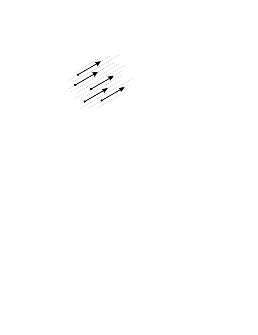
Figure 1: A translation of the Euclidean plane $E^{2}$ (characterized by a vector $\vec{u}$) defines a family of parallel flow lines, in the sense that to any point $M_{0}\in E^{2}$ one can associate the flow $M(t)=M_{0}+t\vec{u}$.

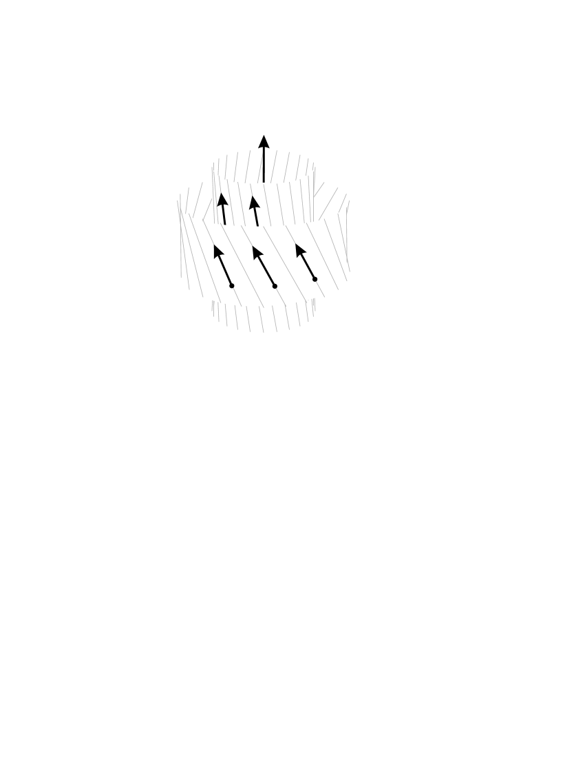
Figure 2: A Clifford translation of the 3-sphere $S^{3}$ defines a family of Clifford parallels. This figure shows a left-handed flow of Clifford parallels (i.e. the flows are spiralling counterclockwise) corresponding to a right multiplication $r_{{\bf q}(t)}$.

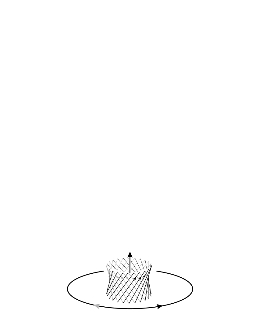
Figure 3: Each set of right handed Clifford parallels (black) has exactly two great circles in common with each set of left handed Clifford parallels (grey). In the neighborhood of one common great circle (central axis) the right handed Clifford parallels twist clockwise while the left handed Clifford parallels twist counterclockwise. In the neighborhood of the other common great circle (equatorial belt) the right and left handed Clifford parallels still twist clockwise and counterclockwise, respectively, but translate in opposite directions.

4 Circle Searching in a Nearly Flat Spherical Universe

The circles-in-the-sky method for detecting cosmic topology relies on the fact that in a sufficiently small universe the last scattering surface will “wrap all the way around the universe” and intersect itself [13] (see also Ref. [12] for a recent review of topology and the CMB). Each circle of self-intersection will appear as two different circles in the sky with matching CMB temperatures (modulo various sources of interference, such as the integrated Sachs-Wolfe effect, the Doppler effect due to the primordial plasma’s motion, and microwave contamination in the plane of the Milky Way). If one can detect matching circles, one can deduce the topology of space [19].

In its most general form, the circles-in-the-sky method searches over a 6-dimensional parameter space: two parameters for the center of the first candidate circle, two parameters for the center of the second candidate circle, one parameter for the circles’ angular radius, and one parameter for the relative twist with which the circles are compared. To test for a nonorientable topology one must, in addition, compare each pair of candidate circles with reversed orientation. A full 6-parameter search is computationally expensive, and simplifications must be found [20].

In this section, we want to show that circle searching is much easier in a nearly flat spherical manifold than in the general case. To fix the notations, the local geometry of the universe is described by a Friedmann–Lemaître metric

$${\rm d}s^{2}=-{\rm d}t^{2}+a^{2}(t)\left({\rm d}\chi^{2}+\sin^{2}{\chi}{\rm d}\omega^{2}\right)$$ (5)

where $a$ is the scale factor, $t$ the cosmic time and ${\rm d}\omega^{2}\equiv{\rm d}\theta^{2}+\sin^{2}{\theta}{\rm d}\varphi^{2}$ the infinitesimal solid angle. $\chi$ is the (dimensionless) comoving radial distance in units of the curvature radius of $S^{3}$, that is, in radians so that $\chi$ runs from 0 to $\pi$. Integrating the radial null geodesic equation ${\rm d}\chi={\rm d}t/a$ leads to

$$\chi(z)=\int_{0}^{z}\frac{\sqrt{\Omega_{m}+\Omega_{\Lambda}-1}\,{\rm d}x}{\sqrt{\Omega_{\Lambda}+(1-\Omega_{m}-\Omega_{\Lambda})(1+x)^{2}+\Omega_{m}(1+x)^{3}}}$$ (6)

where $\Omega_{\Lambda}$ and $\Omega_{m}$ are the cosmological constant and matter density parameters evaluated today. The comoving coordinate of the last scattering surface is thus given by

$$\chi_{\rm LSS}=\chi(z_{\rm LSS})$$ (7)

with $z_{\rm LSS}\sim 1100$.

4.1 Circle searching in a single action manifold

In a single action manifold, every holonomy is a Clifford translation. One visualizes a Clifford translation taking one image of the last scattering surface to another of its images as a translation along a geodesic combined with a simultaneous twist about the same geodesic. Thus every matched circle lies directly opposite its mate. This immediately reduces the parameter space from 6 to 4 dimensions, because the center of one candidate circle completely determines the center of the other. If the universe is nearly flat, the parameter space reduces further: the radius $\chi_{\rm LSS}$ of the last scattering surface (in radians) is small, so any pair of matched circles corresponds to a short translation distance, and hence to a small twist.

Because Clifford translations translate and twist exactly the same amount, the twist angle between two matched circles reveals the translation distance in radians. If the radius $\chi_{\rm LSS}$ of the last scattering surface (in radians) is known (or well estimated) ahead of time, then the matched circles’ angular radius completely determines their twist and vice versa (see Figure 4). This further reduces the search parameter space to 3 dimensions. In other words, the center of one candidate circle determines the center of the other, and their common angular radius determines the twist. Furthermore, the twist is quantized, with values of the form $2\pi/n$ for integer $n$.

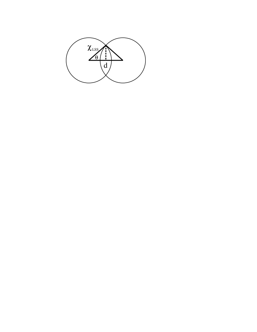
Figure 4: If the radius $\chi_{\rm LSS}$ of the last scattering surface is known in advance (in units of the curvature radius), then the angular diameter $\theta$ of a matched circle determines the distance $d$ to the observer’s translated image (still in curvature units) via spherical trigonometry: $\tan d/2=\tan\chi_{\rm LSS}\cos\theta$. If the translation is a Clifford translation, the twist angle $\varphi$ exactly equals the translation distance $d$.

Group	Min. translation distance	Sample min. $\Omega$
Binary icosahedral $I^{*}$	$2\pi/10$	1.011
Binary octahedral $O^{*}$	$2\pi/8$	1.017
Binary tetrahedral $T^{*}$	$2\pi/6$	1.030
Binary dihedral $D^{*}_{m}$	$2\pi/2m$	$\sim(1+{1}/{(2m)^{2}})$
Cyclic $Z_{n}$	$2\pi/n$	$\sim(1+{1}/{n^{2}})$

Table 2: For each single action manifold, the second column gives the distance from the observer to his or her nearest translated image. The third column tells the minimum value of $\Omega$ required for the last scattering surface to intersect itself. That is, matched circles will occur in the given topology if and only if $\Omega$ exceeds the value given. Strictly speaking, the minimum value of $\Omega$ depends on both $\Omega_{m}$ and $\Omega_{\Lambda}$; for simplicity, the sample values in the third column fix $\Omega_{m}$ at 0.35 and vary $\Omega_{\Lambda}$.

Table 2 shows the distance from a source to its nearest translate in each of the single action manifolds. The table’s third column shows a typical value of $\Omega$ for which the diameter of the last scattering surface drops below the manifold’s minimum translation distance, and the topology becomes undetectable. If the true $\Omega$ exceeds the minimum then nearby images of the last scattering surface overlap and the topology is potentially detectable. The groups $D^{*}_{m}$ and $Z_{n}$ are always detectable for large values of $m$ and $n$, even though low values of $m$ and $n$ may be excluded. The minimum values of $\Omega$ shown in the table were found by using Eq. (7) to compute the radius of the last scattering surface in curvature units as a function of $\Omega_{m}$ and $\Omega_{\Lambda}$. Trial and error quickly revealed which values of $\Omega_{m}$ and $\Omega_{\Lambda}$ were required for the diameter of the last scattering surface to equal the minimum translation distance shown in second column of the table.

4.2 Circle searching in a double action or linked action manifold

Recall from Section 2 that at least one factor in a double action manifold or linked action manifold must be cyclic. Without loss of generality, assume the second factor $G^{\prime}$ is the cyclic group $Z_{n}$. Geometrically, this cyclic factor creates a string of $n$ images of each cosmic source, arranged along a great circle (see Figure 5) and related by left handed Clifford translations. The first factor $G$, which may or may not be cyclic, creates parallel copies of the string of $n$ images (see Figure 5), related by right handed Clifford translations.

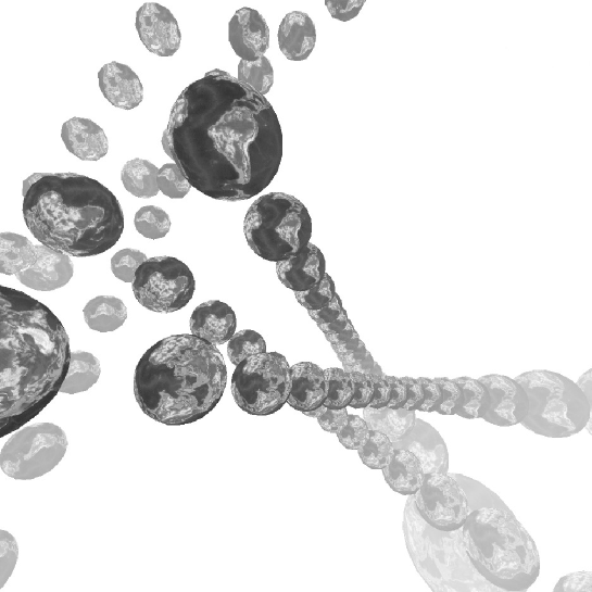
Figure 5: The cyclic factor $G^{\prime}$ generates the images within each string, while the general factor $G$ takes one string to another. A $Z_{3}$ subgroup of $G$ permutes the three nearby strings. The axis of symmetry running along the center of the group of three strings is the common Clifford parallel, belonging to the family of left handed parallels of $G^{\prime}$ as well as the right handed parallels of the $Z_{3}$ subgroup of $G$.

The elements of $G^{\prime}=Z_{n}$ are all powers of a single generator, and therefore translate along the same set of left handed Clifford parallels. The elements of $G$ may make use of several sets of right handed Clifford parallels, one set for each maximal cyclic subgroup of $G$. Each such set of right handed Clifford parallels has exactly two great circles in common with the left handed Clifford parallels of $G^{\prime}$ (recall Section 3 and Figure 3). One such common Clifford parallel lies along the axis of symmetry of the three strings of Earths in Figure 5: it belongs to the set of left handed parallels that translate the Earths within each string, and also belongs to the set of right handed parallels that take one string of Earths to another.

Both sets of Clifford translations preserve the invariant tori centered around the common Clifford parallel (see Figure 3). If both sets of Clifford translations have large order, many images of the observer may crowd the invariant torus (see Figure 6). In the exceptional case that the two sets of Clifford translations have similar order, the closest distance between two images need not be a pure left or right handed Clifford translation, but can be some linear combination of the two.

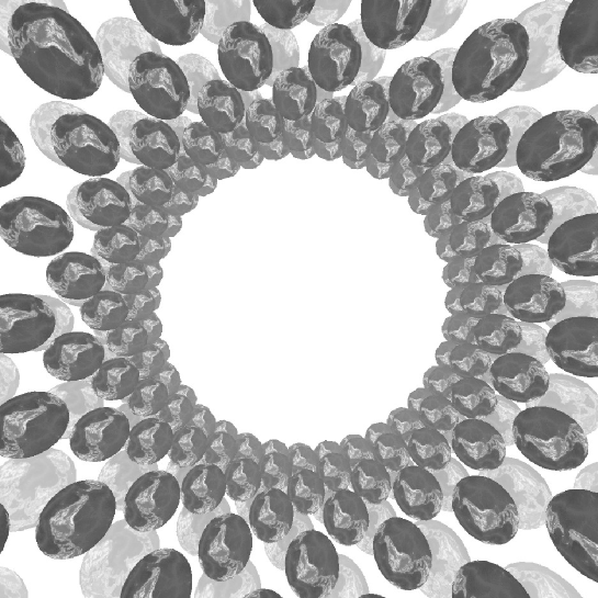
Figure 6: If both $G$ and $G^{\prime}$ are cyclic of large order (here $G\approx Z_{17}$ and $G^{\prime}\approx Z_{19}$), then many images of the observer crowd the invariant torus. The axis of symmetry, orthogonal to the page, is the common Clifford parallel belonging to both $G$ and $G^{\prime}$. Note that the orientation of the images varies smoothly.

Recall that every holonomy of a spherical 3-manifold can be expressed as the composition of a left handed Clifford translation and a right handed Clifford translation (Section 2), and any left handed Clifford translation shares a common axis with any right handed one (see Figure 3). Thus every holonomy of a spherical 3-manifold is a corkscrew motion along the common axis of its left and right handed Clifford factors, and so the situation described above is completely general. Nearby images may depend on only one factor (as in Figure 5) or on both factors (as in Figure 6)

If nearby images depend on only one factor (Figure 5) then only the translates within a single string produce matched circles. Searching for such matched circles is easy: they all come from Clifford translations, so just as in Section 2.1 the center of one matched circle completely determines the center of its mate, and the search space is either 4-dimensional (with no a priori knowledge) or 3-dimensional (if $\chi_{\rm LSS}$ is known in radians). If such circles are found, we detect the cyclic factor $G^{\prime}=Z_{n}$, but remain completely unaware of the other factor $G$. Reversing this logic, if matched circles reveal a cyclic group in the real universe, we cannot automatically conclude that the universe is a lens space, but must consider the possibility of a second factor.

If nearby images depend on both factors (Figure 6) then we must consider the geometry of the invariant torus more carefully. The surface of the invariant torus is locally saddle-shaped. Translations along the left- or right-handed Clifford parallels of Figure 3 are translations along the horizontal lines in Figure 7(left); these translations keep matching circles opposite each other in the sky, but introduce a twist. Pure meridional or longitudinal rotations in Figure 3 are motions in the directions of maximal curvature in Figure 7(right); they displace matching circles so that their centers are no longer exactly opposite, but introduce no twist. Translations in generic directions cause a small displacement of matching circles along with a small twist. The magnitude of the displacement and twist could be large if the Earth happens to lie near the common Clifford parallel, but generically it is small. Thus we must search for circles in a full 6-parameter space, but we may assume that the centers of the matching circles are almost opposite each other and the twist angle is small.

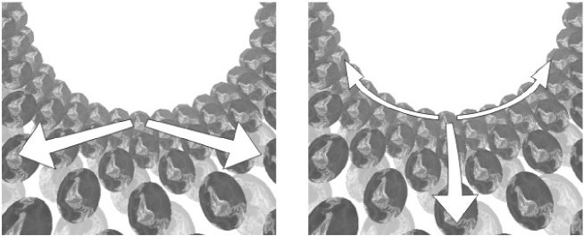
Figure 7: Translations along the Clifford parallels (left) keep matched circles directly opposite their mates while introducing a small twist. Translations in the directions of maximal curvature (right) offset the matched circles’ centers but introduce no twist.

4.3 Matched circles search strategy

The preceding paragraphs tell how to look efficiently for matching circles in a nearly flat spherical universe:

• look for directly opposite circles to detect a single action manifold or a single factor in a double action or linked action manifold (Figure 5)

• or allow small deviations in circle position and twist to detect a more general cyclic subgroup in a double or linked action manifold (Figure 6).

Let us now turn to the question of how much of the topology can be detected using only nearby images of the observer. The cyclic factor $G^{\prime}=Z_{n}$ creates matching circles whenever $\Omega$ is greater than about $1+{1}/{n^{2}}$ (see Table 2). To understand the general factor $G$, think of it as the (non disjoint) union of its maximal cyclic subgroups. Recall that the flow lines of each cyclic subgroup $H\subset G$ share a unique pair of Clifford parallels with the flow lines of $G^{\prime}$ (Figure 3). If the order of $H$ is small, then the parallel strings of images are typically too far apart to create matching circles (Figure 5), and $H$ remains undetectable. (An exceptional case occurs when the observer happens to sit near the common Clifford parallel, in which case the parallel strings of images do get close enough to create matching circles.) If the order of $H$ is large, then parallel strings of images may be close enough to create matching circles (Figure 6). Consulting Table 1, let us consider each possibility for the general factor $G$.

1. If $G$ is the binary tetrahedral group $T^{*}$, the binary octahedral group $O^{*}$, or the binary icosahedral group $I^{*}$, then the largest cyclic subgroup has order 6, 8, or 10, respectively; however such a subgroup contains the antipodal map, so it creates only 3, 4, or 5 strings of images, respectively. If $\chi_{\rm LSS}$ is small (in radians), such parallel strings create no matching circles, and $G$ remains undetectable. In the exceptional case that the Earth lies near a common Clifford parallel, we would detect a single cyclic subgroup of $G$ of order at most 5.

2. If $G$ is a cyclic group $Z_{k}$, it will create matched circles if and only if $k$ is large or the Earth happens to lie near one of the pair of common Clifford parallels that $G$ shares with $G^{\prime}$. In this case all images of the observer lie on a single invariant torus, as shown in Figure 6.

3. If $G$ is a binary dihedral group $D^{*}_{m}$ we get all the images on the invariant torus defined by its cyclic subgroup $Z_{2m}$ as in the previous case (Figure 6), along with a second copy of the invariant torus. Each of the many order 4 elements in $D^{*}_{m}$ interchanges the two invariant tori. In general the two invariant tori are too far apart to create matched circles, so a $D^{*}_{m}\times Z_{n}$ universe would in practice look like a $Z_{2m}\times Z_{n}$ universe. In the exceptional case that the two invariant tori nearly coincide (which occurs only when the observer happens to sit approximately midway between the two common Clifford parallels), an image of the last scattering surface on one invariant torus may intersect an image on the other; it is straightforward to see that the two matching circles would lie in the same part of the sky and overlap each other, but such non-generic behavior is unlikely to be observed in practice. In practice one expects the generic case that matching circles lie approximately (or exactly) opposite one other.

5 Cosmic Crystallography in a Nearly Flat Spherical Universe

The pair separation histogram (PSH) method for detecting cosmic topology [14] relies on the fact that in certain multiply connected topologies, if the comoving distance from one source (for example a galaxy cluster) to its nearest (resp. second nearest, etc.) translated image is $\chi_{\rm gg}$, then the distance from every source to its nearest (resp. second nearest, etc.) translated image is also $\chi_{\rm gg}$. Thus to seek topology, one measures the distances between all pairs of sources (without worrying about which are topological images of one another) and checks whether any distances $\chi_{\rm gg}$ occur extraordinarily often. Crystallographic methods probe topology on the scale of the catalog’s depth $\chi_{\rm catalog}=\chi(z)$ for $z\sim 1-3$, so $\chi_{\rm LSS}$ has to be replaced by $\chi_{\rm catalog}$ in the previous discussion.

Among the hyperbolic topologies, the PSH method never works [18], because the distance from a source to its nearest translated image always depends on the source’s location in the manifold. Among the flat topologies, the PSH method works for the 3-torus, because the distance from a source to its nearest image does not depend on its location, but for all other flat topologies the PSH method detects only a subgroup of the full holonomy group, namely the subgroup of pure translations. Among the spherical topologies, the PSH method detects precisely the Clifford translations (despite all observational uncertainties [21]).

Group	Min. translation distance	Sample min. $\Omega$
Binary icosahedral $I^{*}$	$2\pi/10$	1.048
Binary octahedral $O^{*}$	$2\pi/8$	1.073
Binary tetrahedral $T^{*}$	$2\pi/6$	1.125
Binary dihedral $D^{*}_{m}$	$2\pi/2m$	$\sim(1+{5}/{(2m)^{2}})$
Cyclic $Z_{n}$	$2\pi/n$	$\sim(1+{5}/{n^{2}})$

Table 3: Crystallographic methods probe topology only to a distance of $\chi(z)$ for $z\sim 3$, in which case the minimum values of $\Omega$ given in Table 2 for circle matching at $\chi(z_{\rm LSS})$ must be replaced by the values shown here for crystallographic studies at $\chi(3)$. That is, a $z\leq 3$ catalog may contain repeated images of galaxy clusters in the given topology if and only if $\Omega$ exceeds the value given. As in Table 2 the sample values in the third column fix $\Omega_{m}$ at 0.35 and vary $\Omega_{\Lambda}$.

In a single action manifold (Subsection 2.1) all holonomies are Clifford translations, and thus the topology is potentially detectable if and only if $\Omega$ exceeds the minimum value as illustrated in Table 3. In the case of the binary tetrahedral, binary octahedral, and binary icosahedral groups we would detect equal length translations in several different directions, and could infer the topology exactly. In the case of a binary dihedral group (assuming $\Omega\approx 1$) we would see only the cyclic factor, so in practice we couldn’t distinguish the binary dihedral group from a cyclic group.

In a double action manifold (Subsection 2.2) the PSH could detect the factors $G$ and $G^{\prime}$ individually, subject to the conditions explained in the preceding paragraph, because each is a group of Clifford translations, but it could not detect any nontrivial composite elements $(g,g^{\prime})\in G\times G^{\prime}$. Fortunately our nearest translates will typically be Clifford translates (and thus potentially detectable) even though the vast majority of other translates are not (cf. Figure 5). Only in exceptional cases (namely when $G$ and $G^{\prime}$ are cyclic of comparable order, or the observer is at a non-generic location) might our nearest translates fail to be Clifford translates.

In a linked action manifold (Subsection 2.3) only a subgroup of each factor $G$ and $G^{\prime}$ is available, so it is harder to detect a linked action manifold than a double action one. In some cases, such as the lens space $L(5,2)$, the available subgroups are trivial and the PSH cannot detect the topology at all. Fortunately if one excludes the lens spaces then the remaining linked action manifolds are index 2 or index 3 subgroups of the corresponding double action manifolds, the picture is qualitatively the same as in Figure 5, and again the nearest translates are Clifford translates, which the PSH can detect.

6 Conclusion

In this article, we have studied the detectability of topology when the universe is spherical but nearly flat, both by the CMB-based circle-in-the-sky method and the large scale structure-based crystallographic method.

Spherical topologies turn out to be the most readily detectable. After recalling their geometrical properties, we first showed that the circles-in-the-sky method typically detects only a cyclic subgroup of the holonomy group, so the universe “looks like a lens space” no matter what its true topology is. If it looks like a globally homogeneous lens space, then the circles-in-the-sky search reduces from a 6-parameter search space to a 3-parameter space or a 4-parameter space depending on whether the radius of the last scattering surface is known or not. If the universe looks like a non globally homogeneous lens space then the matching circles lie in a 6-parameter space, but with strong constraints on their values, so that the search is still much faster than in the general case. We also showed that crystallographic methods are well suited to detect the topology of a nearly flat spherical universe thanks to the abundance of Clifford translations.

We hope our analyses and results will serve as preparation for intelligently searching the upcoming MAP satellite data for a topological signal.

References

- [1] J.L. Sievers et al., “Cosmological parameters from Cosmic Background Imager Observations and Comparisons with BOOMERANG, DASI, and MAXIMA3”, [arXiv:astro-ph/0205387].
- [2] C. Netterfield et al., “A measurement by BOOMERANG of angular power spectrum of the cosmic microwave background”, [arXiv:astro-ph/0104460].
- [3] G.I. Gomero, M.J. Reboucas, and R. Tavakol, “Are Small Hyperbolic Universes Observationally Detectable?”, Class. Quant. Grav. 18 (2001) L145, [arXiv:gr-qc/0106044].
- [4] R.Aurich and F.Steiner, “The Cosmic Microwave Background for a Nearly Flat Compact Hyperbolic Universe”, Month. Mot. R. Astron. Soc. 323 (2001) 1016-1024, [arXiv:astro-ph/0007264].
- [5] K.T. Inoue, “Are compact hyperbolic models observationally ruled out?”, Prog. Theor. Phys. 106 (2001) 39, [astro-ph/0102222].
-
[6]
I.Y. Sokolov, JETP Lett. 57 (1993) 617;
A.A. Starobinsky, JETP Lett. 57 (1993) 622;
D. Stevens, D. Scott, and J. Silk, Phys. Rev. Lett. 71 (1993) 20. - [7] K.T. Inoue, “COBE constraints on a compact toroidal low-density universe”, Class. Quant. Grav. 18 (2001) 1967-1977, [arXiv:astro-ph/0011462].
- [8] J. Levin, E. Scannapieco, and J. Silk, “Is The Universe Infinite Or Is It Just Really Big?”, Phys. Rev. D 58 (1998) 103516, [arXiv:astro-ph/9802021].
- [9] G.I. Gomero, M.J. Reboucas, and R. Tavakol, “Detectability of Cosmic Topology in Almost Flat Universes”, Class. Quant. Grav. 18 (2001) 4461-4476, [arXiv:gr-qc/0105002].
- [10] J-P. Uzan, R. Lehoucq, and J-P. Luminet, “New developments in the search for the topology of the universe”, Proc. of the XIXth Texas meeting, Paris 14–18 December 1998, Eds. E. Aubourg, T. Montmerle, J. Paul and P. Peter, article no 04/25, [arXiv:gr-qc/0005128].
- [11] M. Lachièze-Rey and J.-P. Luminet, “Cosmic topology”, Phys. Rept. 254 (1995) 135, [arXiv:gr-qc/9605010].
- [12] J. Levin, “Topology and the cosmic microwave background”, Phys. Rept. 365 (2002) 251, [arXiv:gr-qc/0108043].
- [13] N. Cornish, D. Spergel and G. Starkman, “Circles in the sky: finding topology with the microwave background radiation”, Class. Quant. Grav. 15 (1998) 2657–2670, [arXiv:astro-ph/9801212].
- [14] R. Lehoucq, M. Lachièze-Rey and J.-P. Luminet, “Cosmic crystallography”, Astron. Astrophys. 313 (1996) 339–346, [arXiv:gr-qc/9604050].
- [15] W. Threlfall and H. Seifert, “Topologische Untersuchung der Diskontinuitätsbereiche endlicher Bewegungsgruppen des dreidimensionalen sphärischen Raumes”, Math. Annalen 104 (1930) 1–70 and 107 (1932) 543–586.
- [16] E. Gausmann, R. Lehoucq, J.-P. Luminet, J.-P. Uzan and J. Weeks, “Topological lensing in elliptical spaces”, Class. Quant. Grav. 18 (2001) 5155–5186, [arXiv:gr-qc/0106033].
- [17] W.P. Thurston, Three-dimensional geometry and topology (1997) Princeton Mathematical series 35, Ed. S. Levy, (Princeton University Press, Princeton, USA).
- [18] R. Lehoucq, J-P. Luminet, and J-P. Uzan, Astron. Astrophys. 344 (1999) 735, [arXiv:].
- [19] J. Weeks, “Reconstructing the global topology of the universe from the cosmic microwave background” Class. Quant. Grav. 15 (1998) 2599-2604, [arXiv:astro-ph/9802012].
- [20] N. Cornish, “Implementing the matched circle search with MAP data”, talk at the AMS Special Session on the Geometry and Topology of the Universe, Williams College, Williamstown, US, October 13-14, 2001; [http://www.physics.montana.edu/faculty/cornish/circle_files/v3_document.htm].
- [21] R. Lehoucq, J-P. Uzan, and J-P. Luminet, “Limits of crystallographic methods for detecting space topology”, Astron. Astrophys. 363 (2000) 1, [arXiv:astro-ph/0005515].