Cosmological consequences of a Chaplygin gas dark energy

Abstract

A combination of recent observational results has given rise to what is currently known as the dark energy problem. Although several possible candidates have been extensively discussed in the literature to date the nature of this dark energy component is not well understood at present. In this paper we investigate some cosmological implications of another dark energy candidate: an exotic fluid known as the Chaplygin gas, which is characterized by an equation of state $p=-A/\rho$, where $A$ is a positive constant. By assuming a flat scenario driven by non-relativistic matter plus a Chaplygin gas dark energy we study the influence of such a component on the statistical properties of gravitational lenses. A comparison between the predicted age of the universe and the latest age estimates of globular clusters is also included and the results briefly discussed. In general, we find that the behavior of this class of models may be interpreted as an intermediary case between the standard and $\Lambda$CDM scenarios.

I Introduction

From a large number of observational evidence, the currently favoured cosmological model is flat, accelerated and composed of $\sim 1/3$ of matter (barionic + dark) and $\sim 2/3$ of a negative-pressure dark component, usually named dark energy or “quintessence”. The nature of such an unclustered dark energy component, however, is not very well understood at present, giving rise to many theoretical speculations.

Certainly, the most extensively studied explanation for this dark energy problem is the vaccum energy density or cosmological constant ($\Lambda$) although other interesting possibilities are also alive in the current literature. Some examples are: a very light scalar field $\phi$, whose effective potential $V(\phi)$ leads to an accelerated phase at the late stages of the Universe peebles , a X-matter component turner , which is simply characterized by an equation of state $p_{x}=\omega_{x}\rho_{x}$, where $-1\leq\omega_{x}<0$ and that includes, as a particular case, models with a cosmological constant ($\Lambda$CDM), a vaccum decaying energy density or a time varying $\Lambda$-term whose the present value of the cosmological constant ($\Lambda_{o}$) is a remnant of the primordial inflationary/deflationary stage ozer , geometrical effects from extra dimensions dvali or still an exotic fluid, the so-called Chaplygin gas, whose equation of state is given by

$$p=-A/\rho,$$ (1)

where $A$ is a positive constant kamen .

All the above mentioned candidates for quintessence have interesting features that make them at some level compatible with the recent obervational facts (see, for example, tur ; cald ; cunha ; jailson ). Although most of these scenarios have been extensively explored in the recent literature, in the case of a Chaplygin gas-type dark energy, however, only few analysis have focused attention on its cosmological consequences. From a theoretical viewpoint, an interesting connection between the Chaplygin gas equation of state and String theory has been identified bord ; jac ; bilic . As explained in fabris ; bento , a Chaplygin gas-type equation of state is associated with the parametrization invariant Nambu-Goto $d$-brane action in a $d+2$ spacetime. In the light-cone parametrization, such an action reduces itself to the action of a Newtonian fluid which obeys Eq. (1) so that the Chaplygin gas corresponds effectively to a gas of $d$-branes in a $d+2$ spacetime. Moreover, the Chaplygin gas is the only gas known to admit supersymmetric generalization jac .

From the observational viewpoint, it has been argued that the Chaplygin gas may unify the cold dark matter and the dark energy scenarios bilic . The reason for such a belief is the general behaviour of the Chaplygin gas equation of state: it can behave as cold dark matter at small scales and as a negative-pressure dark energy component at large scales. Recently, Fabris et al. fabris1 analysed a cold dark matter plus a Chaplygin gas scenario in the light of type Ia supernovae data (SNe Ia). As a general result, they found a universe completely dominated by the Chaplygin gas as the best fit model. More recently, Avelino et al. avelino used a larger sample of SNe Ia and the shape of the matter power spectrum to show that such data restrict the model to a behaviour that closely matches that of a $\Lambda$CDM models while Bento et al. bento1 showed that the location of the CMB peaks imposes tight constraints on the free parameters of the model.

The aim of this paper is to explore some other observational consequences of a Chaplygin gas dark energy. We mainly focus our attention on the constraints from statistical properties of gravitationally lensed quasars (QSOs) on the Eq. (1). We also investigate other observational quantities like the deceleration parameter, the acceleration redshift and the expanding age of the the universe. To obtain such results we assume a flat model driven by non-relativistic matter plus a Chaplygin gas dark energy component (from now on CgCDM).

This paper is organized in the following way. In Sec. II the field equations and distance formulas are presented. We also derive the expression for the deceleration parameter and discuss the redshift at which the accelerated expansion begins. The predicted age of the Universe in the context of CgCDM models is briefly discussed in Sec. III. We then proceed to analyse the constraints from lensing statistics on these scenarios in In Sec. IV. We end the paper by summarizing the main results in the conclusion section.

II Field equations, deceleration parameter and distance Formulas

Let us now consider the Friedmann-Robertson-Walker (FRW) line element ($c=1$)

$$ds^{2}=dt^{2}-R^{2}(t)\left[{dr^{2}\over 1-kr^{2}}+r^{2}(d\theta^{2}+\rm{sin}^{2}\theta d\phi^{2})\right],$$ (2)

where $k=0$, $\pm 1$ is the curvature parameter of the spatial section, $r$, $\theta$, and $\phi$ are dimensionless comoving coordinates, and $R(t)$ is the scale factor. Since the two components (nonrelativistic matter and Chaplygin gas) are separately conserved, we use the energy conservation law together with Eq. (1) to find the following expression for the Chaplygin gas density

$$\rho_{Cg}=\sqrt{A+B\left(\frac{R_{o}}{R}\right)^{6}},$$ (3)

or, equivalently,

$$\rho_{Cg}=\rho_{Cg_{o}}\sqrt{A_{s}+(1-A_{s})\left(\frac{R_{o}}{R}\right)^{6}},$$ (4)

where the subscript $o$ denotes present day quantities, $B=\rho_{Cg_{o}}^{2}-A$ and $A_{s}=A/\rho_{Cg_{o}}^{2}$ is a quantity related with the sound speed for the Chaplygin gas today. As can be seen from Eq. (3), the Chaplygin gas interpolates between non-relativistic matter ($\rho_{Cg}(R\rightarrow 0)\simeq\sqrt{B}/R^{3}$) and negative-pressure dark component regimes ($\rho_{Cg}(R\rightarrow\infty)\simeq\sqrt{A}$).

The Friedmann’s equation for the kind of models we are considering is

$$\frac{\dot{R}}{R}=H_{o}\left[\Omega_{\rm{m}}(\frac{R_{o}}{R})^{3}+\Omega_{Cg}\sqrt{A_{s}+(1-A_{s})(\frac{R_{o}}{R})^{6}}\right]^{\frac{1}{2}}.$$ (5)

In the above equation, an overdot denotes derivative with respect to time, $H_{o}=100h$ ${\rm{km.s^{-1}Mpc^{-1}}}$ is the present day value of the Hubble parameter, and $\Omega_{\rm{m}}$ and $\Omega_{Cg}$ are, respectively, the matter and the Chaplygin gas density parameters.

The deceleration parameter, usually defined as $q_{o}=-R\ddot{R}/\dot{R}^{2}|_{t_{o}}$, now takes the following form

$$q_{o}=\frac{\frac{3}{2}\left[\Omega_{\rm{m}}+\Omega_{Cg}(1-A_{s})\right]}{\Omega_{\rm{m}}+\Omega_{Cg}}-1.$$ (6)

As one may check, for $A_{s}=0$ and $A_{s}=1$, the above expressions reduce to the standard and $\Lambda$CDM models, respectively.

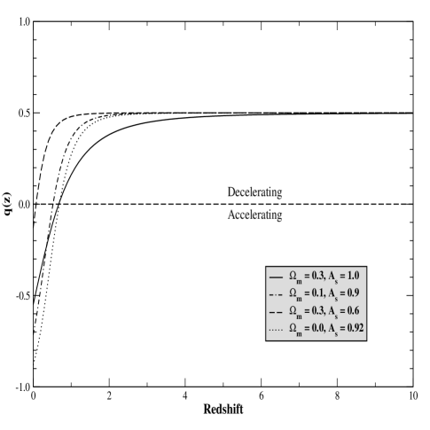
Figure 1: Deceleration parameter as a function of redshift for some selected values of $\Omega_{\rm{m}}$ and $A_{s}$. The horizontal line labeled decelerating/accelerating ($q_{o}=0$) divides models with a decelerating or accelerating expansion at a given redshift.

Figure 1 shows the behavior of the deceleration parameter as a function of redshift for selected values of $\Omega_{\rm{m}}$ and $A_{s}$. The best fit $\Lambda$CDM case is also showed for the sake of comparison ($A_{s}=1$). Note that the value of $A_{s}$ determines the acceleration redshift $z_{a}$. At late times, a CgCDM model with $\Omega_{\rm{m}}=0.1$ and $A_{s}=0.9$ accelerates faster than a $\Lambda$CDM scenario with $\Omega_{\rm{m}}=0.3$. In such a model the accelerated expansion begins at $z_{a}\simeq 0.51$. For the best fit model found in Ref. fabris , i.e., $\Omega_{\rm{m}}=0$ and $A_{s}=0.92$, the universe is strongly accelerated today with the accelerated phase begining at $z_{a}\simeq 0.68$ whereas for $A_{s}=1$ and $A_{s}=0.6$ and $\Omega_{\rm{m}}=0.3$ we find, respectively, $z_{a}\simeq 0.67$ and $z_{a}\simeq 0.07$.

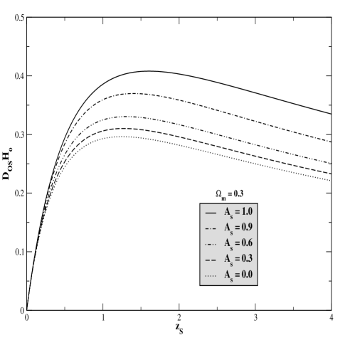
Figure 2: Dimensionless angular diameter distance as a function of the source redshift ($z_{S}$) for some selected values of $A_{s}$. In all curves the value of the matter density parameter has been fixed ($\Omega_{\rm{m}}=0.3$).

From Eqs. (2) and (5), it is straightforward to show that the comoving distance $r_{1}(z)$ to a light source located at $r=r_{1}$ and $t=t_{1}$ and observed at $r=0$ and $t=t_{o}$ can be written as

$$r_{1}(z)=\frac{1}{R_{o}H_{o}}\int_{x^{\prime}}^{1}{dx\over x^{2}f(x,\Omega_{\rm{m}},A_{s})},$$ (7)

where $x^{\prime}={R(t)\over R_{o}}=(1+z)^{-1}$ is a convenient integration variable and the dimensionless function $f(x,\Omega_{\rm{m}},A_{s})$ is given by

$$f(x,\Omega_{\rm{m}},A_{s})=\left[\frac{\Omega_{\rm{m}}}{x^{3}}+(1-\Omega_{\rm{m}})\sqrt{A_{s}+\frac{(1-A_{s})}{x^{6}}}\right]^{\frac{1}{2}}.$$ (8)

In order to derive the constraints from lensing statistics in Sec. IV we shall deal with the concept of angular diameter distance. For the class of models here investigated, the angular diameter distance, $D_{LS}(z_{L},z_{S})={R_{o}r_{1}(z_{L},z_{S})\over(1+z_{S})}$, between two objects, for example a lens at $z_{L}$ and a source (galaxy) at $z_{S}$, reads

$$D_{LS}(z_{L},z_{S}) = \frac{H_{o}^{-1}}{(1+z_{S})}\times$$

$$\times\int_{x^{\prime}_{S}}^{x^{\prime}_{L}}{dx\over x^{2}f(x,\Omega_{\rm{m}},A_{s})}.$$

In Fig. 2 we show the dimensionless angular diameter distance between an observer $O$ and the source $S$ ($D_{OS}H_{o}$) as a function of the source redshift ($z_{S}$) for $\Omega_{\rm{m}}=0.3$ and selected values of $A_{s}$. As physically expected, the larger the value of $A_{s}$ the larger the distance that is predicted between two redshifts. This result shows that, for the value of $\Omega_{\rm{m}}$ considered, the behaviour of this class of CgCDM models may be interpreted as an intermediary case between the $\Lambda$CDM ($A_{s}=1$) and the Einstein-de Sitter ($A_{s}=0$) scenarios. This particular feature of CgCDM models may be important for the lensing statistics analysis because, as is well known, the large distances predicted by $\Lambda$CDM models make the lensing constraints on the vaccum energy contribution very restrictive (see, for instance, 1CSK ). In this concern, we expect that the constraints from this particular test will be weaker for CgCDM scenarios than for their $\Lambda$CDM counterparts. It is worth mentioning that the behavior of CgCDM cosmology can be very different from that one present by $\Lambda$CDM scenarios and general quintessence cosmologies. For example, as shown in Ref. gorini , the trajectories of the statefinder parameters star in CgCDM scenarios differs considerably from the one presented by quintesence or $\Lambda$CDM models. As commented in gorini , the statefinder diagnostic combined with future supernovae observations (as, for example, the SNAP mission) may be able to discriminate between CgCDM and general quintessence cosmologies. More recently, an analysis for the location of the CMB peaks showed that CgCDM models and $\Lambda$CDM have very different predictions for large values of the parameter $A_{s}$ bento1 .

III The Age of the Universe

The predicted age of the Universe for the class of CgCDM models considered in this paper is given by

$$t_{o}=\frac{1}{H_{o}}\int^{1}_{0}{dx\over xf(x,\Omega_{\rm{m}},A_{s})}.$$ (10)

As widely known, a lower bound for this quantity can be estimated in a variety of different ways. For instance, Oswalt et al. osw , analyzing the cooling sequence of white dwarf stars found a lower age limit for the galactic disk of 9.5 Gyr. Later on, a value of 15.2 $\pm$ 3.7 Gyr was also determined using radioactive dating of thorium and europium abundances in stars cowan . In this connection, the recent age estimate of an extremely metal-poor star in the halo of our Galaxy (based on the detection of the 385.957 nm line of singly ionized ²³⁸U) indicated an age of 12.5 $\pm$ 3 Gyr cay . Another important way of estimating a lower limit to the age of the Universe is dating the oldest stars in globular clusters. Such estimates, however, have oscillated considerably since the publication of the statistical parallax measures done by Hipparcos. Initially, some studies implied in a lower limit of 9.5 Gyr at $95\%$ confidence level (c.l.) chab . Nevertheless, subsequent studies chab1 using new statistical parallax measures and updating some stellar model parameters, found 13.2 Gyr with a lower limit of 11 Gyr at 95$\%$ c.l., as a corrected mean value for age estimates of globular clusters (see also carreta ). Such a value implies that the Einstein-de Sitter model is ruled out for $h\geq 0.50$, while the most recent measurements of $h$ point consistently to $h\geq 0.65$ gio ; f1 . These results are also in accordance with recent estimates based on rather different methods for which the ages of the oldest globular clusters in our Galaxy fall on the interval 13.8 - 16.3 Gyr rengel .

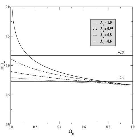
Figure 3: $H_{o}t_{o}$ as a function of the matter density parameter for some values of $A_{s}$. Horizontal lines correspond to $\pm 2\sigma$ limits of the age parameter $H_{o}t_{o}=0.95\pm 0.11$.

By assuming $t_{o}=13\pm 1$ Gyr as a median value for the most recent age estimates of globular clusters and $H_{o}=72\pm 8$ ${\rm{Km.s^{-1}.Mpc^{-1}}}$, in accordance with the final results of the Hubble Space Telescope Key Project f1 , we find $H_{o}t_{o}=0.95\pm 0.11$, a value that is compatible with the estimates discussed above, as well as very close to some determinations based on SNe Ia data riess ; tonry . In Fig. 3 we show the dimensionless age parameter $H_{o}t_{o}$ as a function of $\Omega_{\rm{m}}$ for some selected values of $A_{s}$. Horizontal dashed lines indicate $\pm 2\sigma$ of the age parameter for the values of $H_{o}$ and $t_{o}$ considered here. Similarly to the discussion for the angular diameter distance, for a fixed value of $\Omega_{\rm{m}}$ the predicted age of the Universe is larger for larger values of $A_{s}$. If $\Omega_{\rm{m}}=0.2-0.4$, as sugested by dynamical estimates on scales up to about $2h^{-1}$ Mpc calb , we find $A_{s}\geq 0.96$ (see also jailn ).

IV Constraints from Lensing Statistics

In order to constrain the parameters $\Omega_{\rm{m}}$ and $A_{s}$ from lensing statistics we work with a sample of 867 ($z>1$) high luminosity optical quasars which includes 5 lensed quasars. This sample consists of data from the following optical lens surveys: HST Snapshot survey HST , Crampton survey Crampton , Yee survey Yee , Surdej survey Surdej , NOT Survey Jaunsen and FKS survey FKS .

The differential probability $d\tau$ of a beam having a lensing event in traversing $dz_{L}$ is TOG ; FFKT

$$d\tau=F^{*}(1+z_{L})^{3}\left({D_{OL}D_{LS}\over R_{0}D_{OS}}\right)^{2}{1\over R_{0}}{dt\over dz_{L}}dz_{L},$$ (11)

where

$${dt\over dz_{L}}={H_{o}^{-1}\over(1+z_{L})f(x,\Omega_{\rm{m}},A_{s})},$$ (12)

and

$$F^{*}={16\pi^{3}\over{cH_{0}^{3}}}\phi_{\ast}v_{\ast}^{4}\Gamma\left(\alpha+{4\over\gamma}+1\right).$$ (13)

In Eq. (11), $D_{OL}$, $D_{OS}$ and $D_{LS}$ are, respectively, the angular diameter distances from the observer to the lens, from the observer to the source and between the lens and the source. We use the Schechter luminosity function with the lens parameters for E/SO galaxies taken from Madgwick et al. Mad , i.e., $\phi_{\ast}=0.27h^{3}\,10^{-2}{\rm{Mpc}}^{-3}$, $\alpha=-0.5$, $\gamma=4$, $v_{\ast}=220\,{\rm{km/s}}$ and $F^{*}=0.01$.

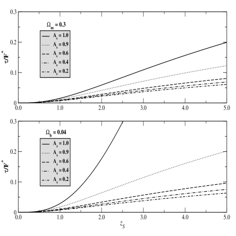
Figure 4: The normalized optical depth ($\tau/F^{*}$) as a function of the source redshift ($z_{S}$) for some selected values of $A_{s}$. Upper panel: CgCDM models with $\Omega_{\rm{m}}=0.3$. Lower panel: a universe dominated by baryonic matter ($\Omega_{b}=0.04$) and the Chaplygin gas.

The total optical depth is obtained by integrating $d\tau$ along the line of sight from $z_{O}$ ($z=0$) to $z_{S}$. One obtains

$$\tau(z_{S})=\frac{F^{*}}{30}\left[D_{OS}(1+z_{L})\right]^{3}\,R_{o}^{3}.$$ (14)

In Fig. 4 we show the normalized optical depth as a function of the source redshift ($z_{S}$) for values of $A_{s}=$ 0.2, 0.4, 0.6, 0.9 and 1.0. Two different cases are illustrated: a conventional CgCDM model with the matter density parameter fixed at $\Omega_{\rm{m}}=0.3$ and a Chaplygin gas + baryonic matter model with $\Omega_{b}=1-\Omega_{Cg}=0.04$. As discussed earlier, the reason for considering the later case is because one of the strongest claims for a Chaplygin gas dark energy is the possibility of a unified explanation for the dark matter and dark energy problems bilic . In this case, one might expect that the only two components of the Universe would be the Chaplygin gas and the baryonic matter. Note that in both cases an increase in $A_{s}$ at fixed $\Omega_{\rm{m}}$ tends to increase the optical depth for lensing. For example, for $\Omega_{\rm{m}}=0.3$, the value of $\tau/F^{*}$ for $A_{s}=0.2$ at $z_{S}=3.0$ is down from the $\Lambda$CDM ($A_{s}=1$) value by a factor of $\sim$ 2.97, while at the same redshift, $\tau/F^{*}$ for $A_{s}=0.4$ is down from that for $A_{s}=1.0$ by $\sim$ 2.63. By fixing the value of $A_{s}$, for example, $A_{s}=0.6$, we observe that the value of $\tau/F^{*}$ is smaller for a universe with $\Omega_{\rm{m}}=0.3$ than for a universe composed only of the Chaplygin gas + baryonic matter ($\Omega_{b}=0.04$) by a factor of $\sim$ 1.18. This increase of the optical depth as the value of $A_{s}$ is increased (at a fixed $z_{S}$ and $\Omega_{\rm{m}}$) is an expected consequence since this model more closely approaching the $\Lambda$CDM case as $A_{S}\rightarrow 1$.

The likelihood function is defined by

$${\cal{L}}=\prod_{i=1}^{N_{U}}(1-p^{{}^{\prime}}_{i})\,\prod_{k=1}^{N_{L}}p_{k}^{{}^{\prime}}\,p_{ck}^{{}^{\prime}},$$ (15)

where $N_{L}$ is the number of multiple-imaged lensed quasars, $N_{U}$ is the number of unlensed quasars, and $p_{k}^{{}^{\prime}}$ and $p_{ck}^{i}$ are, respectively, the probability of quasar $k$ to be lensed and the configuration probability. These quantities are defined by

$$p^{{}^{\prime}}_{i}(m,z)=p_{i}\int\frac{d(\Delta\theta)\,p_{c}(\Delta\theta)\emph{B}(m,z,M_{f}(\Delta\theta),M_{2})}{\emph{B}(m,z,M_{0},M_{2})}$$ (16)

and

$$p^{{}^{\prime}}_{ci}=p_{ci}(\Delta\theta)\,\frac{p_{i}}{p_{i}^{{}^{\prime}}}\,\frac{\emph{B}(m,z,M_{f}(\Delta\theta),M_{2})}{\emph{B}(m,z,M_{0},M_{2})},$$ (17)

where

$$p_{c}(\Delta\theta)=\frac{1}{\tau(z_{S})}\,\int_{0}^{z_{S}}\frac{d^{2}\tau}{dz_{L}d(\Delta\theta)}\,dz_{L}$$ (18)

and

$$M_{f}=M_{0}(f+1)/(f-1)\quad\mbox{with}\quad f=10^{0.4\,\Delta m(\theta)}.$$ (19)

The magnification bias, ${\bf B}(m,z)$, is considered in order to take into account the increase in the apparent brightness of a quasar due to lensing which, in turn, increases the expected number of lenses in flux limited sample. The bias factor for a quasar at redshift $z$ with apparent magnitude $m$ is given by FFKT ; 1CSK

$${\bf B}(m,z)=M_{0}^{2}\,\emph{B}(m,z,M_{0},M_{2}),$$ (20)

where

$$\emph{B}(m,z,M_{1},M_{2}) = 2\,\left(\frac{dN_{Q}}{dm}\right)^{-1}\int_{M_{1}}^{M_{2}}\frac{dM}{M^{3}}\,$$

$$\times\,\frac{dN_{Q}}{dm}(m+2.5\log(M),z).$$

In the above equation $({dN_{Q}(m,z)}/{dm})$ is the measure of number of quasars with magnitudes in the interval $(m,m+dm)$ at redshift $z$. Since we are modeling the lens by a singular isothermal model profile, $M_{0}=2$, we adopt $M_{2}=10^{4}$ in the numerical computation.

For the quasar luminosity function we use Kochanek’s “best model” 1CSK

$$\frac{dN_{Q}}{dm}(m,z)\propto(10^{-a(m-\overline{m})}+10^{-b(m-\overline{m})})^{-1},$$ (22)

where

$$\overline{m}=\left\{\begin{array}[]{ll}m_{o}+(z-1)&\mbox{for $z<1$}\\ m_{o}&\mbox{for $1<z\leq 3$}\\ m_{o}-0.7(z-3)&\mbox{for $z>3$}\end{array}\right.\$$ (23)

and we assume $a=1.07\pm 0.07$, $b=0.27\pm 0.07$ and $m_{o}=18.92\pm 0.16$ at B magnitude 1CSK .

Due to selection effects the survey can detect lenses with magnification larger than a certain magnitude $M_{f}$ given by equation (19) which becomes the lower limit in equation (IV). To obtain selection function corrected probabilities, we follow 1CSK and divide our sample into two parts, namely, the ground based surveys and the HST survey.

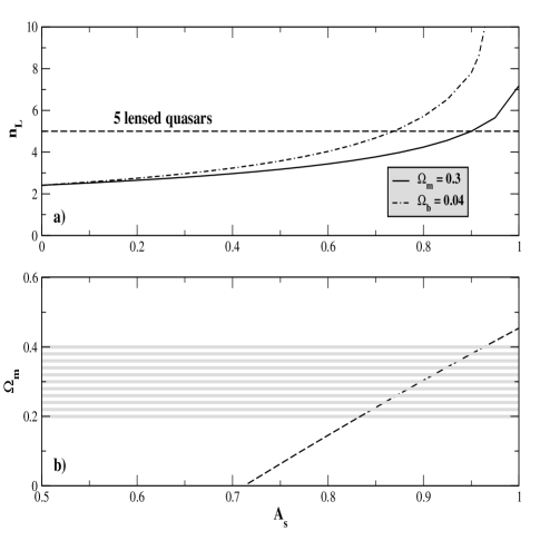
Figure 5: a) Predicted number of lensed quasars as a function of $A_{s}$ for $\Omega_{\rm{m}}=0.3$ (solid line) and $\Omega_{b}=0.04$ (dashed-dotted line) and image separation $\Delta\theta\leq 4$. b) Contour for five lensed quasars in the parametric space $A_{s}-\Omega_{\rm{m}}$. The shadowed horizontal region corresponds to the observed range $\Omega_{\rm{m}}=0.3\pm 0.1$ calb .

From Eq. (15) we find that the maximum value of the likelihood function is located at $\Omega_{\rm{m}}=0.4$ and $A_{s}=1.0$. At the 1$\sigma$ level, however, almost the entire range of $A_{s}$ is compatible with the observational data for values of $\Omega_{\rm{m}}=0-1$. As observed earlier (see Sec. II), this result suggests that a large class of CgCDM scenarios is in accordance with the current gravitational lensing data. For the sake of comparison, we also analyse some possible differences between our best-fit value and the one obtained for general quintessence scenarios with an equation of state $p_{x}=\omega_{x}\rho_{x}$ (XCDM) turner . For example, for XCDM models a similar analysis shows that the maximum value of the likelihood function is located at $\Omega_{\rm{m}}=0.0$ and $\omega_{x}=-0.2$ waga . Such a model corresponds to a decelerated universe with a deceleration parameter $q_{o}=0.2$ and a total expanding age of $8.1h^{-1}$ Gyr while our best-fit CgCDM model corresponds to an accelerating scenario with $q_{o}=-0.39$ ($z_{a}=0.44$) and a total age of the order of $8.7h^{-1}$ Gyr. In Fig. 5a the expected number of lensed quasars, $n_{L}=\sum\,p_{i}^{{}^{\prime}}$ (the summation is over a given quasar sample), is displayed as a function of $A_{s}$. As indicated in the figure, the horizontal dashed line indicates $n_{L}=5$, that is the number of lensed quasars in our sample. By this analysis, one finds $A_{s}=0.9$ ($\Omega_{\rm{m}}=0.3$) and $A_{s}=0.73$ ($\Omega_{b}=0.04$). In Fig. 3b we show the contour for five lensed quasars in the parametric space $A_{s}-\Omega_{\rm{m}}$. The shadowed horizontal region corresponds to the observed range $\Omega_{\rm{m}}=0.3\pm 0.1$ calb . As a general result, this analysis provides $\Omega_{\rm{m}}\leq 0.45$ and $A_{s}\geq 0.72$. We also observe that the higher the value of $\Omega_{\rm{m}}$ the higher the value of $A_{s}$ that is required to fit these data.

V Conclusion

The search for alternative cosmologies is presently in vogue and the leitmotiv is the observational support for an accelerated universe provided by the SNe Ia results. In general, such alternative scenarios contain an unkown negative-pressure dark component that explains the SNe Ia results and reconciles the inflationary flatness prediction ($\Omega_{\rm{T}}=1$) with the dynamical estimates of the quantity of matter in the Universe ($\Omega_{\rm{m}}\simeq 0.3\pm 0.1$). In this paper we have focused our attention on another dark energy candidate: the Chaplygin gas. We showed that the predicted age of the Universe in the context of CgCDM models is compatible with the most recent age estimates of globular clusters for values of $\Omega_{\rm{m}}\simeq 0.2$ and $A_{s}\geq 0.96$. We also studied the influence of such a component on the statistical properties of gravitational lensing. At $1\sigma$ level we found that a large class of these scenarios is in agreement with the current lensing data with the maximum of the likelihood function (Eq. 15) located at $\Omega_{\rm{m}}=0.4$ and $A_{s}=1.0$. As a general result, the predicted number of lensed quasars requires $\Omega_{\rm{m}}\leq 0.45$ and $A_{s}\geq 0.72$.

- (1) B. Ratra and P. J. E. Peebles, Phys. Rev. D37, 3406 (1988); J. A. Frieman, C. T. Hill, A. Stebbins and I. Waga, Phys. Rev. Lett. 75, 2077 (1995); R. R. Caldwell, R. Dave and P. J. Steinhardt, Phys. Rev. Lett. 80, 1582 (1998); T. D. Saini, S. Raychaudhury, V. Sahni and A. A. Starobinsky, Phys. Rev. Lett. 85, 1162 (2000)
- (2) M. S. Turner and M. White, Phys. Rev. D56, R4439 (1997); T. Chiba, N. Sugiyama and T. Nakamura, Mon. Not. Roy. Astron. Soc. 289, L5 (1997); S. A. Bludman and M. Roos Astrophys. J. 547,77 (2001); J. A. S. Lima and J. S. Alcaniz, Astrophys. J. 566, 15 (2002); R. Bean and A. Melchiorri, Phys. Rev. D65, 041302(R) (2002); D. Jain et al., astro-ph/0105551; J. Kujat et al., Astrophys. J. 572, 1 (2002); P. J. E. Peebles and B. Ratra, astro-ph/0207347
- (3) M. Ozer and M. O. Taha Phys. Lett. B171, 363 (1986); Nucl. Phys. B287, 776 (1987); O. Bertolami, Nuovo Cimento, B93, 36 (1986); K. Freese, F. C. Adams, J. A. Frieman and E. Mottola, Nucl. Phys. B287, 797 (1987); W. Chen and Y.-S. Wu, Phys. Rev. D41, 695 (1990); J. C. Carvalho, J. A. S. Lima and I. Waga, Phys. Rev. D46 2404 (1992); J. M. Salim and I. Waga, Class. Quant, Grav. 10, 1767 (1993); I. Waga, Astrophys. J. 414, 436 (1993); J. A. S Lima and J. M. F. Maia, Phys. Rev. D49, 5597 (1994); J. A. S. Lima and M. Trodden, Phys. Rev. D53, 4280 (1996); F. M. Overduin and F. I. Cooperstock, Phys. Rev. D58, 043506 (1998); O. Bertolami and P. J. Martins, Phys. Rev. D61, 064007 (2000); R. G. Vishwakarma, Gen. Rel. Grav. 33, 1973 (2001)
- (4) L. Randall and R. Sundrum, Phys. Rev. Lett. 83, 3370 (1999); G. Dvali, G. Gabadadze and M. Porrati, Phys. Lett. B485, 208 (2000); C. Deffayet, Phys. Lett. B 502, 199 (2001); R. Dick, Class. Quant. Grav. 18, R1 (2001); J. S. Alcaniz, Phys. Rev. D 65, 123514 (2002); V. Sahni and Y. Shtanov, astro-ph/0202346; M. D. Maia, E. M. Monte, J. M. F. Maia, astro-ph/0208223; A. Lue, hep-th/0208169
- (5) A. Kamenshchik, U. Moschella and V. Pasquier, Phys. Lett. B511, 265 (2001)
- (6) M. S. Turner, Phys. Rept. 333, 619 (2000)
- (7) R. R. Caldwell, Braz. J. Phys. 30, 215 (2000)
- (8) J. V. Cunha, J. S. Alcaniz and J. A. S. Lima, Phys. Rev. D 66, 023520 (2002)
- (9) C. Deffayet, S. J. Landau, J. Raux, M. Zaldarriaga and P. Astier, Phys. Rev. D66, 024019 (2002) ; D. Jain, J. S. Alcaniz and A. Dev, Phys. Rev. D66, 083511 (2002); J. S. Alcaniz, A. Dev and D. Jain, Phys Rev. D66, 067301 (2002)
- (10) M. Bordemann and J. Hoppe, Phys. Lett. B 317, 315 (1993)
- (11) R. Jackiw, “(A Particle Field Theorist’s) Lecture on (Supersymmetric Non-Abelian) Fluid Mechanics (and -branes)”, physics/0010042
- (12) N. Bilić, G. B. Tupper and R. D. Viollier, Phys. Lett. B 535, 17 (2002); N. Bilić, G. B. Tupper and R. D. Viollier, astro-ph/0207423
- (13) J. C. Fabris, S. V. B. Goncalves and P. E. de Souza, Gen. Rel. Grav. 34, 53 (2002)
- (14) M. C. Bento, O Bertolami and A. A. Sen, Phys. Rev. D66, 043507 (2002)
- (15) J. C. Fabris, S. V. B. Goncalves and P. E. de Souza, astro-ph/0207430
- (16) P. P. Avelino, L. M. G. Beça, J. P. M. de Carvalho, C. J. A. P. Martins and P. Pinto, astro-ph/0208528
- (17) M. C. Bento, O. Bertolami and A. A. Sen, astrp-ph/0210468
- (18) C. S. Kochaneck, Astrophys. J. 466, 638 (1996)
- (19) V. Gorini, A. Kamenshchik and U. Moschella, astro-ph/0209395
- (20) V. Sahni, T. D. Saini, A. A. Starobinsky, U. Alam, astro-ph/0201498
- (21) T. D. Oswalt, J. A. Smith, M. A. Wood and P. Hintzen, Nature 382, 692 (1996)
- (22) J. J. Cowan et al., Astrophys. J. 480, 246 (1997)
- (23) R. Cayrel et al., Nature 409, 691 (2001).
- (24) Chaboyer B., Demarque P. and Kernan P.J. et al., Astrophys. J. 494, 96 (1998)
- (25) L. M. Krauss, Phys. Rept. 333, 33 (2000); L. M. Krauss and B. Chaboyer, astro-ph/0111597
- (26) E. Carretta et al., Astrophys. J. 533, 215 (2000).
- (27) R. Giovanelli et al. Astrophys. J. 477, L1 (1997)
- (28) W. L. Freedman et al., Astrophys. J. 553, 47 (2001)
- (29) M. Rengel, J. Mateu and G. Bruzual, IAU Symp. 207, Extragalactic Star Clusters, Eds. E. Grebel, D. Geisler, D Minnite (in Press), astro-ph/0106211 (2002).
- (30) A. Riess et al., Astron. J. 116, 1009 (1998)
- (31) J. L. Tonry, astro-ph/0105413
- (32) R. G. Calberg et al., Astrophys. J. 462, 32 (1996); A. Dekel, D. Burstein and S. White S., In Critical Dialogues in Cosmology, edited by N. Turok World Scientific, Singapore (1997)
- (33) J. S. Alcaniz, A. Dev and D. Jain, astro-ph/0210476
- (34) D. Maoz et al., Astrophys. J. , 409, 28 (1993)
- (35) D. Crampton, R. McClure and J. M. Fletcher, Astrophys. J. 392, 23 (1992)
- (36) H. K. C. Yee, A. V. Filippenko and D. Tang, Astron. J. 105, 7 (1993)
- (37) J. Surdej et al., Astron. J. 105, 2064 (1993)
- (38) A. O. Jaunsen, M. Jablonski, B. R. Petterson and R. Stabell, Astron. Astrop., 300, 323 (1995)
- (39) C. S. Kochanek, E. E. Falco, and R. Schild, Astrophys. J. 452, 109 (1995)
- (40) M. Fukugita, T. Futamase, M. Kasai and E. L. Turner, Astrophys. J. 393, 3 (1992)
- (41) E. L. Turner, J. P. Ostriker and J. R. Gott III, Astrophys. J. 284, 1 (1984)
- (42) D. S. Madgwick et al., astro-ph/0107197
- (43) I. Waga and A. P. M. R. Miceli, Phys. Rev. D 59, 103507 (1999)