Evolution characteristics of central black hole of magnetized accretion disc

Abstract

Evolution characteristics of a Kerr black hole (BH) are investigated by considering coexistence of disc accretion with the Blandford-Znajek process (the BZ process) and magnetic coupling of the BH with the surrounding disc (MC process). (i) The rate of extracting energy from the rotating BH in the BZ process and that in MC process are expressed by a unified formula, which is derived by using an improved equivalent circuit. (ii) The mapping relation between the angular coordinate on the BH horizon and the radial coordinate on the disc is given in the context of general relativity and conservation of magnetic flux. (iii) The power and torque in the BZ process are compared with those in MC process in detail. (iv) Evolution characteristics of the BH and energy extracting efficiency are discussed by using the characteristics functions of BH evolution in the corresponding parameter space. (v) Power dissipation on the BH horizon and BH entropy increase are discussed by considering the coexistence of the above energy mechanisms.

1 Introduction

It is well known that magnetized accretion disc of black hole (BH) is an effective model in astrophysics. The interaction between a Kerr BH and the surrounding magnetic field has been used not only to explain high energy radiation and jet production from quasars and active galactic nuclei, but also as a possible central engine for gamma-ray bursts (Rees 1984; Frank, King & Raine 1992; Lee, Wijers & Brown 2000, hereafter LWB). Confined by the magnetic field in the inner region of the disc, the magnetic field lines frozen previously in the disc plasma will deposit on the horizon in company with the accretion onto the BH, and the magnetized disc becomes a good environment for supporting the magnetic field on the horizon. Blandford and Znajek (1977) proposed firstly that the rotating energy and the angular momentum of a BH can be extracted by the surrounding magnetic field, and this energy mechanism has been referred to as the BZ process, in which the BH horizon and the remote astrophysical load are connected by the open magnetic field lines, and energy and angular momentum are extracted from the rotating BH and transported to the remote load.
There still remain some open problems on the BZ process, and one of them is how to estimate the ratio of the angular velocity of the magnetic field lines to that of the BH horizon. Macdonald and Thorne (1982 hereafter MT82) argued in a speculative way that the ratio will be regulated to about 0.5 by the BZ process itself, which corresponds to the optimal value of the extracting power with the impedance matching. However, as argued by Punsly and Coroniti (1990), it is hard to understand how the load can conspire with the BH to have the same resistance and satisfy the matching condition, since the load is so far from the BH that it cannot be casually connected.
Recently some authors (Blandford 1999; Li 2000a, 2000b; Li & Paczynski 2000) argued that with the existence of the closed field lines a fast rotating BH will exert a torque on the disc to transfer energy and angular momentum from the BH to the disc. Henceforce this energy mechanism is referred to as magnetic coupling (MC) process. Compared with the BZ process, the load in MC process is the surrounding disc, which is much better understood than the remote load though the magnetohydrodynamics (MHD) of the disc is still very complicated.
Some works have been done to discuss the influence of the BZ process on the evolution of BH accretion disc (Park & Vishniac 1988; Moderski & Sikora 1996; Lu et al. 1996; Wang et al. 1998, hereafter WLY). However MC effects involving the closed field lines were not taken into account in the previous works. In fact the closed field lines should exist on the horizon as well as the open field lines, and disc accretion should coexist with the BZ and MC process. In this paper evolution characteristics of a Kerr BH are investigated by considering coexistence of disc accretion with the BZ and MC process (henceforce DABZMC).
In order to facilitate the discussion of the evolution of the central BH surrounded by the magnetized accretion disc we make the following assumptions:
(i) The disc is perfectly conducting and the magnetic field lines are frozen in the disc. The magnetosphere is stationary, axisymmetric and force-free outside the BH and the disc (MT82);
(ii) The magnetic field is so weak that its influence on the dynamics of the particles in the disc is negligible, and the BH has an external geometry of Kerr metric;
(iii) The disc is thin and Keplerian, lies in the equatorial plane of the BH with the inner boundary being at the marginally stable orbit.
This paper is organized as follows. In Sec.II the rate of extracting energy from the rotating BH in the BZ process (henceforce the BZ power) and that in MC process (henceforce MC power) are expressed by a unified formula, which is derived by using an improved equivalent circuit based on MT82. Our result for the BZ power is consistent with that derived in LWB. In Sec.III a mapping relation between the angular coordinate on the BH horizon and the radial coordinate on the disc is given in the context of general relativity and conservation of magnetic flux. In Sec.IV The power and torque in the BZ process are compared with those in MC process in detail. In Sec.V evolution characteristics of the BH and energy extracting efficiency are discussed by using the characteristics functions in the corresponding parameter space. In Sec.VI we discuss the power dissipation on the BH horizon and the BH entropy increase, and show that the excess rate of change of BH entropy does come from the total power dissipation on the BH horizon in the BZ and MC process. Finally, in Sec.VII, we summarize our main results.

2 DERIVATION OF BZ POWER AND MC POWER

Two mechanisms of magnetic extraction of energy from a rotating BH are involved in our model, i.e., the BZ process and MC process. The configuration of the poloidal magnetic field of the BH magnetosphere for the coexistence of DABZMC is shown in Fig.1, where the angular coordinate of the open field lines is assumed to vary from $0$ to $\theta_{M}$, and that of the closed field lines from $\theta_{M}$ to $\pi/2$. $\theta_{M}$ is a parameter indicating the angular boundary between the open and the closed field lines, and the BZ and MC effects vanish as $\theta_{M}=0$ and $\theta_{M}=\pi/2$ , respectively.

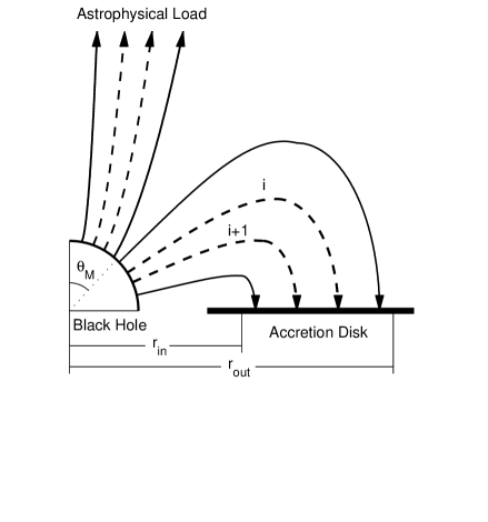
Figure 1: The configuration of the poloidal magnetic field of the BH magnetosphere.

Considering that both mechanisms arise from the rotation of the Kerr BH relative to the surrounding magnetic field, we expect that the BZ power and MC power can be expressed by a unified formula. In order to do this we proposed a model, in which the remote load in the BZ process and the load disc in MC process are incorporated into a unified load with resistance $Z_{L}$ and angular velocity $\Omega_{L}$ . Based on MT82 an improved equivalent circuit is shown in Fig.2, in which a series of loops correspond to the adjacent magnetic surfaces consisting of the field lines connecting the BH horizon and the load.

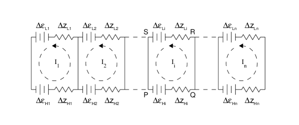
Figure 2: An improved equivalent circuit for a unified model for the BZ and MC process.

In the i-loop of Fig.2 segments $PS$ (characterized by the flux $\Psi$) and $QR$ (characterized by the flux $\Psi+\Delta\Psi$) represent two adjacent magnetic surfaces, and segments $PQ$ and $RS$ represent the BH horizon and the load sandwiched by the two surfaces. $\Delta Z_{H}$ and $\Delta Z_{L}$ (hereafter subscript ”i” is omitted) are the corresponding resistances of the BH horizon and the load, respectively. $\Delta\varepsilon_{H}=(\Delta\Psi/2\pi)\Omega_{H}$ and $\Delta\varepsilon_{L}=-(\Delta\Psi/2\pi)\Omega_{L}$ are electromotive forces due to the rotation of the BH and the load, respectively. The minus sign in the expression of $\Delta\varepsilon_{L}$ arises from the direction of the flux. $\Omega_{H}$ in the expression of $\Delta\varepsilon_{H}$ is the angular velocity of the BH horizon and reads (G=c=1):

$$\Omega_{H}=a_{*}/(2r_{H}),r_{H}=M\left({1+q}\right),q=\sqrt{1-a_{*}^{2}}$$ (1)

where $a_{*}$ is the BH spin, which is related to BH mass $M$ and angular momentum $J$ by $a_{*}\equiv J/M^{2}$, and $r_{H}$ is the radius of the BH horizon. By using the BH magnetosphere model given in MT82 we obtain the following equations:

$$\begin{array}[]{l}\int_{P}^{Q}{\alpha\vec{E}\cdot d\vec{l}}=\Delta V_{H}=\left({{{\Delta\Psi}\mathord{\left/{\vphantom{{\Delta\Psi}{2\pi}}}\right.\kern-1.2pt}{2\pi}}}\right)\left({\omega_{H}-\Omega_{F}}\right)\\ =\left({{{\Delta\Psi}\mathord{\left/{\vphantom{{\Delta\Psi}{2\pi}}}\right.\kern-1.2pt}{2\pi}}}\right)\left({\Omega_{H}-\Omega_{F}}\right)=I\Delta Z_{H}\\ \end{array}$$ (2)

$$\begin{array}[]{l}\int_{R}^{S}{\alpha\left({\vec{E}+\vec{\upsilon}_{L}\times\vec{B}}\right)\cdot d\vec{l}}=\Delta V_{L}+\left({{{\Delta\Psi}\mathord{\left/{\vphantom{{\Delta\Psi}{2\pi}}}\right.\kern-1.2pt}{2\pi}}}\right)\left({\omega_{L}-\Omega_{L}}\right)\\ =\left({{{\Delta\Psi}\mathord{\left/{\vphantom{{\Delta\Psi}{2\pi}}}\right.\kern-1.2pt}{2\pi}}}\right)\left({\Omega_{F}-\Omega_{L}}\right)=I\Delta Z_{L}\\ \end{array}$$ (3)

$$\Delta V_{L}=\int_{R}^{S}{\alpha\vec{E}\cdot d\vec{l}}=\left({{{\Delta\Psi}\mathord{\left/{\vphantom{{\Delta\Psi}{2\pi}}}\right.\kern-1.2pt}{2\pi}}}\right)\left({\Omega_{F}-\omega_{L}}\right)$$ (4)

where $\Delta V_{H}$ and $\Delta V_{L}$ are the potential drops measured by ”zero-angular-momentum observers” (ZAMOs) on the BH horizon and on the load, respectively. ZAMOs is a family of fiducial observers defined by Bardeen et al (1972). $\vec{\upsilon}_{L}$ is the load’s velocity relative to ZAMOs. $\omega_{H}\left({\to\Omega_{H}}\right)$ and $\omega_{L}$ are the ZAMO angular velocities on the BH horizon and the load, respectively. $\Omega_{F}$ is the angular velocity of the magnetic field lines. $\alpha\equiv\left({{{d\tau}\mathord{\left/{\vphantom{{d\tau}{dt}}}\right.\kern-1.2pt}{dt}}}\right)_{ZAMO}$ is the ”lapse function”, which is written as follows:

$$\alpha={{\rho\sqrt{\Delta}}\mathord{\left/{\vphantom{{\rho\sqrt{\Delta}}\Sigma}}\right.\kern-1.2pt}\Sigma}$$ (5)

where $\Sigma$, $\rho$ and $\Delta$ are the Kerr metric parameters and read

$$\Sigma^{2}\equiv\left({r^{2}+a^{2}}\right)^{2}-a^{2}\Delta\sin^{2}\theta,\rho^{2}\equiv r^{2}+a^{2}\cos^{2}\theta$$

$$\Delta\equiv r^{2}+a^{2}-2Mr$$ (6)

Incorporating equations (2) and (3) we obtain

$$\Delta\varepsilon_{H}+\Delta\varepsilon_{L} = \int_{P}^{Q}{\alpha\vec{E}\cdot d\vec{l}}+\int_{R}^{S}{\alpha\left({\vec{E}+\vec{\upsilon}_{L}\times\vec{B}}\right)\cdot d\vec{l}}$$ (7)

$$= I\left({\Delta Z_{H}+\Delta Z_{L}}\right)$$

Dividing equation (2) by equation (3), we derive the relation relating the three angular velocities, $\Omega_{H}$, $\Omega_{L}$ and $\Omega_{F}$ as follows:

$$\Omega_{F}={{\left({\Omega_{H}\Delta Z_{L}+\Omega_{L}\Delta Z_{H}}\right)}\mathord{\left/{\vphantom{{\left({\Omega_{H}\Delta Z_{L}+\Omega_{L}\Delta Z_{H}}\right)}{\left({\Delta Z_{H}+\Delta Z_{L}}\right)}}}\right.\kern-1.2pt}{\left({\Delta Z_{H}+\Delta Z_{L}}\right)}}$$ (8)

Assuming $\Omega_{L}=0$ in the BZ process, we have

$$\Omega_{F}={{\Omega_{H}\Delta Z_{L}}\mathord{\left/{\vphantom{{\Omega_{H}\Delta Z_{L}}{\left({\Delta Z_{H}+\Delta Z_{L}}\right)}}}\right.\kern-1.2pt}{\left({\Delta Z_{H}+\Delta Z_{L}}\right)}}$$ (9)

Considering that the load disc consists of plasma of perfect conductivity and the magnetic field lines are frozen in the disc plasma, we have $\Delta Z_{L}=0$ and

$$\Omega_{F}=\Omega_{L}=\Omega_{D}=\frac{1}{{M(\chi^{3}+a_{*})}}$$ (10)

where $\Omega_{D}$ is the angular velocity of the disc at the place where the magnetic flux penetrates, and $\chi=\sqrt{r/M}$ is dimensionless radial coordinate of the disc. The current $I$ in each loop can be expressed by

$$I = \frac{{\Delta\varepsilon_{H}+\Delta\varepsilon_{L}}}{{\Delta Z_{H}+\Delta Z_{L}}}=\left({{{\Delta\Psi}\mathord{\left/{\vphantom{{\Delta\Psi}{2\pi}}}\right.\kern-1.2pt}{2\pi}}}\right)\frac{{\Omega_{H}-\Omega_{L}}}{{\Delta Z_{H}+\Delta Z_{L}}}$$ (11)

$$= \left({{{\Delta\Psi}\mathord{\left/{\vphantom{{\Delta\Psi}{2\pi}}}\right.\kern-1.2pt}{2\pi}}}\right)\frac{{\Omega_{H}-\Omega_{F}}}{{\Delta Z_{H}}}$$

where equation (8) is used in deriving the right-hand side (RHS) of equation (11). The current $I$ on the BH horizon feels Ampere’s force, and the torque exerted on the annular ring of the width $\Delta l=\rho\Delta\theta$ is

$$\Delta T=\varpi B_{H}I\Delta l=\left({{{\Delta\Psi}\mathord{\left/{\vphantom{{\Delta\Psi}{2\pi}}}\right.\kern-1.2pt}{2\pi}}}\right)^{2}{{\left({\Omega_{H}-\Omega_{F}}\right)}\mathord{\left/{\vphantom{{\left({\Omega_{H}-\Omega_{F}}\right)}{\Delta Z_{H}}}}\right.\kern-1.2pt}{\Delta Z_{H}}}$$ (12)

where $\Delta\Psi=B_{H}2\pi\varpi\Delta l$, $B_{H}$ is the magnetic field on the horizon, and $\varpi=\left({{\Sigma\mathord{\left/{\vphantom{\Sigma\rho}}\right.\kern-1.2pt}\rho}}\right)\sin\theta$ is the cylindrical radius of the horizon. Therefore the extracting power between the two adjacent magnetic surfaces is

$$\Delta P=\Omega_{F}\Delta T=\left({{{\Delta\Psi}\mathord{\left/{\vphantom{{\Delta\Psi}{2\pi}}}\right.\kern-1.2pt}{2\pi}}}\right)^{2}{{\Omega_{F}\left({\Omega_{H}-\Omega_{F}}\right)}\mathord{\left/{\vphantom{{\Omega_{F}\left({\Omega_{H}-\Omega_{F}}\right)}{\Delta Z_{H}}}}\right.\kern-1.2pt}{\Delta Z_{H}}}$$ (13)

where

$$\Delta Z_{H}=R_{H}{{\Delta l}\mathord{\left/{\vphantom{{\Delta l}{\left({2\pi\varpi}\right)}}}\right.\kern-1.2pt}{\left({2\pi\varpi}\right)}}={{2\rho\Delta\theta}\mathord{\left/{\vphantom{{2\rho\Delta\theta}\varpi}}\right.\kern-1.2pt}\varpi}$$ (14)

and $R_{H}=4\pi/c=377ohm$ is the surface resistivity of the BH horizon. Considering that the BH horizon consists of two hemispheres and integrating equations (13) and (12) over the angular coordinate from $\theta=0$ to $\theta_{M}$ we obtain the total BZ power and torque as follows:

$${{P_{BZ}}\mathord{\left/{\vphantom{{P_{BZ}}{P_{0}}}}\right.\kern-1.2pt}{P_{0}}}=2a_{*}^{2}\int_{0}^{\theta_{M}}{\frac{{k\left({1-k}\right)\sin^{3}\theta d\theta}}{{2-\left({1-q}\right)\sin^{2}\theta}}}$$ (15)

$${{T_{BZ}}\mathord{\left/{\vphantom{{T_{BZ}}{T_{0}}}}\right.\kern-1.2pt}{T_{0}}}=4a_{*}\left({1+q}\right)\int_{0}^{\theta_{M}}{\frac{{\left({1-k}\right)\sin^{3}\theta d\theta}}{{2-\left({1-q}\right)\sin^{2}\theta}}}$$ (16)

where $k\equiv{{\Omega_{F}}\mathord{\left/{\vphantom{{\Omega_{F}}{\Omega_{H}}}}\right.\kern-1.2pt}{\Omega_{H}}}$ and

$$\left\{\begin{array}[]{l}P_{0}=\left<B_{H}^{2}\right>M^{2}\approx B_{4}^{2}M_{8}^{2}\times 6.59\times 10^{44}erg\cdot s^{-1}\\ T_{0}=\left<B_{H}^{2}\right>M^{3}\approx B_{4}^{2}M_{8}^{3}\times 3.26\times 10^{47}g\cdot cm^{2}\cdot s^{-2}\\ \end{array}\right.$$ (17)

In equation (17) $\left<B_{H}^{2}\right>$ is the average value of $B_{H}^{2}$ over the BH horizon, $B_{4}$ and $M_{8}$ are $\sqrt{\left<B_{H}^{2}\right>}$ and $M$ in the units of $10^{4}gauss$ and $10^{8}M_{\sun}$, respectively. Hereafter $\left<B_{H}^{2}\right>$ is regarded as a constant on the horizon, and the sign of the average value is omitted. Taking $\theta_{M}=\pi/2$ and $k=0.5$ in equation (15) we obtain the optimal BZ power as follows:

$$P_{BZ}^{optimal}/P_{0}=Q^{-1}\left(\arctan Q-a_{*}/2\right),$$

$$Q\equiv\sqrt{(1-q)/(1+q)}$$ (18)

This result is exactly the same as derived by Lee et al, who pointed out that the BZ power had been underestimated by a factor ten in previous work (LWB). The corresponding optimal BZ torque can be expressed by

$$T_{BZ}^{optimal}/P_{0}=4Q^{-2}\left(\arctan Q-a_{*}/2\right)$$ (19)

Similarly, taking $\Omega_{F}=\Omega_{D}$ and integrating equations (13) and (12) over the angular coordinate from $\theta_{M}$ to $\pi/2$, we obtain total MC power and torque as follow:

$${{P_{MC}}\mathord{\left/{\vphantom{{P_{MC}}{P_{0}}}}\right.\kern-1.2pt}{P_{0}}}=2a_{*}^{2}\int_{\theta_{M}}^{{\pi\mathord{\left/{\vphantom{\pi 2}}\right.\kern-1.2pt}2}}{\frac{{\beta\left({1-\beta}\right)\sin^{3}\theta d\theta}}{{2-\left({1-q}\right)\sin^{2}\theta}}}$$ (20)

$${{T_{MC}}\mathord{\left/{\vphantom{{T_{MC}}{T_{0}}}}\right.\kern-1.2pt}{T_{0}}}=4a_{*}\left({1+q}\right)\int_{\theta_{M}}^{{\pi\mathord{\left/{\vphantom{\pi 2}}\right.\kern-1.2pt}2}}{\frac{{\left({1-\beta}\right)\sin^{3}\theta d\theta}}{{2-\left({1-q}\right)\sin^{2}\theta}}}$$ (21)

where

$$\beta\equiv{{\Omega_{D}}\mathord{\left/{\vphantom{{\Omega_{D}}{\Omega_{H}}}}\right.\kern-1.2pt}{\Omega_{H}}}=\frac{{2\left({1+q}\right)}}{{a_{*}\left({\chi^{3}+a_{*}}\right)}}$$ (22)

Inspecting equations (15), (16), (20) and (21), we find the expressions for $P_{BZ}$ and $T_{BZ}$ are almost the same as those for $P_{MC}$ and $T_{MC}$ except that $k$ is replaced by $\beta$. From equation (9) we know that the parameter $k\equiv{{\Omega_{F}}\mathord{\left/{\vphantom{{\Omega_{F}}{\Omega_{H}}}}\right.\kern-1.2pt}{\Omega_{H}}}$ is uncertain due to lack of the knowledge about ”the remote astrophysical load”, while $\beta$ can be determined by equation (22) as a function of $a_{*}$ and $\chi$.

3 MAPPING RELATION BETWEEN BH HORIZON AND MC REGION OF DISC

In order to calculate $P_{MC}$ and $T_{MC}$ we should first determine the mapping relation between the BH horizon and the disc. Considering the flux tube consisting of two adjacent magnetic surfaces ”$i$ ” and ”$i+1$ ” as shown in Fig.1, we have $\Delta\Psi_{H}=\Delta\Psi_{D}$ required by continuum of magnetic flux, i.e.,

$$B_{H}2\pi(\varpi\rho)_{r=r_{H}}d\theta=-B_{D}2\pi\left({{{\varpi\rho}\mathord{\left/{\vphantom{{\varpi\rho}{\sqrt{\Delta}}}}\right.\kern-1.2pt}{\sqrt{\Delta}}}}\right)_{\theta={\pi\mathord{\left/{\vphantom{\pi 2}}\right.\kern-1.2pt}2}}dr$$ (23)

where $B_{D}$ is the poloidal component of the magnetic field on the disc and

$$(\varpi\rho)_{r=r_{H}}=(\Sigma\sin\theta)_{r=r_{H}}=2Mr_{H}\sin\theta$$ (24)

$$(\varpi\rho/\sqrt{\Delta})_{\theta=\pi/2}=\Sigma/\sqrt{\Delta}=\alpha^{-1}\rho$$ (25)

where

$$\alpha=\left({{{\rho\sqrt{\Delta}}\mathord{\left/{\vphantom{{\rho\sqrt{\Delta}}\Sigma}}\right.\kern-1.2pt}\Sigma}}\right)_{\theta={\pi\mathord{\left/{\vphantom{\pi 2}}\right.\kern-1.2pt}2}}=\sqrt{\frac{{1-2\chi_{ms}^{-2}\xi^{-1}+a_{*}^{2}\chi_{ms}^{-4}\xi^{-2}}}{{1+a_{*}^{2}\chi_{ms}^{-4}\xi^{-2}+2a_{*}^{2}\chi_{ms}^{-6}\xi^{-3}}}}$$ (26)

Following Blandford (1976) we assume that $B_{D}$ varies as

$$B_{D}\propto\xi^{-n}$$ (27)

where $\xi\equiv r/{r_{ms}}$ is a dimensionless radial parameter defined in terms of the radius $r_{ms}$ of the marginally stable orbit (Bardeen et al 1972).
Assuming that the inner boundary of the MC region is located at the inner edge of the disc, and considering the balance of the magneic pressures between the horizon and the inner edge of the disc (Ghosh & Abramowicz 1997), we assume

$$B_{H}=\left.{B_{D}}\right|_{\xi=1}$$ (28)

Incorporating equations (27) and (28) we have

$$B_{D}=B_{H}\xi^{-n}$$ (29)

Substituting equations (24), (25) and (29) into equation (23) we have

$$\sin\theta d\theta=-{\rm{G}}\left({a_{*};\xi,n}\right)d\xi$$ (30)

where

$${\rm{G}}\left({a_{*};\xi,n}\right)=\frac{{\chi_{ms}^{4}\xi^{-n+1}}}{{2(1+q)}}\sqrt{\frac{{1+a_{*}^{2}\chi_{ms}^{-4}\xi^{-2}+2a_{*}^{2}\chi_{ms}^{-6}\xi^{-3}}}{{1-2\chi_{ms}^{-2}\xi^{-1}+a_{*}^{2}\chi_{ms}^{-4}\xi^{-2}}}}$$ (31)

Integrating equation (30) we have

$$\cos\theta_{M}-\cos\theta=-\int_{\xi_{out}}^{\xi}{{\rm{G}}\left({a_{*};\xi,n}\right)}d\xi$$ (32)

Setting $\xi=\xi_{in}=1$ at $\theta=\pi/2$, we have

$$\cos\theta_{M}=\int_{1}^{\xi_{out}}{{\rm{G}}\left({a_{*};\xi,n}\right)}d\xi$$ (33)

Thus the mapping relation between the angular coordinate on the horizon and the radial coordinate on the disc is derived in the context of general relativity and conservation of magnetic flux as follows:

$$\cos\theta=\int_{1}^{\xi}{{\rm{G}}\left({a_{*};\xi,n}\right)}d\xi$$ (34)

It is noted that equation (33) provides a constraint to the outer boundary of the MC region, which is represented by $\xi_{out}\equiv r_{out}/r_{ms}$, provided that the parameters $a_{*}$, $\theta_{M}$ and $n$ are given. $\xi_{out}$ turns out to be a function of $n$, varying monotonically for the given $a_{*}$ and $\theta_{M}$ as shown in Fig.3, and it behaves as a function of $a_{*}$ varying non-monotonically for the given $n$ and $\theta_{M}$ as shown in Fig.4. Since $\xi_{out}$ is limited, the parameter $n$ should be less than one critical value $n_{c}$ corresponding to infinite $\xi_{out}$. The curves of $n_{c}$ versus $a_{*}$ for the given values of $\theta_{M}$ are shown in Fig.5.

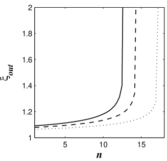
(a)

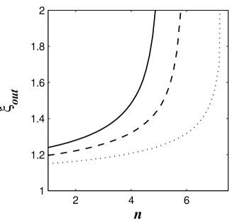
(b)

Figure 3: The curves of $\xi_{out}$ versus $n$ for the given values of $\theta_{M}$ with $\theta_{M}=0$ (solid line), $\pi/6$ (dashed line) and $\pi/4$ (dotted line); (a) $a_{*}=0$ , (b) $a_{*}=0.998$.

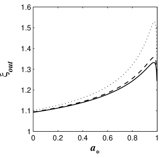
Figure 4: The curves of $\xi_{out}$ versus $a_{*}$ for $\theta_{M}=0$ and $0<a_{*}<0.998$ with $n=1.1$ (solid line), $n=1.5$ (dashed line), and $n=3$ (dotted line).

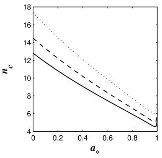
Figure 5: The curves of $n_{c}$ versus $a_{*}$ for the given values of $\theta_{M}$ with $\theta_{M}=0$ (solid line), $\pi/6$ (dashed line) and $\pi/4$ (dotted line).

4 COMPARISON OF POWER AND TORQUE IN THE BZ PROCESS AND MC PROCESS

In order to compare the relative strength of MC power to the BZ power and torque we define the ratio of $P_{MC}$ to $P_{BZ}^{optimal}$ and that of $T_{MC}$ to $T_{BZ}^{optimal}$ as follows,

$$\gamma \equiv {{P_{MC}}\mathord{\left/{\vphantom{{P_{MC}}{P_{BZ}^{optimal}}}}\right.\kern-1.2pt}{P_{BZ}^{optimal}}}$$ (35)

$$= \frac{{2a_{*}^{2}Q}}{{\left({arctanQ-{{a_{*}}\mathord{\left/{\vphantom{{a_{*}}2}}\right.\kern-1.2pt}2}}\right)}}\int_{\theta_{M}}^{{\pi\mathord{\left/{\vphantom{\pi 2}}\right.\kern-1.2pt}2}}{\frac{{\beta\left({1-\beta}\right)\sin^{3}\theta d\theta}}{{2-\left({1-q}\right)\sin^{2}\theta}}}$$

$$\tau \equiv {{T_{MC}}\mathord{\left/{\vphantom{{T_{MC}}{T_{BZ}^{optimal}}}}\right.\kern-1.2pt}{T_{BZ}^{optimal}}}$$ (36)

$$= \frac{{a_{*}^{2}Q}}{{\left({arc\tan Q-{{a_{*}}\mathord{\left/{\vphantom{{a_{*}}2}}\right.\kern-1.2pt}2}}\right)}}\int_{\theta_{M}}^{{\pi\mathord{\left/{\vphantom{\pi 2}}\right.\kern-1.2pt}2}}{\frac{{\left({1-\beta}\right)\sin^{3}\theta d\theta}}{{2-\left({1-q}\right)\sin^{2}\theta}}}$$

Setting $\theta_{M}=0$ in equations (35) and (36), we have the curves of $\gamma$ and $\tau$ versus $a_{*}$ for the given parameter $n$, and those versus $n$ for the given $a_{*}$ as shown in Fig.6 and Fig.7, respectively.

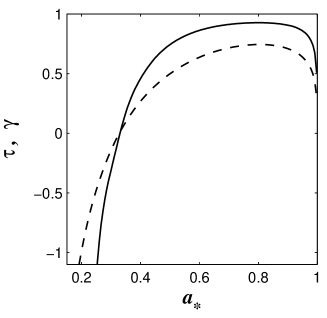
Figure 6: The curves of $\gamma$ (solid line) and $\tau$ (dashed line) versus the BH spin $a_{*}$ for $n=1.1$ and $0.2<a_{*}<0.998$.

Table 1: The three special values of $\gamma$ and the values of the concerning parameters

$n$	$\gamma=-1$	$\gamma=0$	$\gamma=\gamma_{max}$
$1.1$	$a_{*}^{\gamma 1}={\rm{0}}{\rm{.2583}}$	$a_{*}^{\gamma 2}={\rm{0}}{\rm{.3286}}$	$a_{*}^{\gamma m}=0.{\rm{7997}}$,
			$\gamma_{\max}=0.9278$
$1.5$	$a_{*}^{\gamma 1}={\rm{0}}{\rm{.2581}}$	$a_{*}^{\gamma 2}={\rm{0}}{\rm{.3283}}$	$a_{*}^{\gamma m}=0.{\rm{8002}}$,
			$\gamma_{\max}=0.9287$
$3.0$	$a_{*}^{\gamma 1}={\rm{0}}{\rm{.2572}}$	$a_{*}^{\gamma 2}={\rm{0}}{\rm{.3269}}$	$a_{*}^{\gamma m}=0.{\rm{8021}}$,
			$\gamma_{\max}=0.9325$

Table 2: The three special values of $\tau$ and the values of the concerning parameters

$n$	$\tau=-1$	$\tau=0$	$\tau=\tau_{max}$
$1.1$	$a_{*}^{\tau 1}={\rm{0}}{\rm{.1988}}$	$a_{*}^{\tau 2}={\rm{0}}{\rm{.3278}}$	$a_{*}^{\tau m}=0.{\rm{8045}}$,
			$\tau_{\max}=0.7452$
$1.5$	$a_{*}^{\tau 1}={\rm{0}}{\rm{.1987}}$	$a_{*}^{\tau 2}={\rm{0}}{\rm{.3275}}$	$a_{*}^{\tau m}=0.{\rm{8056}}$,
			$\tau_{\max}=0.7481$
$3.0$	$a_{*}^{\tau 1}={\rm{0}}{\rm{.1980}}$	$a_{*}^{\tau 2}={\rm{0}}{\rm{.3260}}$	$a_{*}^{\tau m}=0.{\rm{8118}}$,
			$\tau_{\max}=0.7614$

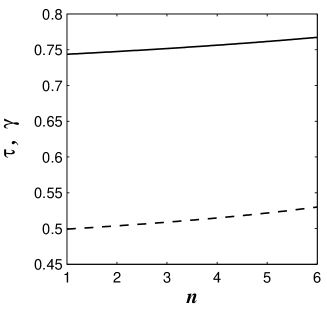
Figure 7: The curves of $\gamma$ (solid line) and $\tau$ (dashed line) versus the power-law index $n$ for $a_{*}=0.5$ and $1<n<6$.

The values of $a_{*}$ corresponding to the three special values of $\gamma$ ($\gamma=-1$, $0$ and $\gamma_{max}$) and to those of $\tau$($\tau=-1$, $0$ and $\tau_{max}$) are calculated for the given values of $n$ as shown in Table 1 and Table 2, respectively.

From the above calculations on $\gamma$ and $\tau$ we obtain the following results:
(i) The signs of $P_{MC}$ and $T_{MC}$ are the same as the corresponding $\gamma$ and $\tau$, and they change from the negative to the positive at $a_{*}^{\gamma 2}$ and $a_{*}^{\tau 2}$ respectively. It is shown in Table 1 and Table 2 that $a_{*}^{\tau 2}$ is a little less than $a_{*}^{\gamma 2}$. Therefore both energy and angular momentum are transferred from the BH to the disc as $a_{*}>a_{*}^{\gamma 2}$, and transferred from the disc to the BH as $a_{*}<a_{*}^{\tau 2}$. It is interesting to notice that the transfer direction of energy is opposite to that of angular momentum for $a_{*}^{\tau 2}<a_{*}<a_{*}^{\gamma 2}$, i.e., energy is transferred from the disc to the BH, while angular momentum from the BH to the disc in this value range of the BH spin.
(ii) Both $\gamma$ and $\tau$ vary non-monotonically as $a_{*}$ for the given parameter $n$, and attain their maxima at $a_{*}^{\gamma m}$ and $a_{*}^{\tau m}$, respectively;
(iii) The maxima of $P_{MC}$ and $T_{MC}$ are all less than the corresponding $P_{BZ}^{optimal}$ and $T_{BZ}^{optimal}$, respectively, while the absolute values of the former two are greater than the corresponding values of the latter two as $a_{*}$ is less than $a_{*}^{\gamma 1}$ and $a_{*}^{\tau 1}$, respectively.
(iv) As shown in Fig.7, both $\gamma$ and $\tau$ increase very little as the increasing parameter $n$, which implies that both $P_{MC}$ and $T_{MC}$ are insensitive to the power-law index $n$ of the radial coordinate $\xi$.

5 EVOLUTION CHARACTERISTICS AND ENERGY EXTRACTING EFFICIENCY

Based on conservation of energy and angular momentum the basic evolution equations of the Kerr BH in the coexistence of DABZMC are written as follows:

$${{dM}\mathord{\left/{\vphantom{{dM}{dt}}}\right.\kern-1.2pt}{dt}}=E_{ms}\dot{M}_{D}-P_{BZ}-P_{MC}$$ (37)

$${{dJ}\mathord{\left/{\vphantom{{dJ}{dt}}}\right.\kern-1.2pt}{dt}}=L_{ms}\dot{M}_{D}-T_{BZ}-T_{MC}$$ (38)

Incorporating equations (37) and (38), we have the evolution equation for the BH spin as follows:

$${{da_{*}}\mathord{\left/{\vphantom{{da_{*}}{dt}}}\right.\kern-1.2pt}{dt}} = M^{-2}\left({L_{ms}\dot{M}_{D}-T_{BZ}-T_{MC}}\right)$$ (39)

$$-2M^{-1}a_{*}\left({E_{ms}\dot{M}_{D}-P_{BZ}-P_{MC}}\right)$$

where $\dot{M}_{D}$ is the accretion rate of rest mass, $E_{ms}$ and $L_{ms}$ are specific energy and specific angular momentum corresponding to the inner edge radius $r_{ms}$, respectively.

Since the magnetic field on the BH is supported by the surrounding disc, there are some relations between $B_{H}$ and $\dot{M}_{D}$. As a matter of fact these relations might be rather complicated, and would be very different in different situations. One of them is given to investigate the correlation between BH spin and dichotomy of quasars by considering the balance between the pressure of the magnetic field on the horizon and the ram pressure of the innermost parts of an accretion flow (Moderski, Sikora & Lasota 1997), i.e.,

$$B_{H}^{2}/(8\pi)=P_{ram}\sim\rho c^{2}\sim\dot{M}_{D}/(4\pi r_{H}^{2})$$ (40)

From equation (40) we assume the relation as

$$\dot{M}_{D}={{B_{H}^{2}M^{2}\left({1+q}\right)^{2}}\mathord{\left/{\vphantom{{B_{H}^{2}M^{2}\left({1+q}\right)^{2}}2}}\right.\kern-1.2pt}2}$$ (41)

However equation (41) is derived without MC effects. By considering the transfer of the energy and angular momentum between the BH and the disc equations (41) is modified as follows:

$$\dot{M}_{D}={{B_{H}^{2}M^{2}\left({1+q}\right)^{2}}\mathord{\left/{\vphantom{{B_{H}^{2}M^{2}\left({1+q}\right)^{2}}2}}\right.\kern-1.2pt}2}+\left[{1-\delta\left({\theta_{M}-{\pi\mathord{\left/{\vphantom{\pi 2}}\right.\kern-1.2pt}2}}\right)}\right]\left({\dot{M}_{D}}\right)_{mc}$$ (42)

where $\left({\dot{M}_{D}}\right)_{mc}$ is the MC correction to the accretion rate at the inner edge of the disc, and it reads

$$\left(\dot{M}_{D}\right)_{mc}=$$ (43)

$$-\frac{{4B_{H}^{2}M^{2}Q\left({\chi_{ms}^{3}+a_{*}}\right)^{2}\left({1-\beta}\right)}}{{\left({\chi_{ms}^{3}+4a_{*}}\right)}}\sqrt{\frac{{1+a_{*}^{2}\chi_{ms}^{-4}+2a_{*}^{2}\chi_{ms}^{-6}}}{{1-2\chi_{ms}^{-2}+a_{*}^{2}\chi_{ms}^{-4}}}}$$

The derivation of equation (43) is given in Appendix A. To exclude $\left({\dot{M}_{D}}\right)_{mc}$ from the case without magnetic coupling we define $\delta\left({\theta_{M}-{\pi\mathord{\left/{\vphantom{\pi 2}}\right.\kern-1.2pt}2}}\right)$ as follows:

$$\delta(\theta_{M}-\pi/2)\equiv\left\{\begin{array}[]{r@{\quad\quad}l}1,&\theta_{M}=\pi/2,\\ 0,&0\leq\theta_{M}<\pi/2\end{array}\right.$$ (44)

Thus the equation (42) is applicable to the coexistence of DABZMC.
Setting $\dot{M}_{D}=0$ in equation (42), we can derive a value of the BH spin, $a_{*}^{stop}\approx 0.4677$, at which the accretion will stop at the inner edge of the disc. Substituting equation (42) into equations (37)$-$(39), we have

$${{dM}\mathord{\left/{\vphantom{{dM}{dt}}}\right.\kern-1.2pt}{dt}}=f\left({a_{*},u_{j}}\right)\dot{M}_{D}$$ (45)

$${{dJ}\mathord{\left/{\vphantom{{dJ}{dt}}}\right.\kern-1.2pt}{dt}}=Mh\left({a_{*},u_{j}}\right)\dot{M}_{D}$$ (46)

$${{da_{*}}\mathord{\left/{\vphantom{{da_{*}}{dt}}}\right.\kern-1.2pt}{dt}}=M^{-1}g\left({a_{*},u_{j}}\right)\dot{M}_{D}$$ (47)

where

$$g\left({a_{*},u_{j}}\right)=h\left({a_{*},u_{j}}\right)-2a_{*}f\left({a_{*},u_{j}}\right)$$ (48)

In the above equations $u_{j}\equiv\theta_{M},k,n$ is used for simplicity to represent the three parameters other than $a_{*}$. $f(a_{*},u_{j})$ and $g(a_{*},u_{j})$ are referred to as the characteristics functions (CFs) of BH evolution.

5.1 Evolution characteristics of Kerr BH

First we discuss the evolution characteristics of the Kerr BH in the coexistence of disc accretion with the BZ process for $\theta_{M}=\pi/2$. From equations (37)$-$(39) we have the CFs as follows:

$$f\left({a_{*},k}\right)=E_{ms}-{{P_{BZ}}\mathord{\left/{\vphantom{{P_{BZ}}{\dot{M}_{D}}}}\right.\kern-1.2pt}{\dot{M}_{D}}}$$ (49)

$$h\left({a_{*},k}\right)=M^{-1}\left({L_{ms}-{{T_{BZ}}\mathord{\left/{\vphantom{{T_{BZ}}{\dot{M}_{D}}}}\right.\kern-1.2pt}{\dot{M}_{D}}}}\right)$$ (50)

$$g\left({a_{*},k}\right)=h\left({a_{*},k}\right)-2a_{*}f\left({a_{*},k}\right)$$ (51)

From equations (45) and (47) we find that the signs of $dM/dt$ and $da_{*}/dt$ are the same as those of $f\left({a_{*},k}\right)$ and $g\left({a_{*},k}\right)$, respectively. As shown in Fig.8 we have the curve represented by $g\left({a_{*},k}\right)=0$ in the 2-dimension space consisting of the parameters $a_{*}$ and $k$, which divides the parameter space into two regions. And each black dot with arrowhead is referred to as a representative point (RP), which represents one BH evolution state. We can use RP’s displacement in the parameter space to describe BH evolution visually. According to the positions of RPs we have two evolution modes of the BH, and the details are given as follows.

(I) Region I: $f(a_{*},k)>0$ and $g(a_{*},k)<0$.
Mode I: RPs in Region I always move towards the left until they arrive at the boundary curve $g\left({a_{*},k}\right)=0$, i.e., BH will reach its equilibrium spin $a_{*}^{eq}$ in long enough evolution time. RPs in region I represent the BHs with increasing mass and decreasing spin.
(II) Region II: $f(a_{*},k)>0$ and $g(a_{*},k)>0$.
Mode II: RPs in Region II always move towards the right until they arrive at the boundary curve $g\left({a_{*},k}\right)=0$, i.e., BH will reach its equilibrium spin $a_{*}^{eq}$ in long enough evolution time. RPs in region II represent the BHs with increasing mass and increasing spin.
Next we shall discuss BH evolution in the coexistence of disc accretion with MC process. Substituting $\theta_{M}=0$ and equation (42) into equations (37)$-$(39), we have the corresponding CFs as follows:

$$f\left({a_{*},n}\right)=E_{ms}-{{P_{MC}}\mathord{\left/{\vphantom{{P_{MC}}{\dot{M}_{D}}}}\right.\kern-1.2pt}{\dot{M}_{D}}}$$ (52)

$$h\left({a_{*},n}\right)=M^{-1}\left({L_{ms}-{{T_{MC}}\mathord{\left/{\vphantom{{T_{MC}}{\dot{M}_{D}}}}\right.\kern-1.2pt}{\dot{M}_{D}}}}\right)$$ (53)

$$g\left({a_{*},n}\right)=h\left({a_{*},n}\right)-2a_{*}f\left({a_{*},n}\right)$$ (54)

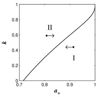
Figure 8: Parameter space for BH evolution in the BZ process with $0<k<1$ and $0.7<a_{*}<1$.

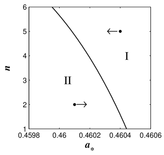
Figure 9: Parameter space for BH evolution in MC process with $1<n<6$ and $0.4598<a_{*}<0.4606$.

We can also describe BH evolution by using the displacement of RPs in 2-dimension parameter space consisting of the parameters $a_{*}$ and $n$ as shown in Fig.9, which is divided into two regions by the curve $g\left({a_{*},n}\right)=0$. In this case the description of the BH evolution characteristics and the two evolution modes are almost the same as that given in the BZ process except that $f\left({a_{*},k}\right)$ and $g\left({a_{*},k}\right)$ are replaced by $f\left({a_{*},n}\right)$ and $g\left({a_{*},n}\right)$, respectively. Inspecting Fig.8 and Fig.9, we have the following results:
(i) The CFs in the corresponding parameter space can be used to describe the evolution characteristics of the BH in a visual way. If we know the initial position of RP in the parameter space, we can determine the evolution characteristics of the BH immediately.
(ii) The effects of the parameter $k$ and $n$ on the BH evolution in the BZ and MC process can be easily found in the corresponding parameter space. From Fig.8 we find that $a_{*}^{eq}$ increases as the increasing $k$, which is consistent with our previous work (WLY). On the other hand, we find from Fig.9 that $a_{*}^{eq}$ increases very little as the decreasing $n$. Our calculations show that the values of $a_{*}^{eq}$ are very near to and a little less than $a_{*}^{stop}\approx 0.4677$.
(iii) As shown in Fig.5, the value range of $n$ is limited and confined by conservation of magnetic flux. Compared with the parameter $k$, the effects of $n$ on the variation of $a_{*}^{eq}$ are very weak for the confined value range of $n$.

5.2 Energy extracting efficiency of BH accretion disc

Energy extracting efficiency of BH accretion disc can be investigated also by using the CFs. From equations (45) and (47) we have

$${{dM}\mathord{\left/{\vphantom{{dM}M}}\right.\kern-1.2pt}M}=\left[{{{f\left({a_{*},u_{j}}\right)}\mathord{\left/{\vphantom{{f\left({a_{*},u_{j}}\right)}{g\left({a_{*},u_{j}}\right)}}}\right.\kern-1.2pt}{g\left({a_{*},u_{j}}\right)}}}\right]da_{*}$$ (55)

As is well known, a Kerr BH can be characterized by its mass $M$ and spin $a_{*}$. If a Kerr BH evolves from the initial state $(a_{*0},M_{0})$ to the state $(a_{*},M)$, the BH mass can be expressed by

$$M=M_{0}\exp\left[{\int_{a_{*0}}^{a_{*}}\frac{f(a_{*}^{{}^{\prime}},u_{j})}{g(a_{*}^{{}^{\prime}},u_{j})}}da_{*}^{{}^{\prime}}\right].$$ (56)

The efficiency corresponding to the evolution process of BH can be defined as

$$\eta_{p}=\frac{{M_{D}-\left({M-M_{0}}\right)}}{{M_{D}}}=1-\frac{{{M\mathord{\left/{\vphantom{M{M_{0}}}}\right.\kern-1.2pt}{M_{0}}}-1}}{{{{M_{D}}\mathord{\left/{\vphantom{{M_{D}}{M_{0}}}}\right.\kern-1.2pt}{M_{0}}}}}$$ (57)

which is the efficiency of converting accreted mass into radiation energy during the evolution process, and $M_{D}$ is the accreted rest mass and expressed as a function of $a_{*}$ by using equations (47) and (56) as follows:

$$M_{D}=M_{0}\int_{a_{*0}}^{a_{*}}{\frac{1}{{g\left({a_{*},u_{j}}\right)}}}\exp\left[{\int_{a_{*0}}^{a_{*}}{\frac{{f\left({a_{*}^{{}^{\prime}},u_{j}}\right)}}{{g\left({a_{*}^{{}^{\prime}},u_{j}}\right)}}da_{*}^{{}^{\prime}}}}\right]da_{*}$$ (58)

The efficiency corresponding to each evolving state of the BH is defined as

$$\eta_{s}=\frac{{dM_{D}-dM}}{{dM_{D}}}=1-{{\left({{{dM}\mathord{\left/{\vphantom{{dM}{dt}}}\right.\kern-1.2pt}{dt}}}\right)}\mathord{\left/{\vphantom{{\left({{{dM}\mathord{\left/{\vphantom{{dM}{dt}}}\right.\kern-1.2pt}{dt}}}\right)}{\dot{M}_{D}}}}\right.\kern-1.2pt}{\dot{M}_{D}}}=1-f\left({a_{*},u_{j}}\right)$$ (59)

From equation (37) we find that efficiency $\eta_{s}$ is equal to the sum of the following three terms:

$$\eta_{s}=\eta_{DA}+\eta_{BZ}+\eta_{MC}$$ (60)

where $\eta_{DA}=1-E_{ms}$, $\eta_{BZ}=P_{BZ}/\dot{M}_{D}$ and $\eta_{MC}=P_{MC}/\dot{M}_{D}$ are the contributions of disc accretion, the BZ process and MC process, respectively. From equation (47) we know that the equilibrium spin $a_{*}^{eq}$ is determined by

$$g\left({a_{*},u_{j}}\right)=0$$ (61)

Incorporating equations (55)$-$(59), we have

$$\left.{\eta_{p}}\right|_{a_{*}\to a_{*}^{eq}}=\mathop{\lim}\limits_{a_{*}\to a_{*}^{eq}}\left({1-{A\mathord{\left/{\vphantom{AB}}\right.\kern-1.2pt}B}}\right)$$ (62)

In equation (62) we have

$$A\equiv\exp\int_{a_{*0}}^{a_{*}}{\frac{{f\left({a_{*}^{{}^{\prime}},u_{j}}\right)}}{{g\left({a_{*}^{{}^{\prime}},u_{j}}\right)}}da_{*}^{{}^{\prime}}}-1\to\infty$$

and

$$B\equiv\int_{a_{*0}}^{a_{*}}{\frac{1}{{g\left({a_{*},u_{j}}\right)}}}\exp\left[{\int_{a_{*0}}^{a_{*}}{\frac{{f\left({a_{*}^{{}^{\prime}},u_{j}}\right)}}{{g\left({a_{*}^{{}^{\prime}},u_{j}}\right)}}da_{*}^{{}^{\prime}}}}\right]da_{*}\to\infty$$

By using L’ Hospital limit rule for $\infty/\infty$ type we have

$$\left.{\eta_{p}}\right|_{a_{*}\to a_{*}^{eq}}=1-f\left({a_{*}^{eq},u_{j}}\right)=\eta_{s}^{eq}\left({a_{*}^{eq},u_{j}}\right)$$ (63)

where $\eta_{s}^{eq}$ represents the efficiency $\eta_{s}$ at $a_{*}^{eq}$. Equation (63) implies that the efficiency $\eta_{p}$ is exactly equal to $\eta_{s}^{eq}$, provided that a BH evolves from any spin $a_{*0}$ to its equilibrium spin $a_{*}^{eq}$. Incorporating equations (42), (59), (61) and (37)$-$(39), we obtain the curves of $a_{*}^{eq}$ and $\eta_{s}^{eq}$ varying as the concerning parameters are shown in Fig.10.

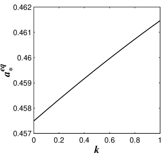
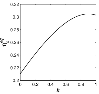
(a)  (d)

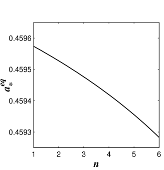
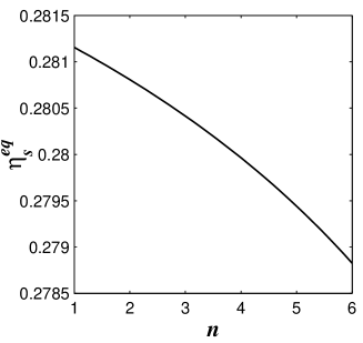
(b)  (e)

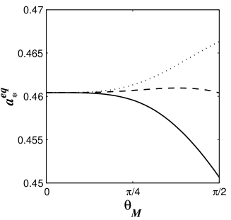
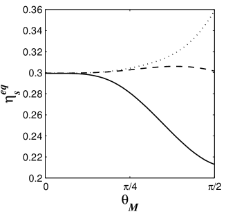
(c)  (f)

Figure 10: The curves of $a_{*}^{eq}$ and $\eta_{s}^{eq}$ varying as the concerning parameters. (a), (d) $\theta_{M}=\pi/4$, $0<k<1$, $n=1.1$; (b), (e) $\theta_{M}=\pi/4$, $k=0.5$, $1<n<6$; (c), (f) $0<\theta_{M}<\pi/2$, $n=1.1$, $k=0.5$(solid line), $k=0.788$(dashed line); $k=0.96$(dotted line).

Comparing Fig.10a, b, c with Fig.10d, e, f we find the following results:

(i) The curves of $a_{*}^{eq}$ and $\eta_{s}^{eq}$ varying as the concerning parameters look very alike except that $\eta_{s}^{eq}$ varies as $k$ non-monotonically with its maximum $(\eta_{s}^{eq})_{max}\approx 30.5\%$ at $a_{*}^{eq}\approx 0.4611$ for $k\approx 0.8998$ as shown in Fig.10d.

(ii) Both $a_{*}^{eq}$ and $\eta_{s}^{eq}$ decrease monotonically as the increasing $n$ for $\theta_{M}=\pi/4$ as shown in Fig.10b and Fig.10e. Considering that the outer boundary $\xi_{out}$ increase monotonically as the increasing $n$, we infer that the more concentrated is the magnetic field on the central region of the disc, the wider is the MC region on the disc, the stronger is the braking effects of MC process on the BH spin, and the lower are the $a_{*}^{eq}$ and $\eta_{s}^{eq}$.

(iii) As shown in Figs.10c and 10f the variations of $a_{*}^{eq}$ and $\eta_{s}^{eq}$ as $\theta_{M}$ display different characteristics for different values of parameter $k$: They might increase as $\theta_{M}$ (dotted line) or decreases as $\theta_{M}$ (solid line) or almost remain unchanged with $\theta_{M}$ (dashed line). It is not difficult to understand these results by considering that $\theta_{M}$ is the angular boundary between the open and closed field lines on the BH horizon: The different variations of $a_{*}^{eq}$ and $\eta_{s}^{eq}$ as $\theta_{M}$ come from the different contributions due to the BZ and MC process. For example, $a_{*}^{eq}$ and $\eta_{s}^{eq}$ will increase as $\theta_{M}$ , if the contributions of the open field lines in unit angular coordinate are greater than those corresponding to the closed ones, while they will decrease as $\theta_{M}$ in case that the former is less than the latter.

In summary we can calculate the efficiency in an evolution process and that corresponding to each evolving state of the Kerr BH by using the equations (57) and (59), respectively, and both of which are expressed in terms of the CFs.

6 BH ENTROPY CHANGE IN COEXISTENCE OF DABZMC

It was shown that the excess rate of change of entropy of the central BH in the BZ process comes from the total power dissipation on the BH horizon (WLY). It is attractive for us to extend this result to the coexistence of DABZMC. As is well known, the BH temperature $T_{H}$ and entropy $S_{H}$ can be expressed as (Thorne, Price & Macdonald 1986, hereafter TPM)

$$T_{H}=\frac{q}{{4\pi M(1+q)}},S_{H}=2\pi M^{2}(1+q)$$ (64)

Incorporating the basic evolution equations (37), (38) and (39), we have the following equations,

$$\begin{array}[]{l}T_{H}{{dS_{H}}/{dt}}={{dM}/{dt}}-\Omega_{H}{{dJ}/{dt}}=(E_{ms}-\\ \Omega_{H}L_{ms})\dot{M}_{D}+\left({\Omega_{H}T_{BZ}-P_{BZ}}\right)+\left({\Omega_{H}T_{MC}-P_{MC}}\right)\\ \end{array}$$ (65)

equation (65) is exactly the mathematical formulation of the first law of thermodynamics for a Kerr BH (TPM). Obviously, the first term on RHS of equation (65) is the contribution due to disc accretion. It is easy to prove that the second and the third term arise from power dissipation on the BH horizon due to the BZ and MC process, respectively. By using the improved equivalent circuit as shown in Fig.2 and equation (11) we have

$$I\Delta\varepsilon_{H}=I^{2}\Delta Z_{H}+I^{2}\Delta Z_{L}-I\Delta\varepsilon_{L}$$ (66)

Incorporating equations (9), (11), (13) and $\Delta\varepsilon_{L}=-\left({{{\Delta\Psi}\mathord{\left/{\vphantom{{\Delta\Psi}{2\pi}}}\right.\kern-1.2pt}{2\pi}}}\right)\Omega_{L}$ we obtain

$$\Delta P=\left({{{\Delta\Psi}\mathord{\left/{\vphantom{{\Delta\Psi}{2\pi}}}\right.\kern-1.2pt}{2\pi}}}\right)^{2}\frac{{\Omega_{F}\left({\Omega_{H}-\Omega_{F}}\right)}}{{\Delta Z_{H}}}=I^{2}\Delta Z_{L}-I\Delta\varepsilon_{L}$$ (67)

From equations (66) and (67) we find that $I\Delta\varepsilon_{H}$ consists of two parts: the extracting power $\Delta P$ and the dissipated power $\Delta P_{DSP}$. The extracting power is transferred to the load including both the remote astrophysical load and the load disc. For the BZ process $\Delta\varepsilon_{L}=0$, we have

$$\Delta P=\Delta P_{BZ}=I^{2}\Delta Z_{L}=\left({{{\Delta\Psi}\mathord{\left/{\vphantom{{\Delta\Psi}{2\pi}}}\right.\kern-1.2pt}{2\pi}}}\right)^{2}\frac{{\Omega_{F}\left({\Omega_{H}-\Omega_{F}}\right)}}{{\Delta Z_{H}}}$$ (68)

For MC process $\Delta Z_{L}=0$, we have

$$\Delta P=\Delta P_{MC}=-I\Delta\varepsilon_{L}=\left({{{\Delta\Psi}\mathord{\left/{\vphantom{{\Delta\Psi}{2\pi}}}\right.\kern-1.2pt}{2\pi}}}\right)^{2}\frac{{\Omega_{D}\left({\Omega_{H}-\Omega_{D}}\right)}}{{\Delta Z_{H}}}$$ (69)

Incorporating equations (11), (12) and (13), we can express the dissipated power $\Delta P_{DSP}$ on the BH horizon as

$$\Delta P_{DSP}=I^{2}\Delta Z_{H}={{\left({{{\Delta\Psi}\mathord{\left/{\vphantom{{\Delta\Psi}{2\pi}}}\right.\kern-1.2pt}{2\pi}}}\right)^{2}\left({\Omega_{H}-\Omega_{F}}\right)^{2}}\mathord{\left/{\vphantom{{\left({{{\Delta\Psi}\mathord{\left/{\vphantom{{\Delta\Psi}{2\pi}}}\right.\kern-1.2pt}{2\pi}}}\right)^{2}\left({\Omega_{H}-\Omega_{F}}\right)^{2}}{\Delta Z_{H}}}}\right.\kern-1.2pt}{\Delta Z_{H}}}$$

$$=\Omega_{H}\Delta T-\Delta P$$ (70)

Integrating equation (70) over the angular coordinate $\theta$, we obtain the total dissipated power on the horizon, which is exactly equal to the sum of the second and the third term on RHS of equation (65), i.e.,

$$P_{DSP}=\left({P_{DSP}}\right)_{BZ}+\left({P_{DSP}}\right)_{MC}$$ (71)

where $\left({P_{DSP}}\right)_{BZ}=\left({\Omega_{H}T_{BZ}-P_{BZ}}\right)$ and $\left({P_{DSP}}\right)_{MC}=\left({\Omega_{H}T_{MC}-P_{MC}}\right)$ are the total power dissipation due to the BZ and MC process, respectively. Combining equations (15), (16), (20) and (21) we have

$$\left({P_{DSP}}\right)_{BZ} = \Omega_{H}T_{BZ}-P_{BZ}$$ (72)

$$= 2a_{*}^{2}B_{H}^{2}M^{2}\int_{0}^{\theta_{M}}{\frac{{\left({1-k}\right)^{2}\sin^{3}\theta d\theta}}{{2-\left({1-q}\right)\sin^{2}\theta}}}$$

$$\left({P_{DSP}}\right)_{MC} = \Omega_{H}T_{MC}-P_{MC}$$ (73)

$$= 2a_{*}^{2}B_{H}^{2}M^{2}\int_{\theta_{M}}^{{\pi\mathord{\left/{\vphantom{\pi 2}}\right.\kern-1.2pt}2}}{\frac{{\left({1-\beta}\right)^{2}\sin^{3}\theta d\theta}}{{2-\left({1-q}\right)\sin^{2}\theta}}}$$

Incorporating equations (65), (72) and (73), we express the rates of change of BH entropy corresponding to disc accretion, the BZ and MC process as follows:

$$\left({{{dS_{H}}\mathord{\left/{\vphantom{{dS_{H}}{dt}}}\right.\kern-1.2pt}{dt}}}\right)_{DA}=T_{H}^{-1}\left({E_{ms}-\Omega_{H}L_{ms}}\right)\dot{M}_{D}$$ (74)

$$\left({{{dS_{H}}\mathord{\left/{\vphantom{{dS_{H}}{dt}}}\right.\kern-1.2pt}{dt}}}\right)_{BZ}=T_{H}^{-1}\left({\Omega_{H}T_{BZ}-P_{BZ}}\right)$$ (75)

$$\left({{{dS_{H}}\mathord{\left/{\vphantom{{dS_{H}}{dt}}}\right.\kern-1.2pt}{dt}}}\right)_{MC}=T_{H}^{-1}\left({\Omega_{H}T_{MC}-P_{MC}}\right)$$ (76)

From the above analysis we conclude that the excess rate of change of the BH entropy does come from the total power dissipation on the BH horizon in the BZ and MC process.

The ratios of the rates of BH entropy change can be written by

$$R_{BZDA}\left({a_{*},\theta_{M},k}\right)=\frac{({{dS_{H}}/{dt}})_{BZ}}{({{dS_{H}}/{dt}})_{DA}}$$

$$=\frac{{\Omega_{H}T_{BZ}-P_{BZ}}}{{\left({E_{ms}-\Omega_{H}L_{ms}}\right)\dot{M}_{D}}}$$ (77)

$$R_{MCDA}\left({a_{*},\theta_{M},n}\right)=\frac{{\left({{{dS_{H}}\mathord{\left/{\vphantom{{dS_{H}}{dt}}}\right.\kern-1.2pt}{dt}}}\right)_{MC}}}{{\left({{{dS_{H}}\mathord{\left/{\vphantom{{dS_{H}}{dt}}}\right.\kern-1.2pt}{dt}}}\right)_{DA}}}$$

$$=\frac{{\Omega_{H}T_{MC}-P_{MC}}}{{\left({E_{ms}-\Omega_{H}L_{ms}}\right)\dot{M}_{D}}}$$ (78)

where the four parameters $k$, $a_{*}$, $\theta_{M}$ and $n$ are involved. Letting one of them vary and the rest be fixed, we have the curves of $R_{BZDA}$ and $R_{MCDA}$ versus $a_{*}$ and $\theta_{M}$ as shown in Fig.11, and the following results are obtained:

(i) As shown in Figs.11a and 11b $R_{BZDA}$ increases monotonically as $a_{*}$ for the given values of $k$ and $\theta_{M}$, while $R_{MCDA}$ varies non-monotonically and attains a minimum approach zero at $a_{*}\approx{\rm{0}}{\rm{.3305}}$ for the given values of $n$ and $\theta_{M}$. From the discussion in Sec.IV we know that the minimum of $R_{MCDA}$ arises from the neighboring $a_{*}^{\gamma 2}$ and $a_{*}^{\tau 2}$ corresponding to $P_{MC}=0$ and $T_{MC}=0$, respectively.

(ii) As shown in Figs.11a and 11b we have $R_{MCDA}>R_{BZDA}$ for $0<a_{*}<0.2694$ and $0.4373<a_{*}<a_{*}^{eq}$, which implies that the contribution to $P_{DSP}$ and BH entropy increase due to MC process dominates over that due to the BZ process in the above value range of the BH spin.

(iii) As shown in Fig.11c the ratio $R_{BZDA}$ increases monotonically as $\theta_{M}$ for the given values of $a_{*}$ and $k$, while $R_{MCDA}$ varies non-monotonically as $\theta_{M}$ for the above given values of $a_{*}$ and $n$. $R_{MCDA}$ is greater than $R_{BZDA}$ for $0<\theta_{M}<0.{\rm{6782}}$, while the former is much less than the latter for $0.6782<\theta_{M}<{\pi\mathord{\left/{\vphantom{\pi 2}}\right.\kern-1.2pt}2}$. It is obvious that the sum of the two is much less than unity, which implies that the contribution to BH entropy increase is dominated by disc accretion in the coexistence of DABZMC.

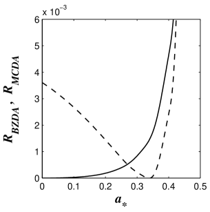
(a)

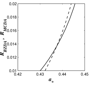
(b)

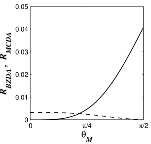
(c)

Figure 11: The curves of $R_{BZDA}$ (solid line) and $R_{MCDA}$(dashed line) versus the concerning parameters, (a), (b) $0<a_{*}<1$, $\theta_{M}=\pi/4$, $k=0.5$, $n=1.1$; (c) $0<\theta_{M}<\pi/2$, $a_{*}=0.4$, $k=0.5$, $n=1.1$.

7 SUMMARY

In this paper the evolution characteristics of a Kerr BH and some related issues, such as energy extracting efficiency and entropy change on the BH horizon, are investigated by considering coexistence of DABZMC. By using an improved equivalent circuit a unified expression for the BZ power and MC power are derived. Starting from the conservation laws of energy and angular momentum, we obtain the basic evolution equations of the BH and the CFs in terms of four parameters related to our model, i.e., $a_{*}$, $\theta_{M}$, $k$ and $n$. We find that the evolution characteristics of the Kerr BH can be well described by using the CHs and the RPs in the corresponding parameter space.

It turns out that the main difference between the BZ process and MC process lies in the two kinds of loads: the remote load with an unknown parameter $k$ for the BZ process, and the load disc with the parameter $\beta$ for MC process. Parameter $k$ is uncertain, while $\beta$ is thoroughly determined by the BH spin and the place where the magnetic flux penetrates. The effects of MC process on the evolution of the BH and the efficiency of BH accretion disc can be discussed in virtue of the parameters $a_{*}$, $\theta_{M}$ and $n$, into which the parameter $\beta$ is merged.

In this model the mapping relation between the BH horizon and the disc is derived by assuming a power-law of the magnetic field varying as the radial coordinate of the disc. It is shown that the power-law index $n$ is related to the outer boundary parameter $\xi_{out}$. And the MC correction to the accretion rate is considered by using the conservation law of angular momentum. Only the accretion rate at the inner edge of the disc being involved in the evolution equations of the BH, the correction to the accretion rate is made by taking the corresponding values at $r_{ms}$ in our simplified model.

In summary this model provides an analytic approach to the evolution characteristics and related physical quantities of a Kerr black hole surrounded by magnetized accretion disc.

ACKNOWLEDGEMENTS
This work is supported by the National Natural Science Foundation of China under Grant No. 10173004. We are very grateful to the anonymous referee for his suggestions about the MC effects on the accretion rate and the constraints to the parameters of MC process.

Appendix A Derivation of equation(43)

In the case without magnetic coupling between the BH and the disc, accretion is produced by the internal viscous torque $T_{vis}$ of the disc. By using the conservation law of angular momentum the accretion rate $\dot{M}_{D}$ is related to $T_{vis}$ by the following equation (Frank, King & Raine 1992):

$$-\dot{M}_{D}\partial(r^{2}\Omega_{D})/\partial r=\partial T_{vis}/\partial r$$ (79)

where $\partial T_{vis}/\partial r$ is the contribution due to internal viscous torque, always transporting angular momentum outward in the disc. Taking MC effects into account, we think equation (A1) should be modified by

$$-\dot{M}_{D}\partial(r^{2}\Omega_{D})/\partial r=\partial T_{vis}/\partial r-\partial T_{MC}/\partial r$$ (80)

where $\partial T_{MC}/\partial r$ is the contribution due to MC torque, and the minus sign arises from the consideration that the contribution of $\partial T_{vis}/\partial r$ should be counteracted by $\partial T_{MC}/\partial r$ in case $\Omega_{D}<\Omega_{H}$. Comparing equations (A1) and (A2), we express $(\dot{M}_{D})_{mc}$, the contribution of MC effects to the accretion rate, as follows:

$$(\dot{M}_{D})_{mc}=\frac{\partial T_{MC}}{\partial(r^{2}\Omega_{D})}=\frac{\partial T_{MC}/\partial r}{\partial(r^{2}\Omega_{D})/\partial r}$$ (81)

Substituting equations (6), (10), (12), (14) and (34) into equation (A3), we have

$$(\dot{M}_{D})_{mc} = \frac{4{B^{2}}_{H}M^{3}a_{*}(1+q)(1-\beta)\sin^{2}\theta}{2-(1-q)\sin^{2}\theta}$$ (82)

$$\times\frac{2(\chi^{3}+a_{*})^{2}}{r_{ms}\chi^{2}(\chi^{3}+4a_{*})}G(a_{*};\xi,n)$$

From equation (A4) we find that the MC correction depends on the place on the disc where the MC torque acts. Substituting the boundary values such as $\xi=\xi_{in}=1$ (i.e.,$r=r_{ms}=M\chi^{2}_{ms}$) and $\theta=\pi/2$ into equation (A4) we obtain equation (43), which is the MC correction to the accretion rate at the inner edge of the disc. In derivation the factor 2 is given for the two faces of the disc, and $B^{2}_{H}$ is also taken as the average value over the BH horizon.

References

- [1] Bardeen J. M., Press W. H., and Teukolsky S. A., 1972, ApJ, 178, 347
- [2] Blandford R. D., 1976, MNRAS, 176, 465
- [3] Blandford R. D., Znajek R. L., 1977, MNRAS, 179, 433
- [4] Blandford R. D., 1999 in Astrophysical Discs: An EC Summer School, Astronomical Society of the Pacific Confrence Series, ed. Scllwood J A & Goodman J 160, 265. 1999 preprint astro-ph/9902001
- [5] Frank J., King A. R., Raine D. L., 1985, Accretion Power in Astrophysics, Cambridge Univ. Press, Cambridge
- [6] Ghosh P., Abramowicz M. A., 1997, MNRAS 292, 887
- [7] Lee H. K., Wijers R. A. M. J., Brown G. E., 2000, Phys. Rep., 325, 83 (LWB) preprint astro-ph/9906213
- [8] Li L. -X. 2000a, ApJ, 533, 115L.
- [9] Li L. -X. 2000b, preprint astro-ph/0012469
- [10] Li L. -X., Paczynski B., 2000, ApJ, 534, 197L
- [11] Lu Y. J., Zhou Y. Y., Yu K. N., Young, E. C. M., 1996, ApJ, 472, 564
- [12] Macdonald D., Thorne K. S., 1982, MNRAS, 198, 345 (MT82)
- [13] Moderski R., Sikora M., 1996, MNRAS, 283, 854
- [14] Moderski R., Sikora M., Lasota J.P., 1997, in ”Relativistic Jets in AGNs” eds.M. Ostrowski, M. Sikora, G. Madejski & M. Belgelman, Krakow 1997, 110, preprint astro-ph/9706263
- [15] Park S. J., Vishniac E. T., 1988, ApJ, 332, 135
- [16] Punsly B., Coroniti F. V., 1990, ApJ, 350, 518
- [17] Rees M. J., 1984, ARA&A. 22, 471
- [18] Shapiro S. L., Teukolsky S. A., 1983, Black Holes, White Dwarfs and Neutron Stars , John Wiley & Sons, Inc. New York
- [19] Thorne K. S., Price R. H., Macdonald D. A., 1986, Black Holes: The Membrane Paradigm , Yale Univ. Press, New Haven and London (TPM)
- [20] Wang D. X., Lu Y., Yang L. T., 1998, MNRAS, 294, 667 (WLY)