Unbiased cut selection for optimal upper limits in neutrino detectors: the model rejection potential technique

Abstract

We present a method for optimising experimental cuts in order to place the strongest constraints (upper limits) on theoretical signal models. The method relies only on signal and background expectations derived from Monte-Carlo simulations, so no bias is introduced by looking at actual data, for instance by setting a limit based on expected signal above the “last remaining data event.” After discussing the concept of the “average upper limit,” based on the expectation from an ensemble of repeated experiments with no true signal, we show how the best model rejection potential is achieved by optimising the cuts to minimise the ratio of this “average upper limit” to the expected signal from the model. As an example, we use this technique to determine the limit sensitivity of kilometre scale neutrino detectors to extra-terrestrial neutrino fluxes from a variety of models, e.g. active galaxies and gamma-ray bursts. We suggest that these model rejection potential optimised limits be used as a standard method of comparing the sensitivity of proposed neutrino detectors.

and

1 Introduction

In this paper, we examine the problem of choosing experimental cuts in order to place the most restrictive limits on theoretical signal models. How should one choose cuts with this in mind? If a signal is assumed, the goal is to maximise the significance of the observation, by for instance optimising signal to noise or signal to square root noise. If, however, one assumes that no signal will be observed, a different technique is required to optimise the “model rejection potential,” i.e. the limit setting potential of an experiment. This technique must not depend on the experimental data, since choosing cuts based on the data (e.g. cutting after the last remaining event) leads to confidence intervals that do not have frequentist coverage.

In this paper, we describe and assess an unbiased method [1, 2], based only on Monte Carlo signal and background expectations.

Firstly we discuss how an experimental observation is used to set a limit on a theoretical flux (section 2). The desire to minimise the upper limit (and thus place the strongest constraint on the theoretical model) leads to the concepts of “average upper limits” and “model rejection factor,” which are discussed in section 3. We show how choosing cuts based on optimising the “model rejection factor” leads to, on average, the best possible limit from the experiment. In section 4, we illustrate this technique by calculating the model rejection potential of a kilometre scale neutrino detector with respect to predicted extra-terrestial neutrino fluxes such as active galaxies and gamma-ray bursts.

2 Calculating flux limits

When an experiment fails to detect an expected flux, an upper limit on that flux can be derived from the experimental observation. As an example consider a detector that should observe 100 signal events above an expected background of a few events. If only the few events consistent with background are observed, then obviously the model is strongly constrained as the 100 expected events were not seen. The exact calculation of an upper limit on the source flux would proceed as follows. The theoretical source flux, $\Phi(E,\theta)$, is convolved with the detector response and after some cuts yields an event expectation, $n_{s}$. Let the expected background for the same analysis and cuts be $n_{b}$. The experiment is performed and $n_{\mathit{obs}}$ events are seen.

In this experiment the 90% confidence interval $\mu_{90}=(\mu_{1},\mu_{2})$ is a function of the number of observed events, $n_{\mathit{obs}}$, and of the expected background $n_{b}$

$$\mu_{90}(n_{\mathit{obs}},n_{b})$$ (1)

For example, an experiment that observes 3 events on an expected background of 1.5 would report a $90\%$ confidence interval in the Feldman-Cousins [4] “unified” approach of $\mu_{90}(3,1.5)=(0.0,5.92)$. Note that this confidence interval includes 0.0, and therefore $\mu_{2}=5.92$ is an upper limit. In what follows we shall take $\mu_{90}$ to mean this upper limit.

The corresponding upper limit on the source spectrum $\Phi(E,\theta)$ is found by scaling the source flux by the ratio of the upper limit to the signal expectation [7]

$$\Phi(E,\theta)_{90\%}=\Phi(E,\theta)\frac{\mu_{90}(n_{\mathit{obs}},n_{b})}{n_{s}}$$ (2)

If the expected signal contribution to the observation was $n_{s}=100$, then the $90\%$ confidence level upper limit on the source flux is

$$\Phi(E,\theta)_{90\%}=\Phi(E,\theta)\times\frac{5.92}{100}$$ (3)

In this case the theoretical model predicts a large number of events with very few seen and is therefore severely constrained by the experiment. A low value of the ratio $\mu_{90}(n_{\mathit{obs}},n_{b})$/$n_{s}$ has led to a strong constaint on the model, therefore one should optimise cuts to make this ratio small. However, the observed upper limit depends on $n_{\mathit{obs}}$ which is not known until the cuts are defined and the experiment performed! Fortunately, the classical concept of an ensemble of experiments allows us to calculate an “average upper limit” (equivalent to the Feldman-Cousins “sensitivity” [4]) which can take the place of $\mu_{90}(n_{\mathit{obs}},n_{b})$ in the signal to upper limit calculation.

3 Average upper limits and “model rejection factor”

Although we cannot know the actual upper limit that will result from an experiment until looking at the data, we can use the Monte Carlo predictions to calculate the average upper limit (Feldman-Cousins “sensitivity” [4]) that would be observed after hypothetical repetition of the experiment with expected background $n_{b}$ and no true signal ($n_{s}=0$). In the example of the previous section, the expected background was $n_{b}=1.5$. Over an ensemble of experiments with no true signal, this background will fluctuate to $n_{\mathit{obs}}=0$ with Poisson probability 22.3% and an upper limit of $\mu_{90}(0,1.5)=1.33$ reported. The background will fluctuate to $n_{\mathit{obs}}=1$ in 33.5% of experiments, where an upper limit of 2.91 would be reported, and so on for each value of $n_{\mathit{obs}}$. The “average upper limit” is the sum of these expected upper limits, weighted by their Poisson probability of occurrence

$${\bar{{\mu}}_{90}(n_{b})}=\sum_{n_{\mathit{obs}}=0}^{\infty}\mu_{90}(n_{\mathit{obs}},n_{b})\;\;\frac{(n_{b})^{n_{\mathit{obs}}}}{(n_{\mathit{obs}})!}\exp(-n_{b})$$ (4)

This average upper limit is shown in figure 1 as a function of the expected background for four different Poisson confidence levels under the Feldman-Cousins “unified” ordering principle. Before performing the experiment, one can see what background would be expected to remain as a function of various cuts, then consult this plot to find out what average upper limit result the experiment would be expected to give.

Figure 1: Average 90% Feldman-Cousins upper limit that would be obtained by an ensemble of experiments with no true signal in the presence of expected background.

Over an ensemble of identical experiments, the strongest constraint on the expected signal flux $\Phi(E,\theta)$ corresponds to the set of cuts that minimises the “model rejection factor”

$$\frac{\bar{\mu}_{90}}{n_{s}}$$ (5)

and hence minimises the average flux upper limit that would be obtained over the hypothetical experimental ensemble

$$\bar{\Phi}(E,\theta)_{90}=\Phi(E,\theta)\frac{\bar{\mu}_{90}}{n_{s}}$$ (6)

In the actual experiment we will not obtain $\bar{\Phi}(E,\theta)_{90}$, but obtain one limit based on the observed number of background counts, which depends on how the background happened to fluctuate in the single, real experiment. However, prior to performing the experiment, the average flux upper limit (flux times model rejection factor) tells us what we would expect over repeated runs of the real experiment, and on average the best limit will come from choosing cuts that minimise this average limit. Also, the model rejection factor curve tells us how sensitive the expected limit is to the choice of cuts.

A somewhat common practice is to choose the final cut based on the last observed data event. The event limit $\mu_{90}$ then comes from the observation of zero events above that cut. This event limit is then compared to the predicted signal from the source flux above the cut, and the flux limit obtained using equation 2. Calculating the event limit in this way results in confidence intervals which do not have frequentist coverage. The classical concept of frequentist coverage [3, 4, 5] involves the construction of $(100\times\alpha)\%$ confidence intervals, such that in $(100\times\alpha)\%$ of repeated experiments, the reported confidence interval will include (“cover”) the fixed but unknown true value of the estimated parameter $\mu_{t}$. This coverage applies to any value that $\mu_{t}$ may take. Choosing the cut based on the last observed data event will lead to intervals that do not cover all possible values of $\mu_{t}$ with the correct frequency, as can be seen by a simple example. Assume that we are using a standard Neyman construction for a Poissonian upper limit. As a example, the 90% confidence level upper limit for zero observed events is $\mu=2.3$. If we always choose the cut such that zero events are observed, then we will always report an upper limit $\mu=2.3$. Thus, in any experiments where the true value of the parameter $\mu$ is greater than 2.3, the reported confidence interval, (always $\mu<2.3$), never covers the true value! At the other extreme, for true values $\mu_{t}<2.3$, the reported confidence interval will cover the true value in exactly $100\%$ of cases. In neither case is the required 90% coverage achieved, showing that choosing the final cut based on the observed data is not a valid method in the frequentist framework.

These considerations show that the final experimental cuts must be chosen prior to looking at the data, and that the model rejection potential technique provides a method of optimising these cuts to give the best average limit. In the next section we apply the model rejection potential technique to the determination of the sensitivity of proposed kilometre scale neutrino detectors to astrophysical sources of neutrinos, using searches for both diffuse and point like emissions as examples.

4 Model rejection potential of kilometre scale neutrino detectors

Various proposals exist for the construction of kilometre scale neutrino detectors [6] in the the deep ocean (the ANTARES, NESTOR and NEMO experiments) or in Antarctic ice (the Icecube experiment). These experiments look for upward moving muons which result from neutrino interactions in the surrounding media (water, ice or rock). The upgoing requirement is necessary to reject the large background flux of downgoing cosmic ray induced muons. After rejecting all downward events, the flux of atmospheric neutrinos from cosmic ray interactions in the earth’s atmosphere remains as the background to a search for extra-terrestrial neutrinos.

We can determine the sensitivity of an experiment to a flux of extra-terrestrial neutrinos by optimising the model rejection potential to find the average limit that would be placed on that flux if no true signal were present, and only the expected background atmospheric neutrino events observed. In the following sections, we use the searches for diffuse fluxes and point sources of extra-terrestrial neutrinos to illustrate the model rejection potential technique. For the diffuse flux case, the model rejection potential optimisation is done in one cut dimension, whereas in the point source case, we show how a two-dimensional optimisation is made. The method could in principle be generalised to an optimisation in $n$ dimensions, where the point in the $n$-dimensional cut parameter space is found where the model rejection factor is minimised.

Predicting the rate of upward moving neutrino induced muons in the vicinity of an underwater or underice detector is straightforward [8, 9, 10, 11, 12, 13, 14, 15, 16] and so we describe here only the basic elements of the calculation. The current calculation follows a previously described method [13, 14], where the neutrino cross sections are calculated using the “G” parton distribution set of Martin, Roberts and Stirling [17], the Lipari-Stanev [18] muon propagation code is used to track the muons to the detector, and the structure of the earth is accounted for using the Preliminary Reference Earth Model [19]. An important difference between this and other work is the exact treatment of neutral current regeneration of neutrinos in the earth using a recursive importance sampling interaction algorithm [13, 14]. Neutrino and anti-neutrino events were generated using an $E^{-1}$ spectrum, and then re-weighted to various astrophysical flux predictions. A constant detector muon effective area of $1\rm{km}^{2}$ was assumed for all angles and energies.

4.1 Model rejection potential optimisation for diffuse flux searches

We consider three types of diffuse neutrino flux predictions, firstly $E^{-2}$ spectra, an example of which is the Waxman-Bahcall diffuse upper bound [21] on the flux of astrophysical neutrinos. They calculate that the diffuse flux of neutrinos should not exceed a level

$$E^{2}\Phi_{\mathrm{WBUB}}=3.0\times 10^{-8}\;\mathrm{GeV}\;\mathrm{cm}^{-2}\;\mathrm{s}^{-1}\;\mathrm{sr}^{-1}$$ (7)

Mannheim, Protheroe and Rachen [22] question the assumptions made in the Waxman-Bahcall upper bound calculation and have computed fluxes of diffuse neutrinos that violate this upper bound. One of the Mannheim, Protheroe and Rachen models is also tested here. Finally, we determine the sensitivity of a kilometre scale detector to the original Stecker, Done, Salamon and Sommers [23] diffuse neutrino flux prediction. The atmospheric neutrino background to these searches is taken from the calculation of Lipari [24]. In calculating this background, we have not considered the uncertain contribution from the prompt charm decay channel [25, 26]. Including this neutrino flux in a background estimate requires incorporating the systematics into the limit calculation[27, 28]). Or, one could consider this flux as a source on which limits can be placed, though difficult to separate from an extra-terrestrial source [14].

We consider in detail the optimisation of the model rejection potential for a diffuse $E^{-2}$ source of astrophysical neutrinos. We will assume that the muon energy at the detector can be measured, and use this as the cut against the atmospheric neutrino induced background events. Figure  2 shows the differential energy distributions for the atmospheric neutrino-induced muons, and for the muons resulting from a diffuse $E^{-2}$ neutrino source of strength equal to the Waxman-Bahcall upper bound.

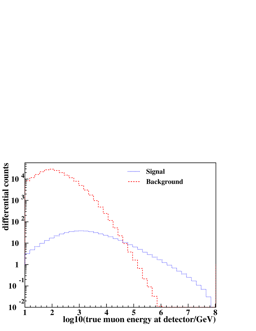
Figure 2: Differential energy distribution of true muon energies in a neutrino detector for the atmospheric neutrino flux and an $E^{-2}$ diffuse neutrino flux, of level $E^{2}\Phi_{90}=3\times 10^{-8}\;\mathrm{GeV}\;\mathrm{cm}^{-2}\;\mathrm{s}^{-1}\;\mathrm{sr}^{-1}$, corresponding to the Waxman-Bahcall upper bound calculation.

Figure 3 shows the integrated event rates above each muon energy. For each value of the expected atmospheric neutrino background, we can calculate the average upper limit that would be obtained by the experimental ensemble with no true signal, and this curve is added to the plot as a solid line.

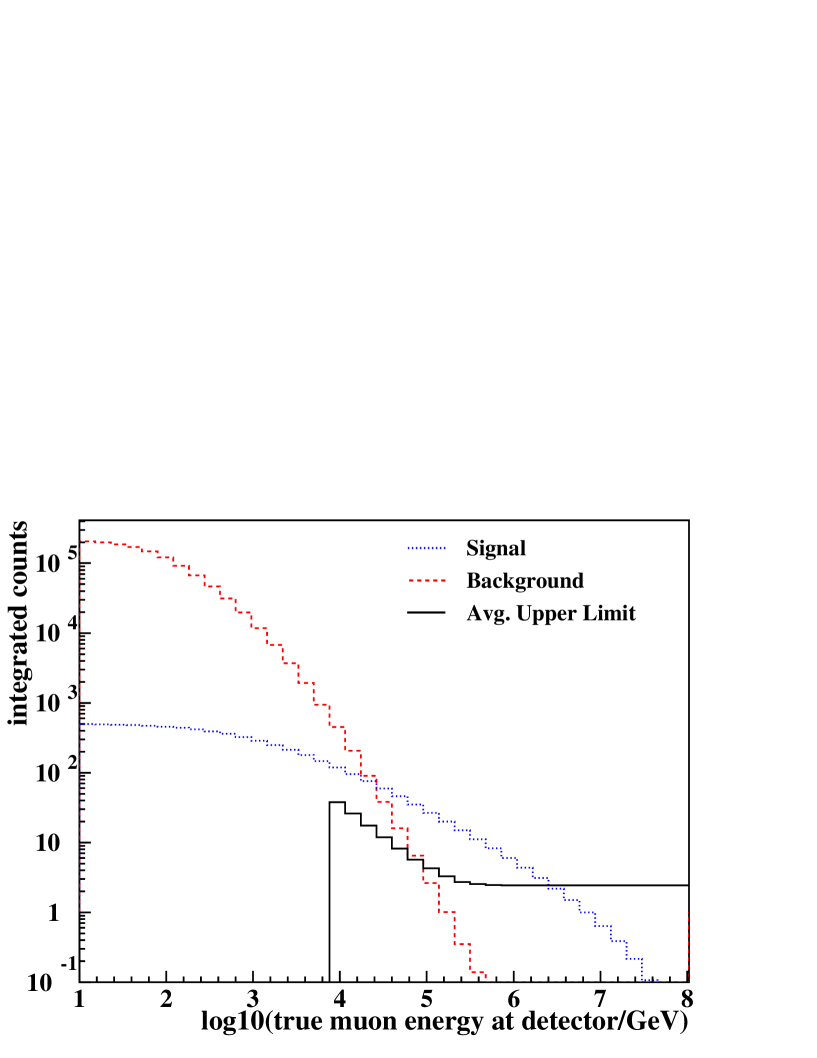
Figure 3: Integrated energy distribution of true muon energies for the fluxes shown in figure 2. The average upper limit that would be obtained by an ensemble of experiments with no true signal and only the expected atmospheric neutrino background is shown by the solid line. If the background exceeds 700, we do not calculate an average upper limit, thus the cut off in the curve at $\log_{10}(E_{\mu})=3.87$.

As the background decreases the average upper limit reduces toward 2.44, the value of $\mu_{90}(n_{\mathit{obs}},n_{b})$ for $n_{b}=0$ and $n_{\mathit{obs}}=0$. Clearly, if $n_{b}=0$, the only non-zero term in the sum in equation 4 is $\mu_{90}(0,0)=2.44$ which occurs with probability one (if the background is zero, then the only possible observation in the absence of signal is $n_{\mathit{obs}}=0$). The best cut corresponds to the muon energy above which the ratio of the average upper limit to the expected diffuse signal is minimised. This is shown in figure 4. The best cut lies close to a muon energy of $10^{5}$ GeV, where 2.64 background and 26.69 signal events remain. The average upper limit for this expected background is 4.26, leading to a model rejection factor for the assumed flux strength of $4.26/26.69=0.16$, and thus a limit on such an $E^{-2}$ flux of

$$E^{2}\Phi_{90}<4.8\times 10^{-9}\;\mathrm{GeV}\;\mathrm{cm}^{-2}\;\mathrm{s}^{-1}\;\mathrm{sr}^{-1}$$ (8)

This level of sensitivity is nearly an order of magnitude below that of the Waxman-Bahcall bound.

Note that this procedure is independent of the assumed signal strength, depending only the shape of the signal spectrum.

Figure 4: Model rejection factor, $\bar{\mu}/n_{s}$, for a diffuse flux search in a kilometre effective area neutrino telescope, as a function of the muon energy cut. The best average limit on the source flux occurs where the MRF is minimised, here at a muon energy just below $10^{5}$ GeV.

This limit is an ideal one where we have assumed we can measure the muon energy exactly. A realistic detector will have a finite energy resolution, and we incorporate this by assuming a gaussian resolution in the logarithm of the true muon energy. Table 1 shows a summary of the model rejection potential optimisations for measurements of the true muon energy, for several assumed detector muon energy resolutions, and for measurements of the true neutrino energy, which would indicate the best possible limit that the detector could achieve. Also, we show what constraints would be placed on other models of neutrino production, using as examples the calculation of Stecker, Done, Salamon and Sommers [23] (SDSS), and one of the diffuse bounds of Mannheim, Protheroe and Rachen [22] (MPR). A logarithmic muon energy resolution of 30% produces an expected limit below the Waxman-Bahcall upper bound, and is sufficient to place strong constraints on both the SDSS and MPR models.

The effects of increasing the detector exposure time are shown in table 2, where three years of livetime exposure is assumed. In each case the optimisation moves toward higher energy cut values, and the improvement in the expected limits goes approximately as the square root of the exposure time. The detector performance for three years exposure is also summarised in figure 5.

Table 1: Model rejection potential results for various astrophysical neutrino spectra, for one year live time in a kilometre scale neutrino detector. The Waxman-Bahcall flux limits are in units $\mathrm{GeV}\;\mathrm{cm}^{-2}\;\mathrm{s}^{-1}\;\mathrm{sr}^{-1}$.

	cut		above cut
Flux	var.($\log$ err.)	$\log_{10}E$	$n_{s}$	$n_{b}$	$\bar{\mu}(n_{b})$	Flux limit ($=\Phi\times\frac{\bar{\mu}}{n_{s}}$)
	$E_{\nu}(0\%)$	5.68	51.12	1.25	3.45	$2.03\;.\;10^{-9}$
	$E_{\mu}(0\%)$	4.96	26.69	2.64	4.26	$4.79\;.\;10^{-9}$
WBUB	$E_{\mu}(10\%)$	5.32	18.77	4.12	4.87	$7.79\;.\;10^{-9}$
	$E_{\mu}(20\%)$	5.68	18.47	22.19	9.37	$1.52\;.\;10^{-8}$
	$E_{\mu}(30\%)$	6.40	14.09	32.15	10.98	$2.35\;.\;10^{-8}$
	$E_{\nu}(0\%)$	5.86	281.40	0.47	2.83	$\Phi_{\mathrm{MPR}}\times 1.01\;.\;10^{-2}$
	$E_{\mu}(0\%)$	5.14	127.58	1.01	3.29	$\Phi_{\mathrm{MPR}}\times 2.58\;.\;10^{-2}$
MPR	$E_{\mu}(10\%)$	5.50	90.10	1.99	3.94	$\Phi_{\mathrm{MPR}}\times 4.37\;.\;10^{-2}$
	$E_{\mu}(20\%)$	6.22	54.55	4.51	5.01	$\Phi_{\mathrm{MPR}}\times 9.18\;.\;10^{-2}$
	$E_{\mu}(30\%)$	6.94	40.53	9.09	6.51	$\Phi_{\mathrm{MPR}}\times 0.161$
	$E_{\nu}(0\%)$	5.68	3347.49	1.25	3.45	$\Phi_{\mathrm{SDSS}}\times 1.03\;.\;10^{-3}$
	$E_{\mu}(0\%)$	5.14	1222.01	1.01	3.29	$\Phi_{\mathrm{SDSS}}\times 2.69\;.\;10^{-3}$
SDSS	$E_{\mu}(10\%)$	5.32	1039.62	4.12	4.87	$\Phi_{\mathrm{SDSS}}\times 4.69\;.\;10^{-3}$
	$E_{\mu}(20\%)$	6.04	606.97	7.40	6.01	$\Phi_{\mathrm{SDSS}}\times 9.91\;.\;10^{-3}$
	$E_{\mu}(30\%)$	6.76	452.29	14.07	7.77	$\Phi_{\mathrm{SDSS}}\times 1.72\;.\;10^{-2}$

Table 2: Model rejection potential results for various astrophysical neutrino spectra, for three years live time in a kilometre scale neutrino detector. The Waxman-Bahcall flux limits are in units $\mathrm{GeV}\;\mathrm{cm}^{-2}\;\mathrm{s}^{-1}\;\mathrm{sr}^{-1}$.

	cut		above cut
Flux	var.($\log$ err.)	$\log_{10}E$	$n_{s}$	$n_{b}$	$\bar{\mu}(n_{b})$	Flux limit ($=\Phi\times\frac{\bar{\mu}}{n_{s}}$)
	$E_{\nu}$ (0%)	5.86	118.56	1.40	3.55	$8.99\;.\;10^{-10}$
	$E_{\mu}(0\%)$	5.14	60.21	3.04	4.43	$2.21\;.\;10^{-9}$
WBUB	$E_{\mu}(10\%)$	5.50	43.12	6.01	5.53	$3.85\;.\;10^{-9}$
	$E_{\mu}(20\%)$	6.04	35.48	22.06	9.34	$7.90\;.\;10^{-9}$
	$E_{\mu}(30\%)$	6.58	34.73	62.20	14.82	$1.28\;.\;10^{-8}$
	$E_{\nu}(0\%)$	6.04	690.04	0.52	2.88	$\Phi_{\mathrm{MPR}}\times 4.17\;.\;10^{-3}$
	$E_{\mu}(0\%)$	5.32	311.16	1.06	3.32	$\Phi_{\mathrm{MPR}}\times 1.07\;.\;10^{-2}$
MPR	$E_{\mu}(10\%)$	5.68	219.77	2.84	4.35	$\Phi_{\mathrm{MPR}}\times 1.98\;.\;10^{-2}$
	$E_{\mu}(20\%)$	6.58	112.87	4.33	4.94	$\Phi_{\mathrm{MPR}}\times 4.38\;.\;10^{-2}$
	$E_{\mu}(30\%)$	7.12	103.89	18.42	8.65	$\Phi_{\mathrm{MPR}}\times 8.32\;.\;10^{-2}$
	$E_{\nu}(0\%)$	5.86	8076.81	1.40	3.55	$\Phi_{\mathrm{SDSS}}\times 4.40\;.\;10^{-4}$
	$E_{\mu}(0\%)$	5.32	2841.39	1.06	3.32	$\Phi_{\mathrm{SDSS}}\times 1.17\;.\;10^{-3}$
SDSS	$E_{\mu}(10\%)$	5.50	2481.94	5.96	5.52	$\Phi_{\mathrm{SDSS}}\times 2.22\;.\;10^{-3}$
	$E_{\mu}(20\%)$	6.40	1217.47	7.67	6.09	$\Phi_{\mathrm{SDSS}}\times 5.00\;.\;10^{-3}$
	$E_{\mu}(30\%)$	7.12	967.18	17.89	8.54	$\Phi_{\mathrm{SDSS}}\times 8.83\;.\;10^{-3}$

Figure 5: Summary of the limit setting potential of a kilometre-scale neutrino detector after three years of operation. For each of the diffuse flux models under consideration, the highest curves show the predicted neutrino flux. The shaded bands correspond to the expected range of the limit for different assumptions of the muon energy resolution of the detector, the upper edge of the band corresponding to 30% logarithmic muon energy resolution, and the lower edge, perfect muon energy resolution. The lowest curves for each flux show the expected limits if the neutrino energy could be measured directly. The atmospheric neutrino background is also shown as a band representing the flux variation from horizontal (top of band) to vertical (bottom of band) arrival directions.

4.2 Model rejection potential optimisation for point source searches

In the search for a point source, we can reduce the background to the search by cutting on both the energy of the events, and also on the angular acceptance window about the known direction of the source. We apply the model rejection potential procedure in two dimensions, producing a two dimensional surface of model rejection factor, $\bar{\mu}/s$, in the energy and angular acceptance ($\Delta\Psi$ degrees about the known direction) cut variables. As a single illustration of this technique, a contour plot representation of this surface for the case of an $E^{-2}$ point source, assuming an angular resolution with Gaussian $\sigma=3.0^{\circ}$, and an exact measure of the muon energy in the detector, is shown in figure 6. The best constraint on the $E^{-2}$ point source (shown as a cross) is found by accepting events with $\Delta\Psi<3.8^{\circ}$ and $\log 10(E_{\mu}/\mathrm{GeV})>4.5$. The remaining background of 1.4 events leads to an average event upper limit of 3.56 and an optimised flux limit of

$$E^{2}\Phi_{90}<9.4\times 10^{-10}\;\mathrm{GeV}\;\mathrm{cm}^{-2}\;\mathrm{s}^{-1}\;$$ (9)

The change in model rejection factor moving between adjacent contours corresponds to a change in the average flux upper limit in linear steps of $10^{-10}\;\mathrm{GeV}\;\mathrm{cm}^{-2}\;\mathrm{s}^{-1}\;$. Thus the minimum lies in a fairly broad range in the two dimensional cut parameter space.

If we assume a 30% logarithmic muon energy resolution, the optimal cuts change to $\Delta\Psi<2.5^{\circ}$ and $\log 10(E_{\mu}/\mathrm{GeV})>3.25$, and the limit is only a factor of 2.5 weaker than for the true energy measurement case. Contrast this to the diffuse $E^{-2}$ limit case, where the 30% energy resolution produced a limit a factor of 4.9 weaker, due to sole reliance of energy as the cut. In the point source case, much of the background rejection comes from the angular acceptance cut, and the energy measurement error has less effect.

Figure 6: Surface of model rejection factor, $\bar{\mu}/n_{s}$, for a point source search in a kilometre effective area neutrino telescope, where the angular acceptance about the assumed source direction, and the true detector muon energy are used as cut parameters. Adjacent contours correspond to a change in the flux upper limit of $10^{-10}$, with the minimum value of $9.4\times 10^{-10}\;\mathrm{GeV}\;\mathrm{cm}^{-2}\;\mathrm{s}^{-1}\;$ indicated by the cross.

4.3 Model rejection potential optimisation for gamma-ray burst searches

The mechanisms that power gamma-ray bursts are still not determined. If hadronic acceleration mechanisms are producing gamma-rays via proton interactions and subsequent neutral pion decay, then there should also be fluxes of high energy neutrinos. Large neutrino detectors will look for these neutrinos in coincidence with the satellite observations of the gamma-rays. Waxman and Bahcall [21] compute the expected neutrino flux by assuming that the gamma-ray bursts are also the source of the observed cosmic rays.

Just as in the point source search we optimise both the angular acceptance about the known source direction and the true muon energy. The additional cut on a time window about the known GRB time greatly reduces the background to the search. We assume that we will test a model in which the neutrinos are produced within 10 seconds of the burst time. The accumulated number of coincident bursts is used as a measure of the detector exposure [29].

The model rejection factor surface after 500 satellite-coincident bursts are seen in the detector’s field of view is shown in figure 7. The application of a 10 second time window cut about each of the known burst times reduces the total background to essentially zero and thus only loose cuts are needed – an angular acceptance cut of $\Delta\Psi<7.0^{\circ}$ and an energy cut of $\log 10(E_{\mu}/\mathrm{GeV})>1.18$, both of which are much weaker than for the point source optimisation of section 4.2, are found to be optimal. Using these cuts, the remaining atmospheric background (0.17 events) and average upper limit (2.58) lead to an optimal upper limit corresponding to a flux of 0.18 times that of the Waxman-Bahcall prediction. Again, the minimum lies in a broad region – the change in model rejection factor between adjacent contours being $6.7\times 10^{-3}$. Since the background is so close to zero, the limit will tend to scale linearly with an increase in the number of observed bursts.

Incorporating a realistic 30% logarithmic muon energy resolution leads to a model rejection factor of 0.3, again only a factor of 1.7 worse than the ideal muon energy measurement case. The cuts stay close to those of the ideal case, with $\Delta\Psi$ of $7.5^{\circ}$, and the energy cut loosened to accept all simulated events ($\log 10(E_{\mu}/\mathrm{GeV})>1.0$) leading to an expected background of 0.12 and average event upper limit of 2.54. Due to the addition of the time cut, the energy measurement error has even less weakening effect on the optimal limit than in the point source case.

Figure 7: Surface of model rejection factor, $\bar{\mu}/n_{s}$, for a Waxman-Bahcall model gamma-ray burst source search in a kilometre effective area neutrino telescope, where, in addition to angle and energy cuts, a time window cut of 10 seconds about each of the assumed 500 known GRB emission times is applied. The point of the minimum model rejection factor of 0.18 is indicated by the cross.

5 Conclusions

In this paper we have described a method of choosing experimental cuts in order to maximise the chance of placing the strongest possible constraint on an expected signal model. Choosing the experimental cuts to optimise the model rejection factor (ratio of expected average upper limit to expected signal) is shown to yield the best average constraint on the signal model. We have demonstrated this method by determining the sensitivity of kilometre-scale neutrino detectors to diffuse and point sources of astrophysical neutrinos, and find that such detectors will strongly constrain present models. We suggest that the optimised average flux upper limits described here be used as a standard method of comparing the capabilities of different neutrino detectors.

References

- [1] G.C. Hill, Talk given at Brussels AMANDA collaboration meeting, May 2000
- [2] G.C. Hill and K. Rawlins, Presentation at NSF Hartill Icecube Review, June 2000
- [3] J. Neyman, Phil. Trans. Royal Soc. London, Series A, 236 333-80 (1937).
- [4] G.J. Feldman and R.D. Cousins, Phys. Rev. D57 3873 (1998)
- [5] R.D. Cousins, Am. J. Phys. 63 (5) 398 (1994)
- [6] For recent updates on large neutrino detectors, see the Proceedings of the 27th International Cosmic Ray Conference, Hamburg, (2001)
- [7] W. Rhode et al., Astropart. Phys., 4, 217, 1996.
- [8] E. Zas, F. Halzen and R.A. Vázquez Astropart. Phys. 1 (1993) 297
- [9] T.K. Gaisser, F.Halzen, and T.Stanev. Phys. Rep. 258 (1995) 173
- [10] G.M. Frichter, D.W. McKay, and J.P. Ralston. Phys. Rev. Lett. 74 (1995) 1508
- [11] G.M. Frichter, D.W. McKay, and J.P. Ralston. Phys. Rev. D 53 (1996) 1684
- [12] R. Gandhi et al., Astropart. Phys. 5 (1996) 81-110
- [13] G.C. Hill, PhD thesis, University of Adelaide (1996)
- [14] G.C. Hill, Astropart. Phys. 6 (1997) 215
- [15] R. Gandhi et al., Phys.Rev D 58 (1998) 093009
- [16] I.F.M. Albuquerque, J. Lamoureux and G.F. Smoot, Ap. J.S. in press (hep-ph 0109177) (2001)
- [17] A.D. Martin, W.J. Stirling, and R.G. Roberts, Phys. Lett. B 354 (1995) 155
- [18] P. Lipari and T. Stanev, Phys. Rev. D 44 (1991) 3543
- [19] A.M. Dziewonski and D.L. Anderson, Phys. Earth Planet. Inter. 25 (1981) 297
- [20] Icecube collaboration, in preparation (2002)
- [21] E. Waxman and J. Bahcall, Phys. Rev. D 59 (1999) 023002
- [22] K. Mannheim, R.J. Protheroe and J.P. Rachen, Phys. Rev. D 63 (2001) 023003
- [23] F.W. Stecker, C. Done, M.H. Salamon, and P. Sommers, Phys. Rev. Lett. 66 (1991) 2697, Errata Phys. Rev. Lett. 69 (1992) 2738
- [24] P. Lipari, Astropart. Phys. 1 (1993) 195
- [25] C.G.S. Costa, Astropart. Phys. 16 (2001) 193
- [26] T.K. Gaisser and M. Honda, to appear in Ann. Rev. of Nuclear and Particle Science 52 (2002) (hep-ph 0203272)
- [27] R.D. Cousins and V.L. Highland, Nucl. Inst. Meths. A320 (1992) 331
- [28] J. Conrad et al., submitted to Phys. Rev. D (2002) hep-ex 0202013
- [29] T.R. DeYoung and A. Karle, private communication (2001)