Toward An Empirical Theory of Pulsar Emission VIII: Subbeam Circulation and the Polarization-Modal Structure of Conal Beams

Abstract

The average polarization properties of conal single and double profiles directly reflect the polarization-modal structure of the emission beams which produce them. Conal component pairs exhibit large fractional linear polarization on their inside edges and virtually complete depolarization on their outside edges; whereas profiles resulting from sightline encounters with the outer conal edge are usually very depolarized. The polarization-modal character of subbeam circulation produces conditions whereby both angular and temporal averaging contribute to this polarization and depolarization.

These circumstances combine to require that the circulating subbeam systems which produce conal beams entail paired PPM and SPM emission elements which are offset from each other in both magnetic azimuth and magnetic colatitude. Or, as rotating subbeam systems produce (on average) conal beams, one modal subcone has a little larger (or smaller) radius than the other. However, these PPM and SPM “beamlets” cannot be in azimuthal phase, because both alternately dominate the emission on the extreme outer edge of the conal beam. While this configuration can be deduced from the observations, simulation of this rotating, modal subbeam system reiterates these these conclusions. These circumstances are also probably responsible, along with the usual wavelength dependence of emission height, for the observed spectral decline in aggregate polarization.

A clear delineation of the modal polarization topology of the conal beam promises to address fundamental questions about the nature and origin of this modal emission—and the modal parity at the outer beam edges is a fact of considerable significance. The different angular dependences of the modal “beamlets” suggests that the polarization modes are generated via propagation effects. This argument may prove much stronger if the modal emission is fundamentally only partially polarized. Several theories now promise quantitative comparison with the observations.

The Outer-Edge Depolarization Phenomenon

A humble fact about pulsar radio emission, which to our knowledge has attracted virtually no notice or comment, is the following: The extreme outer edges of virtually all conal component pairs are prominently, and apparently accurately, depolarized. Considerable comment has been made regarding the obverse of this circumstance—that is, to the effect that the highest levels of fractional linear polarization are usually found on the inner edges of conal components, indeed where it is sometimes nearly complete (Manchester 1971; Morris et al 1981).

Of course, longitudes corresponding to the outer edges of such conal component pairs are also just where intervals of secondary polarization-mode dominance are seen in individual pulses, as we know from those well known stars whose profiles indicate a fairly central sightline traverse through the conal beam: B0329+54 exhibits zones of outer edge depolarization over a wide frequency range (Gould & Lyne 1998; hereafter GL98; Suleymanova & Pugachev 1998, 2002) accompanied by prominent outer edge “90^∘ flips” in the position angle (PA). Earlier average studies (Manchester 1971; Morris et al 1981; Bartel et al 1982) together with the more recent single-pulse analyses of Gil & Lyne (1995), von Hoensbroech & Xilouris et al (1997), and Mitra (1999) provide an unusually comprehensive picture of this pulsar’s outer edge depolarization. The phenomenon persists to the highest frequencies, as can clearly be seen in the 10.55-GHz profile of von Hoensbroech & Xilouris above.

Figure 1: Log-linear plots of the polarized intensity profiles of pulsar B1133+16, showing the full extent of the edge depolarization—430 MHz (upper) and 1414 MHz (lower). The total intensity, Stokes parameter $I$, is given by the solid curve, the linear polarization $L$ by the dashed curve, and $-V$ by the dotted one (only rh circular is observed in this pulsar). The three respective curves were smoothed over five samples, normalized to the maximum in $I$, and the statistical bias in $L$ was removed. The 430-MHz and 21-cm sequences had lengths of 956 and 2180 pulses, respectively.

Other obvious exemplars are pulsars B0525+21 and 1133+16, which clearly exhibit the outer edge depolarization phenomenon over the entire range of frequencies that they can be observed [see the above papers as well as Blaskiewicz et al (1991), von Hoensbroech (1999), and Weisberg et al (1999)]. For 0525+21, which has a more central sightline traverse (see Table 1), individual-pulse polarization displays show that the weaker secondary polarization mode dominates the primary one (hereafter SPM and PPM, respectively) only on the extreme outer edges of its profiles; whereas for 1133+16, which has a more oblique sightline traverse, SPM dominated samples can be seen over a larger longitude range.

Reference to the now extensive body of published average polarimetry provides several hundred examples of pulsars whose conal component pairs have prominently depolarized outer edges. The effect is so widespread, indeed, that it is difficult to identify completely convincing examples to the contrary. The stars comprising four of the five main profile classes (e.g., see Paper VI) of conal single (S_d), double (D), triple (T), and five-component (M) virtually all exhibit the phenomenon as do the few stars in the more restricted cT and cQ classes. It is worth noting that good examples of outer edge depolarization are found among stars with both inner and outer conal configurations; all three of the stars with inner cones discussed in the foregoing Paper VII [Mitra & Rankin (2002)] show the effect, though interestingly, in each case it is more prominent on the trailing than on the leading edge. The best examples of stars with little or no edge depolarization all either have (or probably have, given that some are yet not well observed) core single S_t or inner-cone triple T configurations; some are B0355+54, 0450+55, 0540+23, 0559–05, 0626+24, 0740–28, 0833–45, 0906–49 (main pulse), 1055–52, 1322+83, and 1737–30, and note that, overall, these stars have much shorter periods than is typical for the normal pulsar population.

We then summarize the overall characteristics of the edge-depolarization phenomenon:

1. The average linear polarization $L$ (=$\sqrt{Q^{2}+U^{2}}$) falls off much faster than the total power $I$ on the edges of the profile and decreases asymptotically to near zero.

2. This phenomenon usually occurs over a very broad band—essentially the entire range of the observations—and therefore, the edge depolarization appears to be nearly independent of frequency.

3. This profile-edge depolarization is modal in origin, meaning that it largely occurs through the incoherent addition of PPM and SPM power both within samples and from pulse to pulse.

4. The edge depolarization affects conal component pairs, and therefore must be regarded as a roughly symmetrical, structural feature of conal emission beams.

5. Then, in terms of such beams:

   • the outer edge depolarization requires that the modal power be about equal at large angles to the magnetic axis, and

   • the proximity of the depolarized outer edges of conal component pairs to their more highly polarized inner edges requires that the weaker mode peak at slightly larger angles to the magnetic axis than the stronger one.

In the remainder of this paper we will explore the causes and consequences of these circumstances, drawing extensively on the earlier articles of this series, Papers I–VII (see References). We will show that these structural characteristics of conal emission beams—and therefore well resolved conal component pairs—are almost certainly the result of subbeam circulation as in pulsar B0943+10 (see Deshpande & Rankin 2001). This circulation, in sweeping a series of polarized subbeams around the magnetic axis and past our sightline, is responsible for the outer-edge depolarization and (sometimes periodic) modal fluctuations in pulsars where the sightline traverse cuts the emission beam centrally (e.g., 0525+21); it is also largely responsible for the very different polarization effects observed in pulsars where the sightline traverse is oblique (i.e., B0809+74). Of course, only subbeams with particular angular polarization patterns can produce the particular sorts of depolarized profile forms that are observed, and in the remainder of this paper we endeavor to understand what general features are required of them. In the following sections, we first briefly describe our observations and then consider the contrasting characteristics of stars, first with well separated conal component pairs, and then with conal single S_d profiles. The penultimate section gives the results of modelling the polarized emission beam, and we conclude with a summary of our results and a discussion of their implications.

Observations

Table 1: Pulsar Parameters.

Pulsar	$P$	$\beta/\rho$	$f$	Source	Date	BW
(B–)	(s)		(MHz)			(MHz)
0301+19	1.388	0.45	430	AO	1974Jan5	10/32
0329+54	0.715	0.31	840	WSRT	2002Jan10	80/512
0525+21	3.745	0.19	430	AO	1974Apr4	10/32
1133+16	1.188	0.78	430	AO	1992Oct19	10/32
			1414	AO	1992Oct15	20/32
1237+25	1.382	$\sim$0	430	AO	1974Jan6	10/32
2020+28	0.343	0.49	430	AO	1992Oct16	10/32
0809+74	1.292	$0.93$	328	WSRT	2000Nov26	10/64
0820+02	0.865	$0.98$	430	AO	1992Oct19	10/32
0943+10	1.098	-1.01	430	AO	1992Oct19	10/32
1923+04	1.074	$0.97$	430	AO	1991Jan6	10/32
2016+28	0.558	$0.96$	430	AO	1992Oct15	10/32
2303+30	1.576	$0.99$	430	AO	1992Oct15	10/32

The source and character of our observations are summarized in Table 1. The Arecibo Observatory (AO) recordings were made under two polarimetry programs, the first in the early 1970s and the second in 1992, and both are described in Rankin & Rathnasree (1997). The 328- and 840-MHz sequences were made using the Westerbork Synthesis Radio Telescope (WSRT) with its pulsar machine PuMa, and these are described in Ramachandran et al (2002).

The Depolarization Pattern of Conal Component Pairs

Figure 2: Three-way, mode-segregated average profiles for pulsars with prominent conal component pairs, B0301+19, 0329+54, 0525+21, 1133+16, 1237+25, and 2020+28. The heavier solid and dashed curves give the total power (Stokes $I$) and total linear $L$; whereas, the lighter dashed, dotted and solid curves give the PPM, SPM and UP power, computed according to the algorithm in Deshpande & Rankin’s (2001) Appendix (see text).

Figure 3: Three-way, mode-segregated average profiles for six conal single S_d pulsars, B0809+74, 0820+02, 0943+10, 1923+04, 2016+28, and 2303+30 as in Fig. 2.

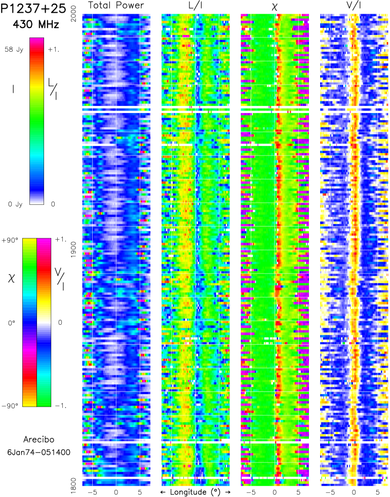
Figure 4: Color polarization display of a 200-pulse portion of the 430-MHz observation in Figs. 2 and 5. The first column gives the total intensity (Stokes $I$), with the vertical axis representing the pulse number and the horizontal axis pulse longitude, colour-coded according to the left-hand scale of the top bar to the left of the displays. The second and third columns give the corresponding fractional linear polarization ($L/I$) and its angle ($\chi={1\over 2}\tan^{-1}{U/Q}$), according to the top-right and bottom-left scales. The last column gives the fractional circular polarization ($V/I$), according to the bottom-right scale. Plotted values have met a threshold corresponding to 2 standard deviations of the off-pulse noise level. Note the 2.63 c/$P_{1}$ modulation associated with the outer conal component pair—and that this modulation has a strikingly modal character as can be seen particularly clearly in the orthogonal chartreuse and magenta PAs.

Let us now look in more detail at the manner in which the outer edges of conal component pairs are depolarized. Turning first to pulsar 1133+16, Figure 1 shows the relative behaviors of the logarithms of Stokes parameters $I$, $L$, and $-V$ as a function of longitude for a 430-MHz sequence (top) and a 21-cm sequence (bottom). Here we can follow the behavior of the fractional polarization far out into the “wings” of the star’s profile. We see not only that the depolarization persists to very low intensity levels, but also that its linear and circular polarization generally decrease with or faster than the total power down to the point where the noise fluctuations begin to dominate at 2–4$\times$10^-4 (note that only the absolute value of the noisy quantities can be plotted).

Probably, this behavior is typical of many pulsars, but only for a few, such as 1133+16, can polarized profiles with such a large dynamic range be computed. Even for 1133+16 it would be interesting to compute a more sensitive such display. These observations from Arecibo were only some 40 minutes long, so with care it should be possible to reduce the relative noise level much further. If, then, it is generally true that the outer edges of conal profiles—and thus the outer edges of conal beams—are accurately depolarized on average, it provides a strong constraint on the angular beaming characteristics of the modal emission.

We can look at this outer-edge depolarization in more detail by conducting an appropriate mode-segregation analysis on selected sequences. Two such algorithms were described in Deshpande & Rankin’s (2001) Appendix, and we use here the three-way mode segregation method, because it provides the greatest flexibility. It produces two fully polarized PPM and SPM pulse sequences and a fully depolarized UP sequence, while making no restrictive assumptions about the origin of the depolarization. Briefly, the $I$ and $L$ of each sample are compared with a noise threshold, and its respective $L$ and $I$–$L$ portions accumulated in three partial sequences depending on whether the sample is PPM dominated, SPM dominated (relative to a model PA traverse which defines the former), or essentially unpolarized (UP).

The results of these analyses for pulsars with prominent conal component pairs are given in Figure 2, where the heavier curves give the usual total-power ($I$) and total linear ($L$) profiles, while the lighter curves show the PPM (dashed curve), SPM (dotted curve) and UP (solid curve) profiles. A similar (but more primitive) analysis for B1737+13 (Rankin et al 1986) can also be compared, as can the excellent modal polarization studies of B2020+28 and 0525+21 by McKinnon & Stinebring (1998, and 2000, respectively; hereafter MS98 and MS00). The sources of the various sequences are given in Table 1, where we also tabulate $\beta/\rho$. For the stars considered in this section, $|\beta|/\rho<0.8$, a sightline geometry which produces well resolved conal component pairs. Note, by contrast, that the conal single S_d pulsars considered in the next section all have $|\beta|/\rho>0.9$.

For most of the stars (all but B2020+28), we see a fairly consistent picture. The weaker mode only rarely has sufficient intensity to dominate a sample, so the aggregate SPM power is typically only some 10% that of the PPM—and almost all of this SPM power is found on the “wings” of the profiles. Often, the SPM power peaks slightly further out than the PPM and exhibits a narrower angular width. Note, further, that the UP distribution behaves very similarly to both the PPM and SPM curves, so we may view some portion of the UP power as the accumulation of samples which were depolarized by equal contributions of PPM and SPM power—and indeed, the UP curves always asymptotically approach the overall $I$ curves at very low power levels. This behavior could also be demonstrated by applying the two-way modal “repolarization” technique in Deshpande & Rankin, which proceeds under the assumption that the depolarized samples contain equal PPM and SPM levels of power.

Though pulsar 2020+28’s modal behavior appears more complex (e.g., Cordes et al 1978; MS98), we see many of the same features—for instance, that the UP power approaches the total power on the extreme edges of profile. Indeed, MS98’s analysis based on “superposed modes” suggests similar conclusions. The well measured profile demonstrates that its “two” components each have a good deal of structure—seen as “breaks” in the total-power curves—but the PPM, SPM and UP curves demonstrate, in addition, that much of the complexity is modal in origin. The complex modal behavior of this pulsar deserves much fuller study, and a well measured polarimetric pulse sequence in the 100–200-MHz range would add much to our knowledge.

Overall, we see that the conal component pairs depicted in Figure 2 all have moderate to high levels of fractional linear polarization—that is, typically some 50%—though most have narrow, interior regions of longitude where the linear polarization is higher. We shall see that this stands in sharp contrast to the S_d pulsars considered in the following section. Our point is that when $|\beta|/\rho$ is relatively small—producing well resolved conal component pairs—the mode mixing depolarizes the outer edges, but not the profile interior. This then reflects properties—both dynamic in terms of modulation phenomena and polarizational—of the conal emission beam, and we must reflect on just how this is possible.

The Depolarization Patterns of Conal Single Stars

We have just considered a group of stars in which our sightline makes a fairly central traverse through their emission cone(s), and we now turn to members of the conal single S_d group, all of which are configured by a tangential traverse along the average emission cone. Here we have the opportunity both to explore the conal depolarization phenomena in a very different geometrical context and then to investigate how the modulation and depolarization phenomena are connected. Figure 3 gives mode-segregated polarization plots (similar to those in Fig. 2) for six S_d stars. Here, it is important to keep in mind that each of these pulsars has prominent “drifting” subpulses, so that the profiles give only a static average of the subpulse polarization. The displays of Fig. 3 show that the UP (perhaps, mode-mixed) power is typically 50% of the total, so that the overall modal contributions are comparable and the aggregate linear polarization is often small. While all of the total-power profiles are roughly unimodal (only B0820+02 is really symmetrical), the modal profiles are more complex; the two peak at different longitudes in B0809+74; the SPM has a double form in B2016+28; and we have already noted the peculiar “triple” form of the aggregate linear in pulsar 0820+02.

As a class, the S_d stars exhibit conspicuously depolarized profiles at metre wavelengths. Indeed, this has been one of the great obstacles to understanding their characteristics, because, for many (i.e., 0809+74), the modal complexity and low fractional linear polarization make it difficult to accurately determine even such a simple parameter as the PA sweep rate (e.g., Ramachandran et al 2002). Paradoxically, some also have nearly complete linear polarization at certain longitudes and frequencies (i.e., as does 0809+74’s leading edge at higher frequencies) suggesting that mode-mixing is not always operative.

The S_d pulsars are also the profile class most closely associated with the problematic phenomenon of “absorption”. It was in 0809+74 that the effect was first identified (Bartel et al 1981; Bartel 1981)—that is, evidence that parts of the profiles were “missing”—and strong evidence to this effect through subbeam-mapping methods have also been adduced for 0943+10 (Deshpande & Rankin 2001). Surely one could imagine from 0943+10’s asymmetric profile that a part of its trailing-edge emission is “absorbed”, though 0809+74’s more symmetric leading edge at meter wavelengths gives little clue that emission appears to be missing here as well. In short, the circumstances defining the profile edges appear to be more complicated for conal single stars than for the other species, and their modal polarization characteristics are an aspect of this complexity.

What is the Relative Polarization-Modal Phase in Conal Component Pairs?

We have learned in the foregoing two sections that well resolved conal component pairs are most depolarized on their extreme outer edges, while the polarized modal emission in conal single stars accrues to the depolarization essentially over the entire width of the profile. These circumstances begin to illuminate the polarization configuration of the subbeams; and, indeed, we saw in Deshpande & Rankin (2001; fig. 19) that for 0943+10 the discernible SPM emission was found in between the 20 PPM subbeams. We have found a similar configuration for pulsar 0809+74, where the PPM and SPM power centers are displaced from each other systematically in both magnetic azimuth and colatitude by perhaps 20% of the subbeam spacing (Rankin et al 2002).

A related question which has had no investigation at all is the following: what is the modulation phase relationship between the PPM and SPM power on the outside edges of pulsars with conal component pairs? Such a question is not trivial to answer because only a few of such stars have modal modulation which is strongly periodic (while virtually all of the S_d stars, for instance, in Fig. 2 exhibit a good deal of regularity). Two pulsars which do have periodic modulation features are B1237+25 and 2020+28.

Figure 5: Modulation amplitude and phase of the three-way segregated PPM (top) and SPM (bottom) power in pulsar B1237+25 at 2.63 c/$P_{1}$. Note that 40–60% of the fluctuation power under the outer cone is modulated at this frequency and that the modal sequences have roughly opposite phases. The relationship at other longitudes is difficult to interpret, because the mode segregation is less definitive and the fluctuating power small or negligible. The sequence here is a superset of that in Fig. 2.

Figure 4 exhibits the character of this subpulse modulation in pulsar B1237+25. This sequence was chosen for its brightness and relative freedom from nulls, and in consequence its outer components show a particularly sharp feature at 2.63 c/$P_{1}$. This modulation can be seen very clearly in the first column which gives the total power $I$. The modal character of the modulation, however, is most obvious in the third column depicting the PA, where the alternating magneta and chartreuse colors represent orthogonal PAs. Further effects of this modal modulation can be seen in the varying levels of associated depolarization (second column) and the correlated variations of circular polarization (forth column). Note that virtually all of these modal modulation effects are confined to the outermost pair of conal components, usually referred to as components I and V.

Figure 5 provides a more quantitative analysis of this modal modulation under B1237+25’s outer conal component pair. The top display gives the PPM profile after a three-way segregation of the modal power along with a curve showing the fraction of this power which is modulated at the feature frequency of 2.63 c/$P_{1}$; whereas the lower panel gives the phase of this modulation. As noted above, we chose a part of the pulse sequence with few nulls, which also had a particularly “pure” modulation feature. Clearly, the phase is only reliable under the outside conal component pair, where the modulation represents a large fraction of the total modal power. The lower display gives similar information for the SPM-segregated partial sequence. Results for the UP partial sequence are irrelevant here and thus not shown.

Remarkably, we see here that the PPM and SPM power are roughly out of phase under the outer conal component pair. The error in this phase difference is relatively small as evidenced by the stable SPM phase under the outer component pair. Thus, when computed over the 256-pulse sequence, we have strong evidence that the modal power is emitted in a manner which is far from “in phase”. This in turn indicates that the modal power is systematically modulated, just as is the total power. Furthermore, that there is SPM power to segregate implies (as can also be seen in Fig. 4) that, at times, the weaker SPM dominates the PPM.

This behavior can be understood if both modes are, in general, present in every sample and combine incoherently—which is just the situation of “superposed modes” favored by MS00.

Geometry of Conal Beam Depolarization

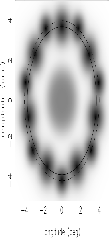
Figure 6: A gray scale representation of our rotating-subbeam model. Note the respective sets of PPM ($\parallel$ polarized) and SPM ($\perp$ polarized) “beamlets”, which in turn comprise the PPM (inner, solid) and SPM (outer, dashed) subcones. There is also an unpolarized, non-drifting central core component.

Figure 7: Simulated linear polarization histograms: (a) a conal double profile modeled on B0525+21, and (b) a conal single (“drifter”) profile modeled on P0820+02. See text for details. No effort has been made to model Stokes $V$ (dotted line). Pulsar names have been given as “0000+00”, just to indicate that the profiles are ‘simulated’.

As discussed earlier, conal component pairs exhibit large fractional linear polarization on their inner edges and pronounced (often nearly complete) depolarization on their outer edges. The three-way mode-segregation method provides some vital clues to understanding this phenomenon. The power corresponding to the weaker SPM is sufficient to dominate the PPM only on the outer “wings” of the profile.

The mode-segregation analyses above reveal two important characteristics of the emission beam configuration. First, the SPM emission is generally shifted further outward, away from the magnetic axis, than the PPM emission. If this modal radiation is emitted (in some average sense) by conal beams, then the emission conal region corresponding to the SPM beam must have a little larger radius than that of the PPM.

Second, as we saw in Fig. 5 the PPM and SPM power is substantially out of phase. Given the small $|\beta|/\rho$ for 1237+25—such that the sightline cuts the conal beams close to the magnetic axis—the phase difference suggests that emission elements within the respective modal beams are offset in magnetic azimuth! And, indeed, this is just the polarized-beam configuration observed in the rotating subbeam systems of conal single S_d pulsars B0809+74 (Rankin et al 2002) and 0943+10, where systematic longitude offsets between the modes (at $|\beta|/\rho\sim 1$) also indicate offsets in magnetic azimuth. In summary, the modal conal emission patterns are offset in both magnetic colatitude and azimuth.

We can begin to conceive, given the above observational indications, how complex are the modal depolarization dynamics of conal beams. The familiar polarization properties of conal component pairs are produced by central sightline trajectories (small $|\beta|/\rho$) and represent an angular average over the modal “beamlets”. For conal single (S_d) stars, however, the impact angle $|\beta|$ is very close to the radius of the emission cone $\rho$, and the observed average polarization will depend first on just how the sightline cuts the modal cones, and second on how this modal power is both angularly and temporally averaged.

In order to understand this situation more fully, we have attempted to simulate the depolarization processes in conal single and double pulsars. To do so, we generated an artificial pulsar signal such as would be detected by a pulsar backend connected to a radio telescope (e.g., WSRT with its PuMa processor). We computed this (partially) polarized signal using the recipe given in our Appendix, together with a rotating subbeam model interacting with a specific observer’s sightline. This subbeam system, with pairs of modal “beamlets” which could be offset in both magnetic colatitude $\rho$ and azimuth, flexibly modeled properties seen in both the S_d and D stars; and model pulses sequence were computed using relations very much like the inverse cartographic transform in Deshpande & Rankin (2001). Further, a low-level, non-drifting and unpolarized component, with a Gaussian-shaped pattern peaked along the magnetic axis, could be added to simulate weak core emission. Here, we have so far ignored the nature of the circular polarization but hope to address it in future work.

The modal “beamlet” pairs rotate rigidly with a period $\hat{P}_{3}$ around the magnetic axis, with their rotation phase “locked” to each other. Their respective trajectories have different radii (offset in magnetic azimuth), and the “beamlets” also have somewhat different radial widths. These characteristics are required in order both to permit high polarization on the inner edges of conal component pairs and to ensure that their outer edges are fully depolarized. In order to specify the radial illumination pattern of the modal “beamlets”, we have used a hybrid function with ranges of both Gaussian-like and exponential behavior,

$$P(\theta)\;=\;\frac{\exp[-\theta/2\sigma^{2}]+\exp[-\theta^{2}/2\sigma^{2}]}{1+\exp[-\theta^{2}/2\sigma^{2}]}$$ (1)

where $\theta$ is the radial distance from the centre of the “beamlet”, and $\sigma$ is its Gaussian-like rms scale. This functional form was chosen to provide a smoothly falling function near the “beamlet” peak and an exponential-like behavior on its edges. Although there is no physical basis for this choice, it seems to reproduce rather nicely the outer edges of the profiles shown in Fig. 1.

A schematic picture of our simulation model is then shown in Figure 6. Othogonally polarized sets of modal “beamlets” are shown in greyscale, which slowly rotate so as to form the two modal subcones. The peaks of the respective PPM ($\parallel$ polarization) and SPM ($\perp$ polarization) subcones are indicated by solid and dashed curves. A weak, non-drifting and unpolarized core beam is also included.

Figure 7 then shows some results from our simulations. The top panel represents an attempt to model a conal double (D) pulsar with properties similar to the canonical pulsar B0525+21. So, we have taken $\alpha$, $\beta$, and $P$ some 21^∘, 1.5^∘ and 3.75 s, respectively. Further, in order to model its 430-MHz profile, we took the mean radii of its two modal subbeam systems to be 3.0 and 3.6^∘. We also assumed that its two orthogonal modes are fully linearly polarised. The rotating-subbeam system corresponding to the PPM and SPM each have 8 subbeams, with $\sigma$ scales of 1.3^∘ and 0.88^∘ each, and the peak amplitudes of the SPM “beamlets” are about 60% of their PPM counterparts.

We also modeled the central core component [which for B0525+21 should have an observed width of 1.77^∘ (see Paper IV, eq. 5)] as a non-drifting, unpolarized pencil beam with a Gaussian profile centered along the magnetic axis. However, since our sightline intersects this weak emission far off on its beam edge ($\beta\sim$ 1.5 degrees), it contributes little to the model sequence and profile.

As can then be seen, the fractional linear polarization of the model profile reaches a maximum on the inner edges of the two components and drops sharply on their outer edges, just as is observed [c.f., Fig. 2 and, for instance, Blaskiewicz et al (1991)]. Note the ‘S’-shaped PA traverse and the parallel modal PA stripes on their outer edges, which correspond to those samples where the SPM sometimes dominates the PPM. This modal display is also usefully compared directly with the corresponding 430-MHz PA histogram of B0525+21 in Hankins, Rankin & Eilek (2002). Clearly, we have made no attempt to model the circular polarization.

The bottom panel of Fig. 7 then depicts our effort to simulate the polarized emission-beam configuration of a conal single (S_d) star, and here we have taken pulsar B0820+02 as an example. In this case we took $\alpha$, $\beta$, and $P$ some 19^∘, 5.5^∘ and 0.865 s, and the radii of the subcones corresponding to the PPM and SPM were 4.5^∘ and 5.1^∘, respectively—nearly equal to $|\beta|$ as expected. In this case, the weak unpolarized core beam has a computed with of 4.05^∘, and again contributes little to the model sequence and profile. Of course, we cannot know for S_d stars just how far out the sightline crosses the conal beam, so we can adjust this point slightly to match particular polarization characteristics.

The ratio of the two subcone radii in the respective examples chosen above are different. In the first case (B0525+21), it is 0.83 (3^∘/3.6^∘), while in the second case (B0820+02) 0.88. Although these two ratios are quite close in their values, it is unclear what might cause this ratio to vary from star to star. By contrast, within the dynamical picture we present here, the aggregate polarization properties must be independent of parameters such as $P_{2}$ (the subpulse separation in longitude), $P_{3}$ (the time for subpulse to drift through a longitudinal interval of $P_{2}$), and $\hat{P}_{3}$ (the subbeam circulation period). It is also important to note that the aggregate profile characteristics are completely independent of the total number of circulating subbeams.

In two particulars, our simulations depart significantly from what is observed: First, as a consequence of assuming that the modal emission is fully linearly polarized, we generally obtain higher levels of aggregate linear polarization than is seen in the profiles we are attempting to model. This suggests, as yet inconclusively, that the modal beams are not fully polarized. Second, we find much less scatter in the model PAs around the geometrically determined PA traverse. While the best observations have for some time suggested that this excessive scatter could not be the result of the system noise, more quantitative statements have not been easy to make. However, McKinnon & Stinebring (1998; 2000) have developed statistical analysis tools which should make a more meaningful assessment practical, and we plan to pursue this question in a future paper (Ramachandran & Rankin 2002).

Summary and Discussion

The results of this paper can be summarized succinctly: Conal beams have a rotating subbeam structure which also entails displacements between the PPM and SPM radiation in both magnetic latitude and azimuth. This results in the outer-edge depolarization seen in conal component pairs as well as the complex (and often nearly complete) depolarization found in pulsar profiles that represent an oblique sightline trajectory along the outer edge of the conal beam. It also provides a new and fundamental reason why the modal emission is so often statistically “disjoint” (see Cordes et al 1978). These characteristics of conal emission can be identified in a variety of ways, and the conclusions verified by detailed models and simulations.

It is also likely that these effects largely explain the frequency dependence of the fractional linear polarization in the classic cases of conal double profiles (i.e., B1133+16) first problematized by Manchester, Taylor & Huguenin (1973). Many more recent studies have pointed to both the the secular decline at high frequencies and the mid-band “break” point below which the aggregate fractional linear increases no further (e.g., McKinnon 1997). And closely associated with these profile effects are pulse-sequence phenomena ranging from the purported “randomizing” of the PA at high frequencies to distributions of polarization characteristics in subpulses. If we understand that the PPM and SPM “cones” have a significant displacement in magnetic colatitude at meter wavelengths, then radius-to-frequency mapping (see Paper VII) almost certainly tends to reduce this displacement at higher frequencies. Perhaps the characteristic depolarization of conal beams at very high frequencies (as well as the “random” PAs) is simply the result of modal beam overlap. Perhaps the “breaks” mark the frequency at which the modal beams diverge to the point that no further depolarization occurs. It will be satisfying to test these ideas in future detailed studies.

The origin of “orthogonal mode” emission has been a topic of debate for decades. Numerous models have been suggested wherein the two modes are intrinsic to the emission mechanism itself (e.g., Gangadhara 1997) and, lacking strong contrary evidence, some bias has developed in favor of this assumption. However, direct production implies that the modes be fully (elliptically) polarized and associates them with a basic emission mechanism which is itself still unknown [for a review, see Melrose (1995)].

The possibility that disjoint orthogonal modes can arise from propagation effects was also explored very early by several authors (Melrose 1979; Allan & Melrose 1982). The central idea here is that the natural wave modes, being linearly polarized in two orthogonal planes, have different refractive indices, and become separated in space and angle during their propagation. This phenomenon of refraction in the magnetosphere was explored rigorously by Barnard & Arons (1986).

A recent work of Petrova (2001) has addressed these issues in greater detail. According to her model, the primary pulsar radiation is comprised of only one (ordinary) mode, which is later partially converted into extraordinary-mode emission. It is in this conversion that the orthogonal polarization modes arise. Therefore, the transition from one mode to the other, as observed in pulsar emission, can be understood as due to switching between a “significant” and “insignificant” conversion. At any given time and pulse longitude, the disjoint mode is the sum of two incoherently superposed modes. This nicely explains the partial polarization observed in the pulsar radiation.

Conversion to the extraordinary mode, in Petrova’s model, is easiest for those rays which are refracted outward, away from the magnetic axis, and such emission apparently comprises the conal beam—though her work yet gives no understanding about why there should be two distinct types of conal beams that are both present in some cases. It is further unclear how the ordinary or extraordinary mode would be polarized, thus how it then could be identified as a specific PPM or SPM in a given pulsar, and why one or the other should experience a greater angular offset in magnetic colatitude. Finally, this model appears to be fully symmetric in azimuth, so that it is again hard to see how the wave-propagation effects can explain the observed angular offsets in magnetic azimuth.

To summarise, the important conclusions of this work are as follows:

• The average profiles of pulsars with conal component pairs exhibit low fractional polarization on their outer edges, and often high fractional linear polarization on their inner edges.

• This very general behavior can be understood in terms of the dynamic averaging, along the observer’s sightline, of emission from a rotating system of subbeams with systematic modal offsets.

• The “beamlet” pairs corresponding to the PPM and SPM emission are offset not only in magnetic latitude, but also in magnetic longitude. In other words, the respective average modal beams can be visualized as distinct emission cones with somewhat different angular radii. Dynamically, the “beamlet” pairs maintain a fixed relation to each other as they circulate about the magnetic axis.

• The outer-edge depolarization requires that the PPM and SPM subcones have nearly identical specific intensity and angular dependence in this region. This would appear to place strong constraints on their physical origin.

• The causes of these remarkable angular offsets between the PPM and SPM emission is unclear. Propagation effects can more easily explain the shifts in magnetic latitude than longitude.

Appendix: Simulation of Partially Polarized Radiation

Let us consider the two complex signals, $X(t)\,=\,[X_{R}(t)\,+\,j\,X_{I}(t)]$ and $Y(t)\,=\,[Y_{R}(t)\,+\,j\,Y_{I}(t)]$, which represent the Nyquist-sampled baseband voltages from the two orthogonal linear dipoles (X & Y) of a radio telescope. The subscripts $R$ and $I$ indicate the real and the imaginary parts of the complex signal, and $j\;=\;\sqrt{-1}$. The Stokes parameters are defined as

$$I = \langle X\;X^{\star}\;+\;Y\;Y^{\star}\rangle$$

$$Q = \langle X\;X^{\star}\;-\;Y\;Y^{\star}\rangle$$

$$U = \langle{\tt Re}[X\;Y^{\star}\;+\;X^{\star}\;Y]\rangle$$

$$= \langle 2\;|X|\;|Y|\;\cos\theta(t)\rangle$$

$$V = \langle{\tt Im}[X\;Y^{\star}\;+\;X^{\star}\;Y]\rangle$$ (2)

$$= \langle 2\;|X|\;|Y|\;\sin\theta(t)\rangle$$

The $\langle$ $\rangle$ symbols indicate time-averaging, Re and Im the real and imaginary parts, and superscript “$\star$” the complex conjugate. $Q$ and $U$ describe the linear and $V$ the circular polarization, obeying the well known inequality, $I\geq\sqrt{Q^{2}+U^{2}+V^{2}}$. The angle $\theta$ is the phase between $X(t)$ and $Y(t)$, which is given by $\theta\,=\,[\tan^{-1}(X_{I}/X_{R})\;-\;\tan^{-1}(Y_{I}/Y_{R})]$.

From the sampling theorem, we know that a signal varies at a rate given by the reciprocal of the bandwidth $\Delta\nu$; samples having this resolution are fully polarized and can be represented by a point on the Poinćare sphere. Polarimetry, then, always entails averaging over a time sufficient to adequately reduce the statistical errors.

To generate a realistic partially polarized Nyquist-sampled baseband signal, we adopted the following procedure. A randomly polarized voltage sample in the X-dipole was defined as

$$X_{Ru}^{i} = \sqrt{1/2}\;P_{r}\;G_{x}^{i}\;\cos(\phi)$$

$$X_{Iu}^{i} = \sqrt{1/2}\;P_{r}\;G_{x}^{i}\;\sin(\phi)$$

$${\rm where}\;\;\;\phi = 2\pi\;U_{x}^{i}\ ,$$ (3)

where $P_{r}$ is its amplitude, $G_{x}^{i}$ is a Gaussian-distributed random variable with zero mean and unity rms amplitude, and $U_{x}^{i}$ a uniform random variable with equal density between 0 and 1. Similarly, for the Y-dipole,

$$Y_{Ru}^{i} = \sqrt{1/2}\;P_{r}\;G_{y}^{i}\;\cos(\phi)$$

$$Y_{Iu}^{i} = \sqrt{1/2}\;P_{r}\;G_{y}^{i}\;\sin(\phi)$$

$${\rm where}\;\;\;\phi = 2\pi\;U_{y}^{i}\ ,$$ (4)

and $G_{y}^{i}$, $U_{y}^{i}$ are different random variables as above.

For linear polarization, the signal voltages are

$$X_{Rl}^{i} = \cos\chi\;P_{l}\;G_{l}^{i}\;\cos(\phi)$$

$$X_{Rl}^{i} = \cos\chi\;P_{l}\;G_{l}^{i}\;\sin(\phi)$$

$$Y_{Rl}^{i} = \sin\chi\;P_{l}\;G_{l}^{i}\;\cos(\phi)$$

$$Y_{Rl}^{i} = \sin\chi\;P_{l}\;G_{l}^{i}\;\sin(\phi)$$

$${\rm where}\;\;\;\phi = 2\pi\;U_{l}^{i}\ ,$$ (5)

and for circular polarization they are

$$X_{Rc}^{i} = \sqrt{1/2}\;P_{c}\;G_{c}^{i}\;\cos(\phi)$$

$$X_{Ic}^{i} = \sqrt{1/2}\;P_{c}\;G_{c}^{i}\;\sin(\phi)$$

$$Y_{Rc}^{i} = -\;\sqrt{1/2}\;P_{c}\;G_{c}^{i}\;\sin(\phi)$$

$$Y_{Ic}^{i} = +\sqrt{1/2}\;P_{c}\;G_{c}^{i}\;\cos(\phi)$$

$${\rm where}\;\;\;\phi = 2\pi\;U_{l}^{i}\ ,$$ (6)

and, $G_{l}^{i}$, $U_{l}^{i}$, $G_{c}^{i}$, $U_{c}^{i}$ are other random variables as above.

The partially polarized observed voltage corresponding to a given sample is then

$$X_{R}^{i} = \left[X_{Rr}^{i}\;+\;X_{Rl}^{i}\;+\;X_{Rc}^{i}\right]$$

$$X_{I}^{i} = \left[X_{Ir}^{i}\;+\;X_{Il}^{i}\;+\;X_{Ic}^{i}\right]$$

$$Y_{R}^{i} = \left[Y_{Rr}^{i}\;+\;Y_{Rl}^{i}\;+\;Y_{Rc}^{i}\right]$$

$$Y_{I}^{i} = \left[Y_{Ir}^{i}\;+\;Y_{Il}^{i}\;+\;Y_{Ic}^{i}\right]\ ,$$ (7)

and the Stokes parameters corresponding to this sample are computed according to Eqn. 2. These Stokes-parameters samples are averaged over $N$ samples to achieve a desired resolution and statistical significance in the simulated time series.

References

- Allan & Melrose (1982) Allan, M. C., & Melrose, D. B. 1982, Proc. Astron. Soc. Australia, 4, 365.
- Backer (1973) Backer, D. C 1973, ApJ, 182, 245
- Backer et al (1975) Backer, D. C., Rankin, J. M., & Campbell, D. B. 1975, ApJ, 197, 481.
- Barnard & Arons, J. (1986) Barnard, J. J., & Arons, J. ApJ, 320, 138
- Bartel et al (1981) Bartel, N., Kardeshev, N. S., Kuzmin, A. D., Nikolaev, N. Ya., Popov, M. V., Sieber, W., Smirnova, T. V., Soglasnov, V. A., & Wielebinski, R. 1981, A&A, 93, 85.
- Bartel (1981) Bartel, N. 1981, A&A, 97, 384.
- Bartel et al (1982) Bartel, N., Morris, D., Sieber, W., & Hankins, T. H. 1982, ApJ, 258, 776
- Blaskiewicz et al (1991) Blaskiewicz, M., Cordes, J. M., & Wasserman, I. 1991, ApJ, 370, 643 (BCW)
- Cordes, Rankin & Backer (1978) Cordes, J. M., Rankin, J. M. & Backer, D. C. 1978, ApJ, 223, 961.
- Deshpande & Rankin (1999) Deshpande, A. A. & Rankin, J. M. 1999, ApJ, 524, 1008
- Deshpande & Rankin (2001) Deshpande, A. A. & Rankin, J. M. 2001, MNRAS, 322, 438
- Everett, & Weisberg (2001) Everett, J. E. & Weisberg J. M. 2001, ApJ, 553, 341.
- Gangadhara (1997) Gangadhara, R. T. 1997, A&A, 327, 155.
- Gil & Lyne (1995) Gil, J. & Lyne, A. G. 1995, MNRAS, 276, L55
- Gould & Lyne (1998) Gould, D. M. & Lyne, A. G. 1998, MNRAS, 301, 235.
- Hankins, Rankin, & Eilek (2001) Hankins, T. H., Rankin, J. M., & Eilek, J. A., 2002, in preparation
- von Hoensbroech (1999) von Hoensbroech, A., 1999, Ph.D. Thesis, Max Planck Institut für Radioastronomie, Bonn
- von Hoensbroech & Xilouris (1997a) von Hoensbroech, A., & Xilouris, K. M. 1997a, A&AS, 126, 121
- von Hoensbroech & Xilouris (1997b) von Hoensbroech, A., & Xilouris, K. M. 1997b, A&A, 324, 981
- Manchester (1971) Manchester, R. N. 1971, ApJS, 23, 283.
- Manchester, Taylor & Huguenin (1973) Manchester, R. N., Taylor, J. H., & Huguenin, G. R. 1973, ApJ, 179, L7.
- Melrose (1979) Melrose, D. B. 1979, Australian Journal of Physics, 32, 61.
- Melrose (1995) Melrose, D. B. 1995, J. Astrophys. & Astronomy, 16, 137
- Manchester et al. (1975) Manchester, R. N., Taylor, J. H., & Huguenin, G. R. 1975, ApJ, 196, 83.
- McKinnon (1997) McKinnon, M. M. 1997 ApJ, 475, 763.
- McKinnon, & Stinebring (1998) McKinnon, M. M., & Stinebring, D. R. 1998 ApJ, 502, 883.
- McKinnon, & Stinebring (2000) McKinnon, M. M., & Stinebring, D. R. 2000 ApJ, 529, 435.
- Mitra (1999) Mitra, D. 1999, Ph.D. Thesis, Raman Research Institute, Bangalore
- Mitra & Rankin (2002) Mitra, D., & Rankin, J. M. 2002, ApJ, in press (Paper VII)
- Morris et al (1981) Morris, D., Graham, D. A., Sieber, W., Bartel, N., & Thomasson, P. 1981, A&AS, 46, 42.
- Petrova (2001) Petrova, S. A. 2001, A&A, 378, 883.
- Radhakrishnan & Cooke (1969) Radhakrishnan, V., & Cooke, D. J. 1969, Astrophys. Lett., 3, 225
- Radhakrishnan & Rankin (1990) Radhakrishnan, V. & Rankin, J. M. 1990, ApJ, 352, 258 (Paper V)
- Ramachandran et al. (2002) Ramachandran, R., Rankin, J. M., Stappers, B. W., Kouwenhoven, M. L. A., & van Leeuwen, A. G. J. 2002, A&A, 381, 993
- Rankin (1983a) Rankin, J. M. 1983a, ApJ, 274, 333 (Paper I)
- Rankin (1983b) Rankin, J. M. 1983b, ApJ, 274, 359 (Paper II)
- Rankin (1986) Rankin, J. M. 1986, ApJ, 301, 901 (Paper III)
- Rankin (1990) Rankin, J. M. 1990, ApJ, 352, 247 (Paper IV)
- Rankin (1993a) Rankin, J. M. 1993a, ApJ, 405, 285 (Paper VIa)
- Rankin (1993b) Rankin, J. M. 1993b, ApJS, 85, 145 (Paper VIb)
- Rankin, Ramachandran, & van Leeuwen (2002) Rankin, J. M., Ramachandran, R., & van Leeuwen, A. G. J. 2002, A&A, preprint.
- Rankin & Rathnasree (1997) Rankin, J. M., & Rathnasree, N. 1997, JAA, 18, 91.
- Ruderman & Sutherland (1975) Ruderman, M. A., & Sutherland, P. G. 1975, ApJ, 196, 51
- Ruderman (1976) Ruderman, M. A. 1976, ApJ, 203, 206
- Sieber & Oster (1975) Sieber, W., & Oster, L. 1975, A&A, 38, 325
- Sieber & Oster (1976) Sieber, W., & Oster, L. 1976, ApJ, 210, 220
- Suleymanova & Izvekova (1984) Suleymanova, S. A., & Izvekova, V. A. 1984, Soviet Astronomy, 28, 32
- Suleymanova et al. (1998) Suleymanova, S. A., Izvekova, V. A., Rankin, J. M. & Rathnasree, N. 1998, J. Astrophys. Astron., 19, 1
- Suleymanova & Pugachev (1998) Suleymanova, S. A., & Pugachev, V. D. 1998, Astronomy Reports, 42, 252.
- Suleymanova & Pugachev (2002) Suleymanova, S. A., & Pugachev, V. D. 2002, Astronomy Reports, 46, 34.
- Taylor & Cordes (1993) Taylor, J. H. & Cordes, J. M. 1993, ApJ, 401, 674
- Taylor & Huguenin (1971) Taylor, J. H., & Huguenin, G. R. 1971, ApJ, 167, 273
- Taylor et al. (1971) Taylor, J. H., Huguenin, G. R., Hirsch, R. M., & Manchester, R. N. 1971, Astrophys. Lett., 9, 205
- Taylor et al. (1993) Taylor, J. H., Manchester, R. N., & Lyne, A. G. 1993, ApJS, 88, 529
- Weisberg et al (1999) Weisberg, J. M., Cordes, J. M., Lundgren, S. C., Dawson, B. R., Despotes, J. T., Morgan, J. J., Weitz, K. A., Zink, E. C. & Backer, D. C., 1999, ApJS, 121, 171