Energy, momentum and angular momentum radiation from chiral cosmic string loops

Abstract

We derived expressions for energy, momentum and angular momentum losses due to gravitational and electromagnetic radiation from the closed superconducting chiral cosmic strings of arbitrary form. The expressions for corresponding radiation rates into the unit solid angle have the form of four-dimensional integrals. In the special case of piece-wise linear strings these formulas are reduced to sums over the kinks. We calculate numerically the total radiation rates for three examples of string loops in dependence of current along the string.

,

1 Introduction

We study the gravitational and electromagnetic radiation of energy, momentum and angular momentum of superconducting closed cosmic strings with chiral current. Cosmic strings are linear topological defects, that may have been created during phase transitions in the early Universe (see e. g. reviews in [1, 2]). Oscillating ordinary cosmic strings (without current) radiate only gravitational waves. The corresponding energy radiation was studied in [3, 4, 5, 6, 7, 8]. Besides energy, gravitational waves from strings take also momentum [3, 9, 10] and angular momentum [10]. It was found that the rates (averaged per oscillation period) of energy $\dot{E}$, momentum $\dot{P}$ and angular momentum $\dot{L}$ losses can be expressed in the following form: $\dot{E}^{\rm{gr}}=\Gamma_{E}^{\rm{gr}}G\mu^{2}$, $\dot{P}^{\rm{gr}}=\Gamma_{P}^{\rm{gr}}G\mu^{2}$, $\dot{L}^{\rm{gr}}=\Gamma_{L}^{\rm{gr}}\mathcal{L}G\mu^{2}$, where $\Gamma_{E}^{\rm{gr}}\sim 100$, $\Gamma_{P}^{\rm{gr}}\sim 10$ and $\Gamma_{L}^{\rm{gr}}\sim 10$ are numerical coefficients, depending on the particular string configuration, $\mathcal{L}$ is length of the string, $\mu$ is string mass per unit length and used units $\hbar=c=1$.

Witten [11] showed that in some field theory models the cosmic strings can carry superconducting current which is coupled to some gauge field. In the case of electromagnetic gauge field the superconducting cosmic string loops would radiate not only gravitational waves, but also electromagnetic ones. Equations of motion of superconducting cosmic strings can be solved analytically [12, 13, 14] if (i) the influence of gauge field on the string motion is negligible and (ii) the current on the string $j^{\mu}$ is chiral, i. e. $j^{\mu}j_{\mu}=0$. The gravitational and electromagnetic energy radiated by the single cusp on chiral cosmic string was studied by Blanco-Pillado and Olum [15] in the case of small current. The opposite case for current which is close to maximum value was considered in [16]. If the string carries the current, then the coefficients $\Gamma_{E}^{\rm{gr}}$, $\Gamma_{P}^{\rm{gr}}$ and $\Gamma_{L}^{\rm{gr}}$ which determine the gravitational radiation depend on the current along the string. Corresponding expressions for electromagnetic radiation have the similar form: $\dot{E}^{\rm{em}}=\Gamma_{E}^{\rm{em}}\mu q^{2}$, $\dot{P}^{\rm{em}}=\Gamma_{P}^{\rm{em}}\mu q^{2}$, $\dot{L}^{\rm{em}}=\Gamma_{L}^{\rm{em}}\mathcal{L}\mu q^{2}$, where numerical coefficients $\Gamma_{E}^{\rm{em}}$, $\Gamma_{P}^{\rm{em}}$ and $\Gamma_{L}^{\rm{em}}$ also depend on the current on the string.

In this paper we present the results for gravitational and electromagnetic radiation of energy, momentum and angular momentum from chiral cosmic string loops for any value of superconducting current. Due to the periodic motion of the cosmic string loops the rates of radiation losses can be expand in series $\dot{E}=\sum\dot{E}_{l}$, $\dot{P}=\sum\dot{P}_{l}$, $\dot{L}=\sum\dot{L}_{l}$. Here $\dot{E}_{l}$, $\dot{P}_{l}$ and $\dot{L}_{l}$ are correspondingly the energy, momentum and angular momentum rates in the $l$-th radiation mode. Usually the total rates per unit time (averaged over the period) are calculated by summing of losses in different modes. In practical numerical calculations the values of $\dot{E}$, $\dot{P}$ and $\dot{L}$ are determined with the accuracy up to the $l$ of a few hundred. Such calculations may be not correct because of the slow convergence of the corresponding sums over $l$ as was pointed out by Allen et al. [7]. See however [7, 8, 9] where for some special cases of ordinary string loops the summation over $l$ was done and analytic expressions for the total energy and momentum rates into gravitational waves were obtained. We perform in the following the summation over radiation modes analytically and derive the formulas for energy, momentum and angular momentum rates into the both the gravitational and electromagnetic radiation from chiral string loops of general configuration. The corresponding radiation rates into the unit solid angle are reduced to the four-dimensional integrals which in general case can be calculated only numerically. For chiral piece-wise linear loops these formulas lead to analytic expressions for the energy, momentum and angular momentum radiation into the unit solid angle.

We considered three examples of chiral string loops and calculated the total radiated energy, moment and angular moment per unit time in dependence of current on the string. The first and the second examples are piece-wise linear loops (or ”kinky” loops), and the third example is a hybrid of piece-wise loop and smooth loop (namely, the $a$-loop is smooth and $b$-loop is piece-wise loop). Unfortunately we are unable to present the results for kinkless cosmic loops (i. e. for smooth $a$ and $b$-loops), because it would take an enormous amount of computer time.

The paper is organized as follows. In Section 2 we review some general properties of chiral cosmic strings. In Section 3 we derive new expressions for gravitational radiation rates of energy, momentum and angular momentum by chiral loops of general configuration into the unit solid angle. These expressions are reduced to the four-dimensional integrals where the summation over all radiation modes were performed analytically. In Section 4 we derive the similar formulas for electromagnetic radiation rates. In Section 5 we present numerical calculations of electromagnetic and gravitational radiation rates for some illustrative examples of chiral loops and study the properties of chiral strings radiation in dependence of current. In conclusion Section 6 we describe the obtained results and discuss some qualitative features of gravitational and electromagnetic radiation from chiral loops.

2 Chiral string motion in flat space-time

While moving cosmic string sweeps out a two-dimensional world-sheet in the Minkowskian space-time. The four-dimensional coordinates of string are functions of two world-sheet parameters $x^{\mu}=x^{\mu}(\sigma^{a})$, where indexes $a$ take values $0$, $1$ and $\sigma^{a}$ are correspondingly the coordinates on a two-dimensional world-sheet. The convenient gauge choice is such that $\sigma^{0}$ is the Minkowskian time $t$ and $\sigma^{1}$ parameterizes the string total energy:

$$E=\mu\int d\sigma.$$ (1)

In this gauge the general solution of the equations of motion of the chiral string is [12, 13, 14]:

$$x^{0}=t,\quad\mathbf{x}(t,\sigma)=\frac{\mathcal{L}}{4\pi}\left[\mathbf{a}(\xi)+\mathbf{b}(\eta)\right],$$ (2)

where ${\mathcal{L}}$ is the invariant length of the string, $\mathbf{a}(\xi)$ and $\mathbf{b}(\eta)$ are arbitrary vector functions of $\xi=(2\pi/{\mathcal{L}})(\sigma-t)$ and $\eta=(2\pi/{\mathcal{L}})(\sigma+t)$ obeying the following conditions:

$${\mathbf{a}^{\prime}}^{2}=1,\quad{\mathbf{b}^{\prime}}^{2}=k^{2}(\eta)\leq 1.$$ (3)

In the case of closed chiral strings (loops) the vector functions $\mathbf{a}(\xi)$ and $\mathbf{b}(\eta)$ form closed loops, called $a$- and $b$- loops. The function $k(\eta)$ in (3) may be expressed as follows [14]:

$$k^{2}(\eta)=1-\frac{4F^{\prime 2}(\eta)}{\mu},$$ (4)

where function $F(\eta)$ defines in turn the auxiliary scalar field

$$\phi(\sigma,t)=\frac{\mathcal{L}}{2\pi}F(\eta).$$ (5)

According to (5) the scalar field $\phi(\sigma,t)$ is an arbitrary function of the only parameter $\eta$. The four-dimensional current on the string is expressed through this scalar field $\phi(\sigma,t)$ in the following way [20]:

$$j^{\mu}(\mathbf{x},t)=q\int d\sigma\phi^{\prime}(\sigma,t)(x^{\prime\mu}-\dot{x}^{\mu})\delta^{(3)}\left(\mathbf{x}-\mathbf{x}(\sigma,t)\right),$$ (6)

where $x^{\prime}$ denotes $\partial x/\partial\sigma$ and $\dot{x}$ denotes $\partial x/\partial t$. The energy-momentum tensor of the string in this gauge is

$$T^{\mu\nu}=\mu\int d\sigma\left(\dot{x}^{\mu}\dot{x}^{\nu}-x^{\prime\mu}x^{\prime\nu}\right)\delta^{(3)}\left(\mathbf{x}-\mathbf{x}(\sigma,t)\right).$$ (7)

Correspondingly the total momentum and angular momentum of the string are

$$\mathbf{P}=\mu\int d\sigma\dot{\mathbf{x}}(\sigma,t),$$ (8)

$$\mathbf{L}=\mu\int d\sigma\mathbf{x}(\sigma,t)\times\dot{\mathbf{x}}(\sigma,t).$$ (9)

3 Gravitational radiation from chiral loops

Let us consider the periodic system with period $T$. The Fourier transform of energy-momentum tensor of this system $T^{\mu\nu}(\mathbf{x},t)$ can be given by [10]:

$$\hat{T}^{\mu\nu}(\omega_{l},\mathbf{n})=\frac{1}{T}\int_{0}^{T}dt\int d^{3}xT^{\mu\nu}(\mathbf{x},t)e^{i\omega_{l}(t-\mathbf{n}\mathbf{x})},$$ (10)

where $\omega_{l}=2\pi l/T$ and $\mathbf{n}$ is an arbitrary unit vector. It is useful to define also the Fourier transform of the first moment:

$$\hat{T}^{\mu\nu p}(\omega_{l},\mathbf{n})=\frac{1}{T}\int dt\int d^{3}xT^{\mu\nu}(\mathbf{x},t)x^{p}e^{i\omega_{l}(t-\mathbf{n}\mathbf{x})}.$$ (11)

Let us further define for convenience the four-dimensional symbol $n^{\mu}\equiv(1,\mathbf{n})$. For any periodic system the corresponding gravitational energy, momentum and angular momentum radiation rates (averaged over the period $T$) per solid angle $d\Omega$ is given by series

$$\frac{d\dot{P}^{\mu}}{d\Omega}=\sum_{n=1}^{\infty}\frac{d\dot{{P}^{\mu}}({\omega}_{n})}{d\Omega},\quad\frac{d\dot{\mathbf{L}}}{d\Omega}=\sum_{n=1}^{\infty}\frac{d\dot{\mathbf{L}}({\omega}_{n})}{d\Omega},$$ (12)

where [17]

$$\frac{d\dot{P}^{\mu}(\omega)}{d\Omega}=-n^{\mu}\frac{G\omega^{2}}{\pi}P_{ij}P_{lm}[\hat{T}^{*}_{il}\hat{T}_{jm}-\frac{1}{2}\hat{T}^{*}_{ij}\hat{T}_{lm}]$$ (13)

and [10]

$$\frac{d\dot{L}_{i}(\omega)}{d\Omega} =-\frac{G}{2\pi}\epsilon^{ijk}n^{j}\left[i\omega n^{l}P^{pq}(3\hat{T}^{*}_{kl}\hat{T}_{qp}+6\hat{T}^{*}_{kp}\hat{T}_{ql})\right.$$ (14)

$$+ \!\!\!\!\!\!\!\left.\omega^{2}P^{lm}P^{pq}(2\hat{T}^{*}_{kmq}\hat{T}_{lp}-2\hat{T}^{*}_{km}\hat{T}_{lpq}-\hat{T}^{*}_{lpk}\hat{T}_{mq}+\frac{1}{2}\hat{T}^{*}_{lmk}\hat{T}_{pq})+c.c\right].$$

Here $P_{ij}=\delta_{ij}-n_{i}n_{j}$ is the projection operator to the plane perpendicular to the unit vector $\mathbf{n}$. It is possible to simplify (13) and (14) further by rewriting them in the corotating basis $(\mathbf{e}_{1},\mathbf{e}_{2},\mathbf{e}_{3})\equiv(\mathbf{n},\mathbf{v},\mathbf{w})$, where $\mathbf{v}$ and $\mathbf{w}$ are the arbitrary unit vectors, perpendicular each other and to vector $\mathbf{n}$. In this corotating basis (13) and (14) transform to the form [10]:

$$\frac{d\dot{P^{\mu}}({\omega})}{d\Omega}=n^{\mu}\frac{G{\omega}^{2}}{\pi}[{\tau}^{*}_{pq}{\tau}_{pq}-\frac{1}{2}{\tau}^{*}_{qq}{\tau}_{pp}],$$ (15)

$$\frac{d\dot{\mathbf{L}}({\omega})}{d\Omega}=\frac{d\dot{L}_{2}}{d\Omega}\mathbf{v}+\frac{d\dot{L}_{3}}{d\Omega}\mathbf{w},$$ (16)

where

$$\frac{d\dot{L}_{2}}{d\Omega} = \frac{G}{2\pi}[-i\omega(3{\tau}^{*}_{13}{\tau}_{pp}+6{\tau}^{*}_{3p}{\tau}_{p1})$$

$$- {\omega}^{2}(2{\tau}^{*}_{3pq}{\tau}_{pq}-2{\tau}^{*}_{3p}{\tau}_{pqq}-{\tau}^{*}_{pq3}{\tau}_{pq}+\frac{1}{2}{\tau}^{*}_{qq3}{\tau}_{pp})+c.c],$$

$$\frac{d\dot{L}_{3}}{d\Omega} = \frac{G}{2\pi}[i\omega(3{\tau}^{*}_{12}{\tau}_{pp}+6{\tau}^{*}_{2p}{\tau}_{p1})$$ (17)

$$+ {\omega}^{2}(2{\tau}^{*}_{2pq}{\tau}_{pq}-2{\tau}^{*}_{2p}{\tau}_{pqq}-{\tau}^{*}_{pq2}{\tau}_{pq}+\frac{1}{2}{\tau}^{*}_{qq2}{\tau}_{pp})+c.c].$$

Here $\tau_{pq}$ and $\tau_{pqr}$ are correspondingly Fourier-transforms of an energy-momentum tensor and its first moment in new the corotating basis. Note that only indexes $p,q$ with values $2$ and $3$ appear in the equations (15) and (3). Fourier-transforms $\tau_{pq}$ for chiral loops can be expressed in the following way:

$${\tau}_{pq}(\omega_{l},\mathbf{n})=-\frac{{\mathcal{L}}\mu}{2}[I_{p}(l)Y_{q}(l)+Y_{p}(l)I_{q}(l)],$$ (18)

where functions $I_{p}(l)$ and $Y_{q}(l)$ are expressed through the “fundamental integrals”:

$$I_{i}(l) \equiv \frac{1}{2\pi}\int_{0}^{2\pi}d\xi e^{-il[\xi+\mathbf{n}\mathbf{a}(\xi)]}\mathbf{a}^{\prime}(\xi)\mathbf{e_{i}},$$

$$Y_{j}(l) \equiv \frac{1}{2\pi}\int_{0}^{2\pi}d\eta e^{il[\eta-\mathbf{n}\mathbf{b}(\eta)]}\mathbf{b}^{\prime}(\eta)\mathbf{e_{j}}.$$ (19)

Similarly for the first moment (11) one can find:

$${\tau}_{ijk} (\omega_{l},\mathbf{n})=$$ (20)

$$- \frac{\mathcal{L}^{2}\mu}{8\pi}[I_{i}(l)N_{jk}(l)+I_{j}(l)N_{ik}(l)+Y_{i}(l)M_{jk}(l)+Y_{j}(l)M_{ik}(l)],$$

where

$$M_{ij}(l) \equiv \frac{1}{2\pi}\int_{0}^{2\pi}d\xi e^{-il[\xi+\mathbf{n}\mathbf{a}(\xi)]}\,(\mathbf{a}^{\prime}(\xi)\mathbf{e_{i}})\,(\mathbf{a}(\xi)\mathbf{e_{j}}),$$

$$N_{ij}(l) \equiv \frac{1}{2\pi}\int_{0}^{2\pi}d\eta e^{il[\eta-\mathbf{n}\mathbf{b}(\eta)]}\,(\mathbf{b}^{\prime}(\eta)\mathbf{e_{i}})\,(\mathbf{b}(\eta)\mathbf{e_{j}}).$$ (21)

The crucial point of our following calculations is the summations over the all mode numbers $l$ in expressions (12) for the requested rates of radiated gravitational energy, momentum and angular momentum. To do this we first integrate expressions (3) and (3) in parts to get additional $l$ in the denominator. For example for function $I_{i}$ we have:

$$I_{i}(l) = \frac{1}{2\pi}\int_{0}^{2\pi}d\xi\left[e^{-il(\xi+\mathbf{n}\mathbf{a})}(1+\mathbf{n}\mathbf{a^{\prime}})\right]\frac{\mathbf{a}^{\prime}\mathbf{e_{i}}}{1+\mathbf{n}\mathbf{a^{\prime}}}=$$ (22)

$$- \frac{1}{2\pi il}\frac{\mathbf{a}^{\prime}\mathbf{e_{i}}}{1+\mathbf{n}\mathbf{a^{\prime}}}e^{-il(\xi+\mathbf{n}\mathbf{a})}\Big{|}_{0}^{2\pi}+\frac{1}{2\pi il}\int_{0}^{2\pi}d\xi\,\left[\frac{\mathbf{a^{\prime}}\mathbf{e_{j}}}{1+\mathbf{n}\mathbf{a^{\prime}}}\right]^{\prime}e^{-il(\xi+\mathbf{n}\mathbf{a})}.$$

The first term in last expression turns to zero because of the periodicity of $a$- and $b$- loops. In a similar way the expressions for functions $Y_{j}$, $M_{ij}$ and $M_{ij}$ can be integrated by parts. Finally we obtain:

$$I_{i} = \frac{1}{2\pi il}\int_{0}^{2\pi}d\xi\,\mathcal{I}_{i}e^{-il(\xi+\mathbf{n}\mathbf{a})},\quad Y_{j}=-\frac{1}{2\pi il}\int_{0}^{2\pi}d\eta\,\mathcal{Y}_{j}e^{il(\eta-\mathbf{n}\mathbf{b})},$$

$$M_{ij} = \int_{0}^{2\pi}d\xi\left(\frac{1}{2\pi il}\mathcal{M}_{ij}-\frac{1}{2\pi l^{2}}\tilde{\mathcal{M}}_{ij}\right)e^{-il(\xi+\mathbf{n}\mathbf{a})},$$ (23)

$$N_{ij} = -\int_{0}^{2\pi}d\eta\left(\frac{1}{2\pi il}\mathcal{N}_{ij}+\frac{1}{2\pi l^{2}}\tilde{\mathcal{N}}_{ij}\right)e^{il(\eta-\mathbf{n}\mathbf{b})},$$

where

$$\mathcal{I}_{i} = \left[\frac{\mathbf{a^{\prime}}\mathbf{e_{i}}}{1+\mathbf{n}\mathbf{a^{\prime}}}\right]^{\prime},\quad\mathcal{Y}_{j}=\left[\frac{\mathbf{b^{\prime}}\mathbf{e_{j}}}{1-\mathbf{n}\mathbf{b^{\prime}}}\right]^{\prime},$$

$$\mathcal{M}_{ij} = \left[\frac{\mathbf{a^{\prime}}\mathbf{e_{i}}}{1+\mathbf{n}\mathbf{a^{\prime}}}\right]^{\prime}(\mathbf{a}\mathbf{e_{j}}),\quad\tilde{\mathcal{M}}_{ij}=\left[\frac{(\mathbf{a^{\prime}}\mathbf{e_{i}})(\mathbf{a^{\prime}}\mathbf{e_{j}})}{(1+\mathbf{n}\mathbf{a^{\prime}})^{2}}\right]^{\prime},$$ (24)

$$\mathcal{N}_{ij} = \left[\frac{\mathbf{b^{\prime}}\mathbf{e_{i}}}{1-\mathbf{n}\mathbf{b^{\prime}}}\right]^{\prime}(\mathbf{b}\mathbf{e_{j}}),\quad\tilde{\mathcal{N}}_{ij}=\left[\frac{(\mathbf{b^{\prime}}\mathbf{e_{i}})(\mathbf{b^{\prime}}\mathbf{e_{j}})}{(1-\mathbf{n}\mathbf{b^{\prime}})^{2}}\right]^{\prime}.$$

Substituting (3) into (18) and (20) we find:

$$\tau_{ij} = -\frac{{\mathcal{L}}\mu}{8\pi^{2}l^{2}}\int_{0}^{2\pi}\int_{0}^{2\pi}d\xi d\eta\,\mathcal{T}_{ij}\,e^{-il[\xi-\eta+\mathbf{n}(\mathbf{a}(\xi)+\mathbf{b}(\eta))]},$$

$$\tau_{ijk} = -\frac{{\mathcal{L}^{2}}\mu}{32\pi^{3}l^{2}}\int_{0}^{2\pi}\int_{0}^{2\pi}d\xi d\eta\,\left(\mathcal{T}_{ijk}+\frac{1}{il}\tilde{\mathcal{T}}_{ijk}\right)\,e^{-il[\xi-\eta+\mathbf{n}(\mathbf{a}(\xi)+\mathbf{b}(\eta))]},$$ (25)

where

$$\mathcal{T}_{ij} = \mathcal{I}_{i}\mathcal{Y}_{j}+\mathcal{I}_{j}\mathcal{Y}_{i},$$

$$\mathcal{T}_{ijk} = \mathcal{I}_{i}\mathcal{N}_{jk}+\mathcal{I}_{j}\mathcal{N}_{ik}+\mathcal{Y}_{i}\mathcal{M}_{jk}+\mathcal{Y}_{j}\mathcal{M}_{ik},$$ (26)

$$\tilde{\mathcal{T}}_{ijk} = -\mathcal{I}_{i}\tilde{\mathcal{N}}_{jk}-\mathcal{I}_{j}\tilde{\mathcal{N}}_{ik}+\mathcal{Y}_{i}\tilde{\mathcal{M}}_{jk}+\tilde{\mathcal{Y}}_{j}\mathcal{M}_{ik}.$$

In turn substituting (3) into (15) and (3) we find the radiation rates of $E$, ${\mathbf{P}}$ and ${\mathbf{L}}$ on the particular eigen frequency $\omega_{l}=2\pi l/T$:

$$\frac{d\dot{P^{\mu}}({\omega})}{d\Omega}=n^{\mu}\frac{G\mu^{2}}{4\pi^{3}l^{2}}\int d^{4}\xi\mathcal{P}\cos(l\Delta x),$$ (27)

$$\frac{d\dot{L}_{\rm{v}}}{d\Omega} = -\frac{G{\mathcal{L}}\mu^{2}}{16\pi^{4}}\int d^{4}\xi\left[\frac{\sin(l\Delta x)}{l^{3}}(3\lambda_{2}+\tilde{\Lambda}_{2})+\frac{\cos(l\Delta x)}{l^{2}}\Lambda_{2}\right],$$

$$\frac{d\dot{L}_{\rm w}}{d\Omega} = \frac{G{\mathcal{L}}\mu^{2}}{16\pi^{4}}\int d^{4}\xi\left[\frac{\sin(l\Delta x)}{l^{3}}(3\lambda_{3}+\tilde{\Lambda}_{3})+\frac{\cos(l\Delta x)}{l^{2}}\Lambda_{3}\right],$$ (28)

here we denoted:

$$\Delta x = \xi-\xi^{\prime}-(\eta-\eta^{\prime})+\mathbf{n}[\mathbf{a}(\xi)-\mathbf{a}(\xi^{\prime})+\mathbf{b}(\eta)-\mathbf{b}(\eta^{\prime})],$$

$$\mathcal{P} = \mathcal{T}^{\prime}_{pq}\mathcal{T}_{pq}-\frac{1}{2}\mathcal{T}^{\prime}_{qq}\mathcal{T}_{pp},$$

$$\lambda_{2} = {\mathcal{T}^{\prime}}_{13}{\mathcal{T}}_{pp}+2{\mathcal{T}^{\prime}}_{3p}{\mathcal{T}}_{p1},$$

$$\lambda_{3} = {\mathcal{T}^{\prime}}_{12}{\mathcal{T}}_{pp}+2{\mathcal{T}^{\prime}}_{2p}{\mathcal{T}}_{p1},$$ (29)

$$\Lambda_{2} = 2{\mathcal{T}^{\prime}}_{3pq}{\mathcal{T}}_{pq}-2{\mathcal{T}^{\prime}}_{3p}{\mathcal{T}}_{pqq}-{\mathcal{T}^{\prime}}_{pq3}{\mathcal{T}}_{pq}+\frac{1}{2}{\mathcal{T}^{\prime}}_{qq3}{\tau}_{pp},$$

$$\tilde{\Lambda}_{2} = 2\tilde{{\mathcal{T}}^{\prime}}_{3pq}{\mathcal{T}}_{pq}+2{\mathcal{T}^{\prime}}_{3p}\tilde{{\mathcal{T}}}_{pqq}-\tilde{{\mathcal{T}}^{\prime}}_{pq3}{\mathcal{T}}_{pq}+\frac{1}{2}\tilde{{\mathcal{T}}^{\prime}}_{qq3}{\tau}_{pp},$$

$$\Lambda_{3} = 2{\mathcal{T}^{\prime}}_{2pq}{\mathcal{T}}_{pq}-2{\mathcal{T}^{\prime}}_{2p}{\mathcal{T}}_{pqq}-{\mathcal{T}^{\prime}}_{pq2}{\mathcal{T}}_{pq}+\frac{1}{2}{\mathcal{T}^{\prime}}_{qq2}{\tau}_{pp},$$

$$\tilde{\Lambda}_{3} = 2\tilde{{\mathcal{T}}^{\prime}}_{2pq}{\mathcal{T}}_{pq}+2{\mathcal{T}^{\prime}}_{2p}\tilde{{\mathcal{T}}}_{pqq}-\tilde{{\mathcal{T}}^{\prime}}_{pq2}{\mathcal{T}}_{pq}+\frac{1}{2}\tilde{{\mathcal{T}}^{\prime}}_{qq2}{\tau}_{pp}.$$

It is assumed that integration in (27) and (3) is over four-dimensional cube with side $(0,2\pi)$ and notation $d^{4}\xi=d\xi\,d\xi^{\prime}\,d\eta\,d\eta^{\prime}$ is introduced. Now we found the desired form of expressions (27) and (3) suitable for making summations over modes $l$. Using the known values for infinite series [18]

$$\sum_{l=1}^{\infty}\frac{\cos(lx)}{l^{2}} = \frac{1}{4}(x-\pi)^{2}-\frac{\pi^{2}}{12},\quad 0\leq x\leq 2\pi,$$

$$\sum_{l=1}^{\infty}\frac{\sin(lx)}{l^{3}} = \frac{1}{12}[(x-\pi)^{3}-\pi^{2}x]+\frac{\pi^{3}}{12},\quad 0\leq x\leq 2\pi,$$ (30)

we obtain from (27) and (3) the final expressions for gravitational radiation of energy, momentum and angular momentum rates:

$$\frac{d\dot{P^{\mu}}}{d\Omega}=n^{\mu}\frac{G\mu^{2}}{16\pi^{3}}\int d^{4}\xi\mathcal{P}(\Delta x\,\rm{mod}\,2\pi-\pi)^{2},$$ (31)

$$\frac{d\dot{L}_{\rm v}}{d\Omega} = -\frac{G\mathcal{L}\mu^{2}}{64\pi^{4}}\int d^{4}\xi\left\{\left[(\Delta x\,\rm{mod}\,2\pi-\pi)^{3}-\pi^{2}\Delta x\,\rm{mod}\,2\pi\right](\lambda_{2}+\frac{1}{3}\tilde{\Lambda}_{2})\right.$$ (32)

$$\left.+(\Delta x\,\rm{mod}\,2\pi-\pi)^{2}\Lambda_{2}\right\},$$

$$\frac{d\dot{L}_{\rm w}}{d\Omega} = \frac{G\mathcal{L}\mu^{2}}{64\pi^{4}}\int d^{4}\xi\left\{\left[(\Delta x\,\rm{mod}\,2\pi-\pi)^{3}-\pi^{2}\Delta x\,\rm{mod}\,2\pi\right](\lambda_{3}+\frac{1}{3}\tilde{\Lambda}_{3})\right.$$

$$\left.+(\Delta x\,\rm{mod}\,2\pi-\pi)^{2}\Lambda_{3}\right\}.$$

Note that the integrals in expressions (31) and (32) do not contain terms $\pi^{2}/12$ and $\pi^{3}/12$ originated from (3) because of the nullifying of corresponding contributions in the integrals. The advantage of formulas (31) and (32) with respect to the corresponding formulas (15) and (16) is that there are no summations over modes. Meanwhile due to the presence of function $\Delta x(\rm{mod})2\pi$ the four-dimensional integrals in (31) and (32) can not be reduced into the product of integrals of smaller dimensions and therefore the numerical calculations of four-dimensional integrals become more complicated.

4 Electromagnetic radiation

Now let us consider in a similar way the electromagnetic radiation from any relativistic periodic systems. A retarded solution for electromagnetic potential $A_{\mu}$ for such a system in Lorentz gauge is given

$$A_{\mu}(\mathbf{x},t)=-\int\frac{j_{\mu}(\mathbf{x}^{\prime},t_{ret})}{|\mathbf{x}-\mathbf{x}^{\prime}|}d\mathbf{x}^{\prime},$$ (33)

where $j_{\mu}$ is four-dimensional current and we denoted $t_{ret}=t-|\mathbf{x}-\mathbf{x}^{\prime}|$. We consider formula (33) in the limit $r=|\mathbf{x}|\gg|\mathbf{x}^{\prime}|$. Expanding (33) in series on $1/r$ and taking into account the first two terms we obtain:

$$A_{\mu}(\mathbf{x},t)=\frac{1}{r}\int j_{\mu}(\mathbf{x}^{\prime},t_{ret})d\mathbf{x}^{\prime}-\frac{1}{r^{2}}\int j_{\mu}(\mathbf{x}^{\prime},t_{ret})x^{\prime i}d\mathbf{x}^{\prime}+O(r^{-3}),$$ (34)

where $\mathbf{n}=\mathbf{x}/r$. Then expanding $t_{ret}$ in series on $|\mathbf{x}^{\prime}|/r$ we find:

$$t_{ret}=t-r+\mathbf{n}\cdot\mathbf{x}^{\prime}-\frac{1}{2r}P_{ij}x^{\prime i}x^{\prime j}+O({|\mathbf{x}^{\prime}|}^{2}/r^{2})|\mathbf{x}^{\prime}|.$$ (35)

From (35) it follows the useful relation:

$$A_{\mu,j}=-A_{\mu,0}n_{j}+O(A_{\mu}/r).$$ (36)

Similarly to the case of gravitational field ($T^{\mu\nu}\leftrightarrow j^{\mu},h^{\mu\nu}\leftrightarrow j^{\mu}$, etc.) we have the Fourier transforms of current $\tilde{j}^{\mu}$ and its first and second moment $\tilde{j}^{\mu p}$, $\tilde{j}^{\mu pq}$:

$$\tilde{j}^{\mu}(\omega_{l},\mathbf{n}) = \frac{1}{T}\int_{0}^{T}dt\int d^{3}xj^{\mu}(\omega_{l},\mathbf{x})e^{i\omega_{l}(t-\mathbf{n}\cdot\mathbf{x})},$$

$$\tilde{j}^{\mu p}(\omega_{l},\mathbf{n}) = \frac{1}{T}\int_{0}^{T}dt\int d^{3}xj^{\mu}(\omega_{l},\mathbf{x})x^{p}e^{i\omega_{l}(t-\mathbf{n}\cdot\mathbf{x})},$$ (37)

$$\tilde{j}^{\mu pq}(\omega_{l},\mathbf{n}) = \frac{1}{T}\int_{0}^{T}dt\int d^{3}xj^{\mu}(\omega_{l},\mathbf{x})x^{p}x^{q}e^{i\omega_{l}(t-\mathbf{n}\cdot\mathbf{x})}.$$

The values (4) obey the following conditions:

$$\tilde{j^{0}}-n^{k}\tilde{j^{k}} = 0,$$

$$-i\omega\tilde{j^{0p}}-\tilde{j^{p}}+i\omega n_{k}\tilde{j^{kp}} = 0,$$ (38)

$$i\omega P_{mn}(\,\tilde{j}^{0mn}-n_{p}\tilde{j}^{pmn})+2P_{pq}\tilde{j}^{pq} = 0,$$

which follow from relations

$$j^{\mu}_{,\mu}=0,$$

$$\int\!j^{\mu}(t,\mathbf{x}^{\prime})_{,\mu}[x^{\prime p}e^{i\omega(t-\mathbf{n}\cdot\mathbf{x}^{\prime})}]\,dt\,d^{3}x=0,$$ (39)

$$\int\!j^{\mu}(t,\mathbf{x}^{\prime})_{,\mu}\left\{[x^{\prime 2}-(\mathbf{n}\cdot\mathbf{x}^{\prime})]e^{i\omega(t-\mathbf{n}\cdot\mathbf{x}^{\prime})}\right\}\,dt\,d^{3}x=0.$$

Using (4) and (4), from (34) we obtain:

$$A_{\mu}(\mathbf{x},t) = \frac{1}{r}\sum_{l=1}^{\infty}e^{-i\omega_{l}(t-r)}\left[\tilde{j}_{\mu}(\omega_{l},\mathbf{n})\!+\!\frac{n^{p}}{r}\tilde{j}_{\mu p}(\omega_{l},\mathbf{n})\!+\!\frac{i\omega_{l}}{2r}P^{pq}\tilde{j}_{\mu pq}(\omega_{l},\mathbf{n})\right]$$ (40)

$$+\;c.c.+O(r^{-3}).$$

For calculations of energy and momentum radiation losses we keep in (40) only terms of the order of $1/r$ . The radiation of energy from the system is determined by the Poynting vector which is equal [19]:

$$\frac{d\dot{E}^{\rm em}}{d\Omega}=\frac{|\mathbf{E}\times\mathbf{H}|}{4\pi},$$ (41)

where $\mathbf{E}$ and $\mathbf{H}$ are correspondingly the electric and magnetic fields. Using (40) we obtain from (41):

$$\frac{d\dot{P}^{\mu}_{\rm em}}{d\Omega}=\sum_{n=1}^{\infty}\frac{d\dot{P^{\mu}}({\omega}_{n})}{d\Omega},$$ (42)

where

$$\frac{d\dot{P}^{\mu}_{\rm em}(\omega)}{d\Omega}=n^{\mu}\frac{\omega^{2}}{2\pi}P^{pq}\tilde{j}^{*}_{p}\tilde{j}_{q}.$$ (43)

Let us calculate now the electromagnetic radiation of angular momentum. The angular momentum rate per unit solid angle is given [19]:

$$\frac{d\dot{\mathbf{L}}^{\rm em}}{d\Omega}=\frac{r^{3}}{4\pi}\left[(\mathbf{n}\!\!\times\!\!\mathbf{E})(\mathbf{n}\mathbf{E})+(\mathbf{n}\!\!\times\!\!\mathbf{H})(\mathbf{n}\mathbf{H})\right].$$ (44)

In calculations of $(\mathbf{n}\times\mathbf{E})$ and $(\mathbf{n}\times\mathbf{H})$ it is sufficient to keep only terms of the order of $1/r$. However the longitudinal components $(\mathbf{n}\mathbf{E})$ and $(\mathbf{n}\mathbf{H})$ arise from terms of the order of $1/r^{2}$. As a result in expression (44) the term $r^{3}$ is canceled. It means that the distance from the system $r$ is not entered to the final formula as it should be. Using (40) and (4) we obtain:

$$(\mathbf{n}\times\mathbf{E})^{i} = -\,\epsilon^{ijk}n_{j}A_{k,0}=-\sum_{l=1}^{\infty}\frac{i\omega_{l}}{r}e^{-i\omega_{l}(t-r)}\epsilon^{ijk}n_{j}\tilde{j}_{k}+c.c.,$$

$$(\mathbf{n}\times\mathbf{H})^{i} = \sum_{l=1}^{\infty}\frac{i\omega_{l}}{r}e^{-i\omega_{l}(t-r)}P^{ij}\tilde{j}_{k}+c.c.,$$

$$(\mathbf{n}\mathbf{E}) = -\sum_{l=1}^{\infty}\frac{i\omega_{l}}{r^{2}}e^{-i\omega_{l}(t-r)}P^{pq}\tilde{j}_{pq}+c.c.,$$ (45)

$$(\mathbf{n}\mathbf{H}) = \sum_{l=1}^{\infty}\frac{i\omega_{l}}{r^{2}}e^{-i\omega_{l}(t-r)}\epsilon^{pqr}n_{p}\tilde{j}_{rq}+c.c.$$

Substituting (4) in (44) we find:

$$\frac{d\dot{\mathbf{L}}^{\rm em}}{d\Omega}=\sum_{n=1}^{\infty}\frac{d\dot{\mathbf{L}}^{\rm em}({\omega}_{n})}{d\Omega},$$ (46)

where

$$\frac{d\dot{L}_{i}^{\rm em}(\omega)}{d\Omega}=\frac{\omega^{2}}{4\pi}\left[(\epsilon^{ijk}P_{pq}-P_{ik}\epsilon_{jpq})\,n_{j}\,\tilde{j}^{*}_{k}\,\tilde{j}_{pq}+\,c.c.\,\right].$$ (47)

As in the case of gravitational field we will rewrite expressions (43) and (47) in corotating basis $(\mathbf{e}_{1},\mathbf{e}_{2},\mathbf{e}_{3})=(\mathbf{n},\mathbf{v},\mathbf{w})$:

$$\frac{d\dot{P}^{\mu}_{\rm em}(\omega)}{d\Omega}=n^{\mu}\frac{\omega^{2}}{2\pi}\tilde{\iota}^{*}_{p}\tilde{\iota}_{p},$$ (48)

$$\frac{d\dot{\mathbf{L}^{\rm em}}({\omega})}{d\Omega}=\frac{d\dot{L}_{2}^{\rm em}}{d\Omega}\mathbf{v}+\frac{d\dot{L}_{3}^{\rm em}}{d\Omega}\mathbf{w}.$$ (49)

Here

$$\frac{d\dot{L}^{\rm{em}}_{2}}{d\Omega} = -\frac{\omega^{2}}{4\pi}[\iota^{*}_{3}\iota_{pp}+\iota_{2}^{*}(\iota_{23}-\iota_{32})+c.c.],$$

$$\frac{d\dot{L}^{\rm{em}}_{3}}{d\Omega} = \frac{\omega^{2}}{4\pi}[\iota^{*}_{2}\iota_{pp}-\iota_{3}^{*}(\iota_{23}-\iota_{32})+c.c.]$$ (50)

and $\iota^{p},\iota^{pq}$ are components of $j^{\mu}$ and $j^{\mu p}$ in this corotating basis.

For superconducting chiral strings from expression for current (6) we have

$${\iota}_{i}(\omega_{l},\mathbf{n})=\frac{\mathcal{L}q\sqrt{\mu}}{2}[I_{i}(l)X(l)],$$ (51)

where the function $I_{i}(l)$ is given by (3) and $X(l)$ is

$$X(l)\equiv\frac{1}{2\pi}\int_{0}^{2\pi}d\eta\,e^{il[\eta-\mathbf{n}\mathbf{b}(\eta)]}\sqrt{1-|\mathbf{b}^{\prime}(\eta)|^{2}}.$$ (52)

Similarly for the first moment $\iota_{pq}$ we obtain

$${\iota}_{pq}(\omega_{l},\mathbf{n})=\frac{\mathcal{L}^{2}q\sqrt{\mu}}{8\pi}[I_{p}(l)Z_{q}(l)+X(l)M_{pq}(l)],$$ (53)

where $M_{pq}$ is given by (3) and $Z_{q}$ is

$$Z_{i}(l)\equiv\frac{1}{2\pi}\int_{0}^{2\pi}\!d\eta\,e^{il[\eta-\mathbf{n}\mathbf{b}(\eta)]}\sqrt{1-|\mathbf{b}^{\prime}(\eta)|^{2}}\,(\mathbf{b}(\eta)\,\mathbf{e_{i}}).$$ (54)

We now integrate expressions (52) and (54) in parts to get the additional $l$ in the denominator:

$$X = -\frac{1}{2\pi il}\int_{0}^{2\pi}d\eta\,\mathcal{X}e^{il(\eta-\mathbf{n}\mathbf{b})},$$

$$Z_{j} = -\int_{0}^{2\pi}d\eta\left(\frac{1}{2\pi il}\mathcal{Z}_{j}+\frac{1}{2\pi l^{2}}\tilde{\mathcal{Z}}_{j}\right)e^{il(\eta-\mathbf{n}\mathbf{b})},$$ (55)

where

$$\mathcal{X} = \left[\frac{\sqrt{1-|\mathbf{b^{\prime}}|^{2}}}{1-\mathbf{n}\mathbf{b^{\prime}}}\right]^{\prime},$$

$$\mathcal{Z}_{j} = \left[\frac{\sqrt{1-|\mathbf{b^{\prime}}|^{2}}}{1-\mathbf{n}\mathbf{b^{\prime}}}\right]^{\prime}(\mathbf{b}\mathbf{e_{j}}),\quad\tilde{\mathcal{Z}}_{j}=\left[\frac{\sqrt{1-|\mathbf{b^{\prime}}|^{2}}(\mathbf{b^{\prime}}\mathbf{e_{j}})}{1-\mathbf{n}\mathbf{b^{\prime}}}\right]^{\prime}.$$ (56)

Substituting (3), (3) and (4) into (51) and (53) we obtain:

$$\iota_{i} = \frac{\mathcal{L}q\sqrt{\mu}}{8\pi^{2}l^{2}}\int_{0}^{2\pi}\int_{0}^{2\pi}d\xi d\eta\,\mathcal{J}_{i}\,e^{-il\{\xi-\eta+\mathbf{n}[\mathbf{a}(\xi)+\mathbf{b}(\eta)]\}},$$

$$\iota_{ij} = \frac{\mathcal{L}^{2}q\sqrt{\mu}}{32\pi^{3}l^{2}}\int_{0}^{2\pi}\int_{0}^{2\pi}d\xi d\eta\,\left(\mathcal{J}_{ij}+\frac{1}{il}\tilde{\mathcal{J}}_{ij}\right)\,e^{-il\{\xi-\eta+\mathbf{n}[\mathbf{a}(\xi)+\mathbf{b}(\eta)]\}},$$ (57)

where

$$\mathcal{J}_{i}=\mathcal{I}_{i}\mathcal{X},\quad\mathcal{J}_{ij}=\mathcal{I}_{i}\mathcal{Z}_{j}+\mathcal{X}\mathcal{M}_{ij},\quad\tilde{\mathcal{J}}_{ij}=-\mathcal{I}_{i}\tilde{\mathcal{Z}}_{j}+\mathcal{X}\tilde{\mathcal{M}}_{ij}.$$ (58)

Finally, substituting (4) into (48) and (4) we find the expressions for electromagnetic radiation rates of energy, momentum and angular momentum into the unit solid angle at frequency $\omega_{l}$:

$$\frac{d\dot{P}^{\mu}_{\rm{em}}(\omega_{l})}{d\Omega}=n^{\mu}\frac{q^{2}\mu}{8\pi^{3}l^{2}}\int d^{4}\xi\mathcal{P}^{\rm{em}}\cos(l\Delta x),$$ (59)

$$\frac{d\dot{L}_{\rm v}^{\rm{em}}}{d\Omega} = \frac{\mathcal{L}q^{2}\mu}{32\pi^{4}}\int d^{4}\xi\left[\frac{\sin(l\Delta x)}{l^{3}}\tilde{\Lambda}_{2}^{\rm{em}}-\frac{\cos(l\Delta x)}{l^{2}}\Lambda_{2}^{\rm{em}}\right],$$

$$\frac{d\dot{L}_{\rm w}^{\rm{em}}}{d\Omega} = -\frac{\mathcal{L}q^{2}\mu}{32\pi^{4}}\int d^{4}\xi\left[\frac{\sin(l\Delta x)}{l^{3}}\tilde{\Lambda}_{3}^{\rm{em}}-\frac{\cos(l\Delta x)}{l^{2}}\Lambda_{3}^{\rm{em}}\right],$$ (60)

where

$$\mathcal{P}^{\rm{em}} = \mathcal{J}^{\prime}_{p}\mathcal{J}_{p},$$

$$\Lambda_{2}^{\rm{em}} = \mathcal{J}^{\prime}_{3}{\mathcal{J}}_{pp}+\mathcal{J}^{\prime}_{2}({\mathcal{J}}_{23}-{\mathcal{J}}_{32}),\quad\tilde{\Lambda}_{2}^{\rm{em}}=\mathcal{J}^{\prime}_{3}\tilde{{\mathcal{J}}}_{pp}+\mathcal{J}^{\prime}_{2}(\tilde{{\mathcal{J}}}_{23}-\tilde{{\mathcal{J}}}_{32}),$$ (61)

$$\Lambda_{3}^{\rm{em}} = \mathcal{J}^{\prime}_{2}{\mathcal{J}}_{pp}-\mathcal{J}^{\prime}_{3}({\mathcal{J}}_{23}-{\mathcal{J}}_{32}),\quad\tilde{\Lambda}_{3}^{\rm{em}}=\mathcal{J}^{\prime}_{2}\tilde{{\mathcal{J}}}_{pp}-\mathcal{J}^{\prime}_{3}(\tilde{{\mathcal{J}}}_{23}-\tilde{{\mathcal{J}}}_{32}).$$

Again, as in the case of gravitational radiation, we use values for infinite series (3) to obtain the total electromagnetic radiation rates of energy, momentum and angular momentum:

$$\frac{d\dot{P}^{\mu}_{\rm em}}{d\Omega}=n^{\mu}\frac{q^{2}\mu}{32\pi^{3}}\int d^{4}\xi\mathcal{P}^{\rm{em}}(\Delta x\,\rm{mod}\,2\pi-\pi)^{2},$$ (62)

$$\frac{d\dot{L}_{v}^{\rm{em}}}{d\Omega} = \frac{\mathcal{L}q^{2}\mu}{128\pi^{4}}\int d^{4}\xi\left[\frac{1}{3}\left((\Delta x\,\rm{mod}\,2\pi-\pi)^{3}-\pi^{2}\Delta x\,\rm{mod}\,2\pi\right)\tilde{\Lambda}_{2}^{\rm{em}}\right.$$

$$\left.-(\Delta x\,\rm{mod}\,2\pi-\pi)^{2}\Lambda_{2}^{\rm{em}}\right],$$

$$\frac{d\dot{L}_{w}^{\rm{em}}}{d\Omega} = -\frac{\mathcal{L}q^{2}\mu}{128\pi^{4}}\int d^{4}\xi\left[\frac{1}{3}\left((\Delta x\,\rm{mod}\,2\pi-\pi)^{3}-\pi^{2}\Delta x\,\rm{mod}\,2\pi\right)\tilde{\Lambda}_{3}^{\rm{em}}\right.$$ (63)

$$\left.-(\Delta x\,\rm{mod}\,2\pi-\pi)^{2}\Lambda_{3}^{\rm{em}}\right].$$

As a result we found expressions for electromagnetically radiated energy, momentum and angular momentum from chiral string loops in which the summation over modes $l$ is carried out.

5 Numerical examples

In this Section we apply the derived analytical formulas (31), (32), (62) and (4) for correspondingly gravitational and electromagnetic radiation to some particular examples of chiral loops. On the final steps the numerical calculations of four-dimensional integrals are used to find the energy, momentum and angular momentum radiation rates as the functions of current on the string.

We first consider the class of the piece-wise linear kinky loops. Let $\mathbf{a}(\xi)$ and $\mathbf{b}(\eta)$ be piece-wise linear functions, i. e. vector functions $\mathbf{a}(\xi)$ and $\mathbf{b}(\eta)$ are closed loops, consisted of the connected straight parts. The join points of segments of $a-$ and $b-$ loops, where $\mathbf{a}^{\prime}(\xi)$ and $\mathbf{b}^{\prime}(\eta)$ discontinuous, called “kinks”. We take the $a$ -loop consisting of $N_{a}$ and $b$ -loop consisting of $N_{b}$ segments (parts). Kinks are numbered by indexes $i=0,1,..,N_{a}-1$, the value of $\xi$ on the kink, numbered by $i$ we note as $\xi^{i}$. In the following we will denote the numbers of segments by up-indexes and tensor components by lower indexes respectively. As we will use only space tensor components there would be no confusion. Without the loss of generality we can set $\xi^{0}=0$. Note that $\xi^{i+N_{a}}=\xi^{i}+2\pi$ due to periodicity. Denoting further $\Delta\xi^{i}=\xi^{i+1}-\xi^{i},\,\mathbf{A}^{i}=a(\xi^{i}),\,\mathbf{a}^{i}=(\mathbf{A}^{i+1}-\mathbf{A}^{i})/{\Delta\xi^{i}}$, and similar denoting for $b-$ loop, we find

$$\mathbf{a}(\xi) = \mathbf{A}^{i}+(\xi-\xi^{i})\mathbf{a}^{i},\,\xi\in[\xi^{i},\xi^{i+1}],$$

$$\mathbf{b}(\eta) = \mathbf{B}^{j}+(\eta-\eta^{j})\mathbf{b}^{j},\,\eta\in[\eta^{j},\eta^{j+1}].$$ (64)

In the case of piece-wise linear loops the functions $\mathcal{I}_{p}$, $\mathcal{Y}_{p}$, $\mathcal{M}_{pq}$, $\mathcal{N}_{pq}$, $\mathcal{X}$ and $\mathcal{Z}_{p}$ in (3) and (4) become the sums of delta-functions because of the discontinuity of $\mathbf{a^{\prime}}$ and $\mathbf{b^{\prime}}$ on the kinks. For example, for function $\mathcal{I}_{p}$ from (3) we have:

$$\mathcal{I}_{p}=\sum_{i}\left(\frac{\mathbf{a}^{i}\mathbf{e_{p}}}{1+\mathbf{a}^{i}\mathbf{n}}-\frac{\mathbf{a}^{i-1}\mathbf{e_{p}}}{1+\mathbf{a}^{i-1}\mathbf{n}}\right)\delta(\xi-\xi^{i}).$$ (65)

For others functions one may obtain the similar expressions. Due to the presence of delta-functions in $\mathcal{I}_{p}$, $\mathcal{Y}_{p}$, $\mathcal{M}_{pq}$, $\mathcal{N}_{pq}$, $\mathcal{X}$ and $\mathcal{Z}_{p}$ the integrations in (31), (32), (62) and (4) could be easily carried out. To obtain the expressions for gravitational and electromagnetic radiation from general formulas one should replace integrations in (31), (32), (62) and (4) by summations over the kinks and make the following substitutions:

$$\Delta x \rightarrow x^{ijkl}=\xi^{i}-\xi^{k}-(\eta^{j}-\eta^{l})+\mathbf{n}(\mathbf{a}^{i}-\mathbf{a}^{k}+\mathbf{b}^{j}-\mathbf{b}^{l}),$$

$$\mathcal{I}_{p} \rightarrow \mathcal{I}^{i}_{p}=\frac{\mathbf{a}^{i}\mathbf{e_{p}}}{1+\mathbf{a}^{i}\mathbf{n}}-\frac{\mathbf{a}^{i-1}\mathbf{e_{p}}}{1+\mathbf{a}^{i-1}\mathbf{n}},$$ (66)

$$\mathcal{Y}_{p} \rightarrow \mathcal{Y}^{j}_{p}=\frac{\mathbf{b}^{j}\mathbf{e_{p}}}{1-\mathbf{b}^{j}\mathbf{n}}-\frac{\mathbf{b}^{j-1}\mathbf{e_{p}}}{1-\mathbf{b}^{j-1}\mathbf{n}}.$$

The similar substitutions should be performed for functions $M_{pq}$, $N_{pq}$, $X$ and $Z_{p}$.

5.1 2-2 piece-wise loop

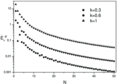
Figure 1: Radiated gravitational energy, $\dot{E}_{n}^{gr}$ in units $G\mu^{2}$. For the 2-2 kinky loop the energy radiation is drawn logarithmically as a function of the mode number $N$ in units of $G\mu^{2}$ for different values of parameter $k$.

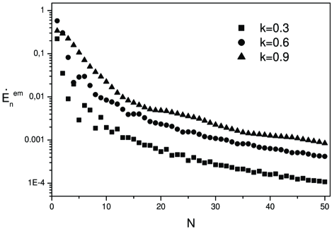
Figure 2: Radiated electromagnetic energy, $\dot{E}_{n}^{em}$ in units $q^{2}\mu$. For the 2-2 kinky loop the energy radiation is drawn logarithmically as a function of the mode number $N$ in units of $q^{2}\mu$ for different values of parameter $k$.

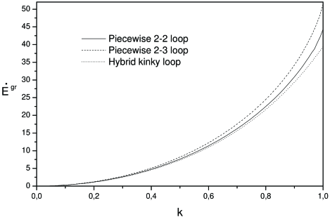
Figure 3: Total radiated gravitational energy $\dot{E}^{gr}$ in units $G\mu^{2}$ for the 2-2, 2-3 piecewise and hybrid kinky loops is shown as a function of parameter $k$. For 2-2 loop $\alpha=\pi/2$, for 2-3 loop $\beta=\pi/4$, for hybrid loop $\gamma=0$.

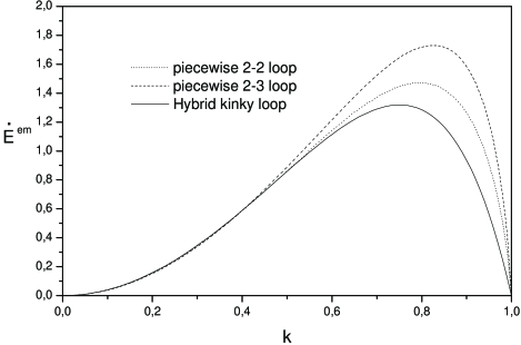
Figure 4: Total radiated electromagnetic energy $\dot{E}^{em}$ in units $q^{2}\mu$ for the 2-2, 2-3 piece-wise and hybrid kinky loop is shown as a function of parameter $k$. For 2-2 loop $\alpha=\pi/2$, for 2-3 loop $\alpha=\pi/4$, for hybrid loop $\alpha=0$.

As the first example let us consider the following chiral string loop:

$$\mathbf{a}\!=\!\mathbf{A}\!\left\{\!\begin{array}[]{lcl}\left(\xi-\pi/2\right),&&\!\!\!0\leq\xi\leq\pi,\\ \left(3\pi/2-\xi\right),&&\!\!\!\pi\leq\xi\leq 2\pi,\\ \end{array}\right.\mathbf{b}\!=\!k\mathbf{B}\!\left\{\!\begin{array}[]{lcl}\left(\eta-\pi/2\right),&&\!\!\!0\leq\eta\leq\pi,\\ \left(3\pi/2-\eta\right),&&\!\!\!\pi\leq\eta\leq 2\pi,\\ \end{array}\right.$$ (67)

where $\mathbf{A}$ and $\mathbf{B}$ are arbitrary constant unit vectors with the angle $\alpha$ between them. This is the generalization of ordinary piece-wise linear loop without the current [5] to the chiral current case. The both $a$- and $b$-loops consist of two linear segments. We call this loop as 2-2 piece-wise loop. It has such a symmetry that no momentum or angular momentum are radiated. The dependence of radiated electromagnetic and gravitational energy on the mode number $l$ is shown in Fig. 1 and 2 for the case of 2-2 piece-wise loop with $\alpha=\pi/2$. The decreasing of radiated energy with mode number $l$ is more pronounced for larger current, as it should be physically, because the maximal speed of the string is decreasing with the increasing of the current. In the case of electromagnetic radiation besides the overall decreasing of energy with the mode number one can see in Fig. 2 also the weak oscillations of energy rate. The period of this oscillation is increasing with $k$. In the Fig. 3 and 4 the dependence of total radiated energy is shown as a function of parameter $k$ for $\alpha=\pi/2$. It is seen the monotonous increasing of the gravitational energy radiation with the $k$ (i. e. with the decreasing of the string current). At the same time the electromagnetic energy radiated by the string has a maximum near $k\sim 0.9$. For $k=0$ (no current on the string) our result for gravitational radiation $\dot{E}^{\rm{gr}}_{\rm{max}}=44.36G\mu^{2}$ reproduces the result of Garfinkle and Vachaspati [5]. The corresponding graphs for other values of $\alpha$ look similar. The maximum values of energy rates $\dot{E}^{\rm{gr}}_{\rm{max}}$ and $\dot{E}^{\rm{em}}_{\rm{max}}$ increase with decreasing of $\alpha$. While $k$ at which the maximum is reached for gravitational radiation rate is $k=1$ exactly and for electromagnetic radiation rate $k\sim 0.9$ respectively.

5.2 2-3 piece-wise loop

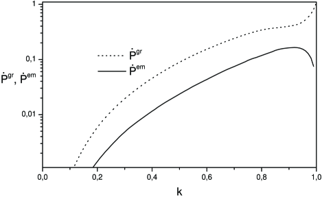
Figure 5: Total radiated electromagnetic $|\dot{P}^{em}|$ momentum in units $q^{2}\mu$ and gravitational $|\dot{P}^{gr}|$ momentum in units $G\mu^{2}$ for 2-3 kinky loop is shown as a function of parameter $k$.

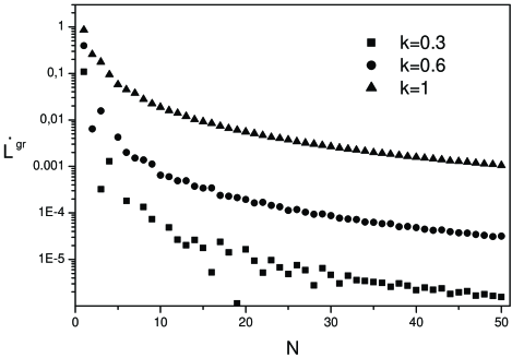
Figure 6: Radiated gravitational angular momentum $\dot{L}^{gr}$ in units $\mathcal{L}G\mu^{2}$ for the 2-3 kinky loop is shown as a function of mode number $N$ for different values of parameter $k$.

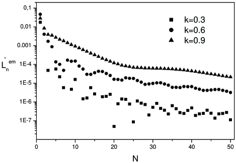
Figure 7: Radiated electromagnetic angular momentum $\dot{L}^{em}$ in units $\mathcal{L}q^{2}\mu$ for the 2-3 kinky loop is shown as a function of mode number $N$ for different values of parameter $k$.

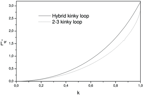
Figure 8: Total radiated gravitational angular momentum $\dot{L}^{gr}$ in units $\mathcal{L}G\mu^{2}$ for 2-3 kinky loop and hybrid loop is shown as a function of parameter $k$.

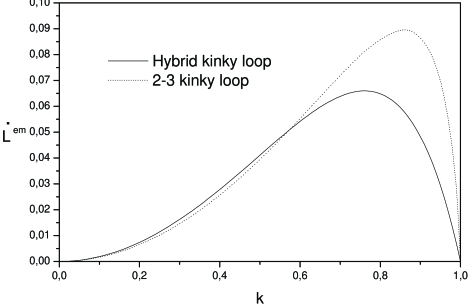
Figure 9: Total radiated electromagnetic angular momentum $\dot{L}^{em}$ in units $\mathcal{L}q^{2}\mu$ for 2-3 kinky loop and hybrid loop is shown as a function of parameter $k$.

As the second example we consider the piece-wise linear loop of the following configuration (the generalization of the loop, considered in [9]): $a$-loop consists of 2 segments and lies along the $z$- axis. One kink of $a$-loop is positioned at the origin ($\xi=0$) and the another kink ($\xi=\pi/2$) has coordinates $(0,0,\pi/2)$. The positions of kinks of $b$-loop are given by the following coordinates: the first kink at $\eta=0$ is positioned at the origin; the second kink at $\eta=\pi/3$ has coordinates $-({k\pi}/{3})(\cos\beta,\sqrt{3},\sin\beta)$ and the third kink at $\eta=2\pi/3$ has coordinates $({k\pi}/{3})(\cos\beta,-\sqrt{3},\sin\beta)$. We call this loop as 2-3 piece-wise loop. Total radiated energy rates into the gravitational and electromagnetic waves for $\beta=\pi/4$ are shown in Fig. 3 and 4. This loop radiates also momentum and angular momentum. In the Fig. 5 the total momentum rates into electromagnetic and gravitational waves are shown for $\beta=\pi/4$. The corresponding rates for angular momentum as a function of the mode number are shown in Fig. 6 and Fig. 7 for $\beta=0$. Again one can see that the angular momentum radiation rate into the electromagnetic waves weakly oscillates with mode number. The total angular momentum radiations are shown in Fig. 8 and Fig. 9. The graphs for momentum and angular momentum rates look very similar to graphs for energy radiation: in the case of gravitational radiation the increasing of corresponding rates are monotonous with $k$. While for electromagnetic radiation the radiation of momenta has maximums near $k=0.9$.

5.3 Hybrid kinky loop

As the third example let us consider the loop of the following configuration:

$$\mathbf{a}=(\sin\xi,\;-\cos\xi,\;0),\quad\mathbf{b}=k\mathbf{B}\left\{\begin{array}[]{lcl}\left(\eta-\pi/2\right),&&0\leq\eta\leq\pi,\\ \left(-\eta+3\pi/2\right),&&\pi\leq\eta\leq 2\pi.\\ \end{array}\right.$$ (68)

The $a$-loop in this example is a circle in the $(x,y)$ plane and $\mathbf{B}\!=\!(\cos\gamma;0;\sin\gamma)$. For $\gamma=\pi/2$ the gravitational and electromagnetic radiated energy and angular momentum are shown on the Fig. 3, 4, 8 and 9. The total gravitational energy radiation for $k=1$ coincides with the result of Allen et. al [8] ($\dot{E}^{\rm{gr}}\simeq 39.0G\mu^{2}$). For $\gamma=\pi/4$ the results are presented in the Table 1.

Table 1: The radiation rates from hybrid kinky loop

k	0.00	0.25	0.50	0.75	1.00
$\dot{E}^{\rm gr}$	0.00	1.79	7.56	19.10	46.58
$\dot{E}^{\rm em}$	0.00	0.23	0.86	1.60	0.00
$\dot{L}^{\rm gr}$	0.00	0.19	0.81	1.11	6.20
$\dot{L}^{\rm em}$	0.00	0.008	0.029	0.059	0.0

Table 2: The cosine of deviation angle between $\dot{\mathbf{L}}^{\rm{gr}}$ and $\dot{\mathbf{L}}^{\rm{em}}$ and $\mathbf{L}_{st}$

	k	0.25	0.5	0.75	1
2-3 loop,	$\varepsilon^{gr}$	-0.94	-0.94	-0.95	-0.96
$\beta=\pi/4$	$\varepsilon^{em}$	-0.98	-0.98	-0.99	-
hybrid loop,	$\varepsilon^{gr}$	-0.97	-0.97	-0.97	-0.97
$\gamma=\pi/4$	$\varepsilon^{em}$	-0.78	-0.88	-0.98	-

Durrer in [10] found that the radiated angular momentum for some particular class of ordinary cosmic string loops $\mathbf{\dot{L}}^{gr}$ is antiparallel to the stationary angular momentum $\mathbf{L}_{st}$ of the loop. It means that angular momentum of the loops always decreases with time due to gravitational radiation. Our results for angular momentum radiation into electromagnetic and gravitational waves for string loops with chiral current agree in general with the results of Durrer. The chiral loops considered in this paper also lose angular momentum with time. But unlike the examples considered by Durrer we found that for some configurations of chiral loops $\mathbf{\dot{L}}^{\rm gr}$ and $\mathbf{\dot{L}}^{\rm em}$ are not exactly antiparallel to total angular momentum of the loop $\mathbf{L}_{\rm st}$, but deviate on some small angle. In the Table 2 the values $\varepsilon^{\rm gr}=(\mathbf{\dot{L}}^{\rm gr}\mathbf{L}_{\rm st})/|\mathbf{\dot{L}}^{\rm gr}||\mathbf{L}_{\rm st}|$ and $\varepsilon^{\rm em}=(\mathbf{\dot{L}}^{\rm em}\mathbf{L}_{\rm st})/|\mathbf{\dot{L}}^{\rm em}||\mathbf{L}_{\rm st}|$, determining the angle between $\mathbf{\dot{L}}$ and $\mathbf{L}_{\rm st}$ are presented for 2-3 piece-wise loop with $\beta=\pi/4$ and hybrid kinky loop with $\gamma=\pi/4$. Note that for symmetric configurations $\beta=0$ and $\gamma=0$ the angular momentum radiation $\mathbf{\dot{L}}^{\rm gr}$, $\mathbf{\dot{L}}^{\rm em}$ is exactly antiparallel to $\mathbf{L}_{\rm st}$ at any $k$.

6 Conclusion

We found the general formulas for gravitational and electromagnetic energy, momentum and angular momentum radiation rates into the unit solid angle from chiral cosmic string loops. The main new result of the paper is the presentation of the radiation rates from oscillating string loops in the integral form. In the corresponding integrals the summations of infinite mode series have been performed analytically. The derived expressions for $d\dot{E}/d\Omega$, $d\dot{\mathbf{P}}/d\Omega$ and $d\dot{\mathbf{L}}/d\Omega$ contain four-dimensional integrals, which depend on the particular loop configuration. The derived integral presentation is especially convenient for numerical calculations in comparison with a weakly convergent summation over modes. To find the total rates of radiated energy, momentum and angular momentum one should integrate the obtained expressions over unit sphere. The final expressions for gravitational and electromagnetic radiation can be written in the following form:

$$\dot{E}^{\rm{gr}}=\Gamma_{E}^{\rm{gr}}G\mu^{2},\,\dot{P}^{\rm{gr}}=\Gamma_{P}^{\rm{gr}}G\mu^{2},\,\dot{L}^{\rm{gr}}=\Gamma_{L}^{\rm{gr}}\mathcal{L}G\mu^{2},$$

$$\dot{E}^{\rm{em}}=\Gamma_{E}^{\rm{em}}\mu q^{2},\dot{P}^{\rm{em}}=\Gamma_{P}^{\rm{em}}\mu q^{2},\dot{L}^{\rm{em}}=\Gamma_{L}^{\rm{em}}\mathcal{L}\mu q^{2},$$ (69)

where numerical coefficients $\Gamma$ depend on the loop configuration (and also on the current along the loop). Applying our formulas to some examples of chiral string loop configurations we calculated numerically coefficients $\Gamma$ as functions of $k$.

In this paper the following three family of examples have been considered: (i) the piece-wise linear kinky loop with $a$ and $b$-loop consisting of two straight parts (2-2 piece-wise loop); (ii) the piece-wise linear loop such that $a$-loop consists of two segments and $b$-loop consists of three segments (2-3 piece-wise loop); (iii) the hybrid loop in which $a$-loop is circle and $b$-loop consists of two straight parts (hybrid kinky loop). For first and second examples the four-dimensional integrals in our expressions for radiated energy, momentum and angular momentum become the multiple sums over the kinks. These sums can be analytically calculated using the symbolic computation on computer (e. g. “Mathematica” packet). To obtain the radiation for third example (hybrid loop) we calculated two-dimensional integrals (originated from the smooth $a$-loop) and summed over the kinks of $b$-loop. Unfortunately, we could not carry out the calculations for strings with $a$ and $b$ loops being arbitrary smooth closed curves because the corresponding calculations of four-dimensional integrals take an enormous amount of time.

For considered examples we observe weak oscillations of the electromagnetic radiation as a function of mode number. These oscillations (accompanied with a general decreasing of the radiation rate with mode number) have the different periods depending on the current along the string: the larger current the smaller the period of oscillations. This effect does not take place for gravitational radiation.

The total gravitational radiation of energy, momentum and angular momentum behave in a similar way. They increase slowly with $k$, when $k$ is small (and the current is large) and rapidly increase at large $k$ (or at large current). In total the gravitational radiation rates are increasing monotonous functions of $k$. For the electromagnetic radiation the situation is different: the losses of energy, momentum and angular momentum into electromagnetic waves for all considered examples have maximum near $k\sim 0.9$, i. e. when the current is rather small. For considered examples the maximal coefficients in (6) have the following values:

$$\Gamma_{E}^{\rm{gr}} \simeq 50,\quad\Gamma_{P}^{\rm{gr}}\simeq 1,\quad\Gamma_{L}^{\rm{gr}}\simeq 3,$$

$$\Gamma_{E}^{\rm{em}} \simeq 2,\quad\Gamma_{P}^{\rm{em}}\simeq 0.1,\quad\Gamma_{L}^{\rm{em}}\simeq 0.1.$$ (70)

We also have found, that for some non-symmetric examples of chiral loops, the radiated angular momentum $\dot{\mathbf{L}}$ into electromagnetic and gravitational waves is not exactly opposite to the angular momentum of the loop $\mathbf{L}_{st}$, but slightly differ from it (even when there is no current on the string), unlike the other types of loops considered by Durrer [10].

References

- [1] E. P. S. Shellard and A. Vilenkin, Cosmic Strings and other Topological Defects (Cambridge University Press, Cambridge, England, 1994).
- [2] M. B. Hindmarsh and T. W. B. Kibble, Rep. Prog. Phys. 58, 477 (1995).
- [3] T. Vachaspati and A. Vilenkin, Phys. Rev. 31, 3052 (1985).
- [4] C. Burden, Phys. Lett. 164B, 277 (1985).
- [5] D. Garfinkle and T. Vachaspati, Phys. Rev. D 36, 2229 (1987).
- [6] T.Damour and A. Vilenkin, Phys. Rev. Lett. 85, 3761 (2000).
- [7] B.Allen and P.Casper, Phys.Rev. D50, 2496 (1994).
- [8] B.Allen, P.Casper and A. Ottewill, Phys. Rev. D50, 3703 (1994).
- [9] B.Allen, P.Casper and A. Ottewill, Phys. Rev. D51, 1546 (1995).
- [10] R. Durrer, Nucl. Phys. B328, 238 (1989).
- [11] E. Witten, Nucl. Phys. B249, 557 (1985).
- [12] B. Carter and P. Peter, Phys. Lett. B466, 41 (1999).
- [13] A. C. Davis, T. W. B. Kibble, M. Pickles and D.A. Steer, Phys. Rev. D 62 (2000) 083516.
- [14] J.J. Blanco-Pillado, Ken D. Olum and A. Vilenkin, Phys. Rev. D 63, 103513.
- [15] J.J. Blanco-Pillado and Ken D. Olum, Nucl. Phys. B599 (2001) 435.
- [16] E.Babichev and V.Dokuchaev, Phys. Rev. D 66, 025007 (2002).
- [17] S. Weinberg, Gravitation and Cosmology (Wiley, New York, 1974).
- [18] I.S. Gradshteyn and I.M. Ryzhik, Tables of Integrals, Series and Products (Academic, New York, 1980).
- [19] L.D. Landau and E.M. Lifshitz, The Classical Theory of Fields (Pergamon, New York, 1975), 4th ed.
- [20] A. Vilenkin and T. Vachaspati, Phys.Rev.Lett 58, 1041 (1987).