Hubble Space Telescope Evidence for an Intermediate-Mass Black Hole in the Globular Cluster M15—
I. STIS Spectroscopy and WFPC2 Photometry

Abstract

In this series of two papers we describe a project with the Space Telescope Imaging Spectrograph (STIS) on Hubble Space Telescope (HST) to measure the line-of-sight velocities of stars in the central few arcsec of the dense globular cluster M15. The main goal of this project is to search for the possible presence of an intermediate mass central black hole. This first paper focuses on the observations and reduction of the data. We ‘scanned’ the central region of M15 spectroscopically by consecutively placing the $0.1^{\prime\prime}$ HST/STIS slit at 18 adjacent positions. The spectral pixel size exceeds the velocity dispersion of M15. This puts the project at the limit of what is feasible with STIS, and exceedingly careful and complicated data reduction and analysis were required. We applied corrections for the following effects: (a) drifts in the STIS wavelength scale during an HST orbit; (b) the orbital velocity component of HST along the line-of-sight to the cluster, and its variations during the HST orbit; and (c) the apparent wavelength shift that is perceived for a star that is not centered in the slit. The latter correction is particularly complicated and requires many pieces of information: (1) the positions and magnitudes of all the stars near the center of M15; (2) the accurate positionings of the STIS slits during the observations; (3) and the HST/STIS point-spread function (PSF) and line-spread function (LSF). To address the first issue we created a stellar catalog of M15 from the existing HST/WFPC2 data discussed previously by Guhathakurta et al. (1996), but with an improved astrometric and photometric calibration. The catalog is distributed electronically as part of this paper. It contains 31,983 stars with their positions and U, B and V magnitudes. To address the second issue we model the observed intensity profiles along the STIS slits to determine the slit positionings to $0.007^{\prime\prime}$ accuracy in each coordinate. To address the third issue we obtained observations of a bright field star to which we fitted multi-Gaussian PSF and LSF models. Upon reduction of the M15 spectroscopy we ultimately obtain 19,200 one-dimensional STIS spectra, each for a different aperture position in M15, with a velocity scale accurate to better than $2.5\>{\rm km}\,{\rm s}^{-1}$. We develop an algorithm that co-adds the spectra for individual apertures and use it to extract spectra of individual stars with minimum blending and maximum $S/N$. In Paper II (Gerssen et al.) we use these spectra to extract reliable line-of-sight velocities for 64 stars, half of which reside within $R=2.4^{\prime\prime}$ from the cluster center. These velocities constrain the central structure, dynamics and mass distribution of the cluster.

1 Introduction

This is the first in a series of two papers in which we present the results of a study with the Hubble Space Telescope (HST) of the line-of-sight velocities of stars in the central few arcsec of the globular cluster M15 (NGC 7078). The present paper discusses the spectroscopic observations with the HST Space Telescope Imaging Spectrograph (STIS) and the extraction and calibration of the stellar spectra. It also discusses the construction of a photometric catalog from HST imaging with the Second Wide Field and Planetary Camera (WFPC2), which proved essential in the reduction and interpretation of the data. The second paper (Gerssen et al. 2002, hereafter Paper II) discusses the determination of line-of-sight velocities from the spectra, and the implications for the dynamics and structure of M15. The main motivation for our study is to better constrain the possible presence of an intermediate-mass black hole in the center of M15. Such a black hole was hinted at by previous work (e.g., Peterson, Seitzer & Cudworth 1989; Gebhardt et al. 2000a), but the limited quality of the data precluded very strong conclusions (see the review in van der Marel 2001).

The globular cluster M15 at a distance of 10 kpc has one of the highest central densities of any globular cluster in our Galaxy. The high density has likely affected the stellar population, as evidenced by the presence of two bright X-ray sources (White & Angelini 2001) and several millisecond pulsars (Phinney 1993). A variety of interesting dynamical and structural evolutionary phenomena have been predicted to occur at high stellar densities, including mass segregation and the possible formation of a central black hole (Hut et al. 1992; Meylan & Heggie 1997; see the additional discussion in the introductory section of Paper II). As a result, M15 has been one of the globular clusters for which the structure and dynamics have been most intensively studied in the past decade.

Studies of the dynamics of M15 have focused primarily on the determination of line-of-sight velocities of individual stars, using either spectroscopy with single apertures, long-slits or fibers (Peterson et al. 1989; Dubath & Meylan 1994; Dull et al. 1997; Drukier et al. 1998), or using imaging Fabry-Perot spectrophotometry (Gebhardt et al. 1994, 1997, 2000a). Integrated light measurements using single apertures have also been attempted (Peterson et al. 1989; Dubath, Meylan & Mayor 1994), but are only of limited use; integrated light spectra are dominated by the light from only a few bright giants, and as a result, inferred velocity dispersions are dominated by shot noise (Zaggia et al. 1992, 1993; Dubath et al. 1994).

Line-of-sight velocities are now known for $\sim\!1800$ M15 stars, as compiled and analyzed by Gebhardt et al. (2000a). The projected velocity dispersion profile increases inwards from $\sigma=3\pm 1\>{\rm km}\,{\rm s}^{-1}$ at $R=7$ arcmin, to $\sigma=11\pm 1\>{\rm km}\,{\rm s}^{-1}$ $R=24^{\prime\prime}$. The velocity dispersion is approximately constant at smaller radii, and is $\sigma=11.7\pm 2.8\>{\rm km}\,{\rm s}^{-1}$ at the innermost available radius $R\approx 1^{\prime\prime}$. The rotational properties of M15 are quite peculiar. The position angle of the projected rotation axis in the central region is $\sim\!100^{\circ}$ different from that at larger radii, and the rotation amplitude increases to $V_{\rm rot}=10.4\pm 2.7\>{\rm km}\,{\rm s}^{-1}$ for $R\lesssim 3.4^{\prime\prime}$, so that $V_{\rm rot}/\sigma\approx 1$ in this region. A plausible explanation for these properties is still lacking.

To improve our understanding of the central mass distribution in M15, it is of crucial importance to obtain more stellar velocities close to the center. However, velocity determinations at $R\lesssim 2^{\prime\prime}$ are very difficult due to severe crowding and the presence of a few bright giants in the central arcsec. Gebhardt et al. (2000a) used an Imaging Fabry-Perot spectrophotometer with adaptive optics on the CFHT, and obtained FWHM values as small as $0.09^{\prime\prime}$. However, the Strehl ratio was only $\lesssim 6$%, so that even in these observations the light from the fainter turnoff and main-sequence stars in the central arcsec was overwhelmed by the PSF wings of the nearby giants. As a result, there are only 5 stars with known velocities within $R\leq 1.3^{\prime\prime}$ from the cluster center. To improve upon this situation we initiated the project on which we report here, in which we used HST/STIS to map the center of M15 spectroscopically at high spatial resolution. In the future, additional kinematic data on M15 may come available from stellar proper motion measurements with HST, using techniques such as those described by Anderson & King (2000). However, at present no such measurements are available.

This paper is organized as follows. Section 2 describes the construction of a stellar catalog from WFPC2 data. This catalog is essential for a proper interpretation of the M15 spectra. It is distributed electronically as part of the present paper. Section 3 describes STIS spectra of a bright field star which were obtained to calibrate the STIS point spread function (PSF) and line-spread function (LSF). Section 4 describes the M15 STIS spectroscopy, the observational setup and data reduction, and an analysis of the achieved slit positioning accuracies. The velocity calibration accuracy of the spectra is the most crucial aspect of the observations, and this issue is discussed in detail. Section 5 discusses the algorithm adopted for the extraction of individual stellar spectra. These spectra form the end-product of the present paper. They are used in Paper II to determine line-of-sight velocities and to study the structure and dynamics of M15. Section 6 presents concluding remarks.

2 Construction of a Stellar Catalog

For proper planning and interpretation of long-slit spectra of M15 it is necessary to know the positions and magnitudes of the stars in M15. Because M15 is dense, and its central regions are crowded, it is important to determine these quantities from high spatial resolution data. Several imaging studies of M15 were undertaken with the HST in the years 1990-1994 (Lauer et al. 1991; Ferraro & Paresce 1993; Stetson 1994; de Marchi & Paresce 1994; Yanny et al. 1994), but these suffered from the aberrated HST PSF. Imaging studies with the Faint Object Camera (FOC) on the refurbished HST (with COSTAR) were reported by de Marchi & Paresce (1996) and Sosin & King (1997). However, while FOC provided a sharp and well-sampled PSF, it had only a very small field of view and its data were hard to calibrate accurately. Data from WFPC2 are therefore preferable; see Biretta et al. (2001) for a detailed description of this instrument.

2.1 WFPC2 observations

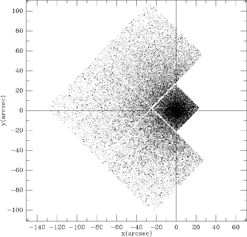
Figure 1: Spatial distribution of the stars in the stellar catalog of M15. North is to the top and East is to the left. All the stars in the catalog are shown; brighter stars are indicated with slightly larger symbols. The footprints of the WFPC2 field of view and of the individual CCDs are clearly visible. The cluster center determined by G96 is at the origin. The cross marks the star that was used to perform target acquisitions with STIS.

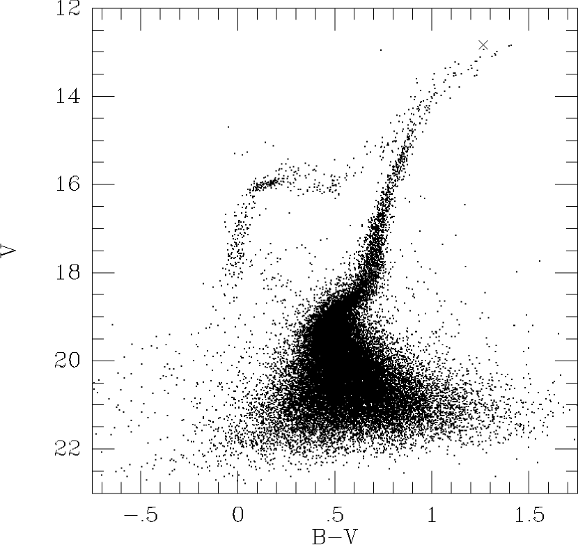
Figure 2: CMD of $V$ vs. $B-V$ for the stars in the stellar catalog of M15. The cross near the tip of the red giant branch marks the star that was used to perform target acquisitions with STIS.

WFPC2 images of M15 were obtained on April 7, 1994 in the context of HST program GO-5324 (PI: Yanny). Results from these observations were reported in a study led by one of us (Guhathakurta et al. 1996, hereafter G96). Data were obtained using the filters F336W, F439W and F555W, respectively, which correspond roughly to the Johnson U, B and V bands. The G96 paper provides a detailed discussion of the data acquisition and reduction. Their figure 1 shows a large scale black-and-white image of M15, while their figure 2 shows a ‘true-color’ image of the central $9^{\prime\prime}\times 9^{\prime\prime}$. The photometric analysis of G96 yielded a list of stars, and for each star its position on one of the WFPC2 chips and the countrate in each of the filters. This list is the starting point of the present analysis. While G96 applied both an astrometric calibration (the transformation from chip position to right ascension RA and declination DEC) and a photometric calibration (the transformation from count-rate to Johnson U, B and V magnitudes) to their star list, these were not particularly accurate. The WFPC2 had only just been installed on HST when the G96 data were obtained, and there was little information available on the appropriate astrometric and photometric transformation equations when their paper was written. This was not a problem for the G96 study, which focused on a determination of the stellar number density profile of M15. However, for the present application both astrometric and photometric accuracy are important, and we therefore decided to apply an improved calibration to the G96 star list.

2.2 Astrometric Calibration

For the astrometric calibration we first ran the IRAF/STSDAS task uchcoord, as recommended by the HST Data Handbook (Voit et al. 1997). This properly sets the image header parameters for the WFPC2 plate scales and chip-to-chip rotations. The task metric was then used to transform the pixel coordinates of each star to RA and DEC in the Guide Star Coordinate System (GSCS). For the position of the M15 cluster center we adopted the pixel position calculated by G96 (which has an estimated $1\sigma$ uncertainty of $0.2^{\prime\prime}$ in each coordinate). For each star the relative position with respect to the cluster center is given by $\Delta{\rm RA}={\rm RA}-{\rm RA}_{\rm cen}$ and $\Delta{\rm DEC}={\rm DEC}-{\rm DEC}_{\rm cen}$. In the following it is more convenient to work in a right-handed Cartesian coordinate system, so we define $x=-\Delta{\rm RA}$ and $y=\Delta{\rm DEC}$. The 1$\sigma$ absolute accuracy of the GSCS is only $\sim 0.5^{\prime\prime}$. However, the absolute astrometric accuracy can be improved using the star AC211. This X-ray source has a radio counterpart for which the position is determined to within $0.1^{\prime\prime}$ accuracy. Kulkarni et al. (1990) find for AC211 that ${\rm RA}=21{\rm h}\>29{\rm m}\>58.310{\rm s}$ and ${\rm DEC}=12^{\circ}\>10^{\prime}\>02.85^{\prime\prime}$. We find for AC211 that $x=0.37^{\prime\prime}$ and $y=1.96^{\prime\prime}$. This implies that the M15 cluster center is at ${\rm RA}=21{\rm h}\>29{\rm m}\>58.335{\rm s}$ and ${\rm DEC}=12^{\circ}\>10^{\prime}\>00.89^{\prime\prime}$ in the radio coordinate system. This differs by $0.55^{\prime\prime}$ from the position that was calculated in GSCS, consistent with the absolute accuracy of the latter.

2.3 Photometric Calibration

For the photometric calibration we started with the count rates (i.e., the integrated counts divided by the exposure time) determined by G96. These had been corrected to an equivalent aperture with a radius of $0.5^{\prime\prime}$, although the actual photometry was performed with a smaller aperture. These count rates were first corrected for geometric distortion and then for the WFPC2 Charge Transfer Efficiency (CTE) problem, as described in the HST Data Handbook (Voit et al. 1997). For the CTE correction we used the formulae given by Whitmore & Heyer (1997). However, we increased their recommended corrections by a factor 3, to take into account that the CTE was more of a problem before April 24, 1994 (i.e., when the M15 data were taken). On this date the WFPC2 temperature was lowered from $-76^{\circ}$C to $-88^{\circ}$C. The factor of 3 was chosen on the basis of quantitative comparisons of the CTE effect at the two different temperatures (Holtzman et al. 1995a). We then transformed the count rates to Johnson U, B and V magnitudes using the procedures described by Holtzman et al. (1995b). Several iterations were performed to get the color terms correct in the transformation equations. The filter- and chip-dependent change in throughput that occurred on April 24, 1994 was taken into account, using the values given in the WFPC2 Data Handbook (Voit et al. 1997).

The above steps provide an optimal relative photometric calibration for the data. However, the absolute calibration remains uncertain due to uncertainties in aperture corrections and contamination-related throughput corrections. This is the case for WFPC2 data in general, but is particularly important for data taken before April 24, 1994. WFPC2 was operated at $-76^{\circ}$C for only a few months, and the instrument calibrations available for this period are considerably less accurate than those available for subsequent data. We therefore applied a constant additive correction to all the stellar magnitudes for a given filter+CCD combination. The corrections were chosen to align the red giant branch (RGB) and horizontal branch (HB) features in color-magnitude diagrams (CMDs) with the corresponding features in well-calibrated ground-based data (Durrell & Harris 1993; Stetson 1994). The corrections ranged from $0.1$–$0.3$ mag. With these corrections we estimate the calibration of the final catalog to be accurate to $\sim 0.03$ mag in $B$ and $V$ and to $\sim 0.05$ mag in $U$. This is sufficient for the purposes of the present project.

2.4 Properties of the Stellar Catalog

The final stellar catalog contains 31,983 stars with their positions and U, B and V magnitudes. It is distributed electronically as part of this paper. For reference, the first 25 entries are listed in Table 1. Each star has an ID number. These numbers were already used for cross-identification purposes by Gebhardt et al. (2000a) in their compilation of M15 stars with ground-based line-of-sight velocity determinations. The spatial distribution of the stars in our WFPC2 catalog is shown in Figure 1. The footprint of the WFPC2 field of view is clearly visible. Towards the East the catalog extends as far as $2.0$ arcmin from the cluster center. For comparison, the half-mass radius of M15 is $1.06$ arcmin and the tidal radius is $22.1$ arcmin (Harris 1996), so the catalog only covers the central part of M15. Note from Figure 1 that stars are not detected along the CCD chip boundaries. Stars within $14.9^{\prime\prime}$ from the cluster center are all detected on the PC chip, and this inner region of M15 is therefore spatially complete in the catalog.

Figure 2 shows a CMD of $V$ vs. $B-V$ for the stars in the catalog. The well-known stellar-evolutionary features of the main sequence, subgiant branch, RGB, HB, and blue stragglers are all easily discernible. The increased width of the HB between $0.2\lesssim B-V\lesssim 0.5$ (the instability strip) is due to RR Lyrae variables. The implications of the morphology and position of the observed CMD features for the age, metallicity and stellar population of M15 have all been addressed previously (e.g., Durrell & Harris 1993; Ferraro & Paresce 1993; Stetson 1994; de Marchi & Paresce 1994; Yanny et al. 1994; de Marchi & Paresce 1996; Sosin & King 1997) and will not be discussed here. The large color spread of the main sequence at faint magnitudes is due to photometric errors. The photometric errors and completeness of the catalog, and their dependence on distance from the cluster center, were discussed in detail by G96. The catalog is essentially complete for magnitudes brighter than $V\approx 19$, and the completeness drops steadily towards fainter magnitudes. No stars are detected fainter than $V\approx 22.5$.

3 STIS Calibration Spectroscopy of a Field Star

We were awarded 25 orbits in the context of HST program GO-8262 (PI: van der Marel) for a spectroscopic study of the central region of M15. All observations were taken with STIS (see Leitherer et al. 2001 for a detailed description of this instrument). For all observations we used the 52X0.1 slit, which has a calibrated width of $0.095^{\prime\prime}$ (Bohlin & Hartig 1998). As dispersive element we used the G430M grating centered at a wavelength of 5216Å. This yields spectra that cover the region from 5073—5359Å. This wavelength range has often been used for kinematical studies and it includes the Mg b triplet region around 5175Å. The pixel size in the spatial direction is $0.05071^{\prime\prime}$ (Bowers & Baum 1998). The pixel size in the spectral direction is 0.276Å. The latter corresponds to $15.86\>{\rm km}\,{\rm s}^{-1}$ at the center of the wavelength range. For comparison, the central velocity dispersion of M15 has previously been measured to be $\sigma\approx 12\>{\rm km}\,{\rm s}^{-1}$ (Gebhardt et al. 2000a), so for a proper understanding of the M15 kinematics the Doppler shifts must be measured to a fraction of a pixel accuracy. This requires accurate calibration, and a detailed understanding of the STIS point spread function (PSF) and line-spread function (LSF). For this reason we used one orbit on June 14, 1999, for a set of calibration observations of a bright field star.

3.1 Observations

For the calibration observations we chose to observe the star HD 122563, an extremely metal-poor field giant with magnitude $V=6.2$. At the start of the orbit an ACQ acquisition procedure was executed to put the star near the center of the slit. This procedure has a nominal accuracy between $0.01^{\prime\prime}$ (Leitherer et al. 2001) and $0.025^{\prime\prime}$ (Voit et al. 1997). It was not necessary to achieve better pointing accuracy than this, so we did not perform an additional (more accurate) ACQ/PEAK procedure. A series of small telescope slews were then used to successively position the star at 14 different positions relative to the slit, as shown schematically in Figure 3. At each position two spectra were obtained. These were dithered by an integer number of $\pm 2$ pixels in the direction parallel to the slit, to allow removal of CCD defects during data reduction. The exposure times ranged from 2 to 20 seconds per exposure. The longer exposure times were used when the star was offset perpendicularly from the center of the slit, so as to obtain an approximately similar signal-to-noise ratio ($S/N$) for all exposures. We used 2-pixel on-chip binning in the spatial direction to obtain an effective pixel size of $0.1014^{\prime\prime}$.

The STIS Mode Selection Mechanism (which selects and positions the grating) has a small mechanical non-repeatability. This causes an uncertainty (amounting to a few pixels) in the relative position of the 2D spectrum with respect to the CCD rows and columns. In addition, slight drifts in this position (of the order of $0.1$ pixel) can occur over the course of an orbit. For accurate calibration it is therefore important that contemporaneous spectra of an arc lamp are obtained. For the calibration star observations we obtained five exposures of an arc lamp, spread equally in time between the beginning and the end of the orbit.

3.2 Data Reduction

Our data reduction procedures are based on the default STIS reduction pipeline. However, we applied a number of modifications and additional calibrations to obtain more accurate results. We started with the raw data files, and used the IRAF/STSDAS task getref to ensure that the relevant header keywords point to the most appropriate calibration files. Subsequently, the basic2d task was run to perform the tasks of data quality initialization, bias subtraction, dark current subtraction, and flat-fielding. For the dark current subtraction we used the ‘superdark’ frames that are generated by STScI on a weekly basis. We experimented with the use of daily darks, but found that they did not improve the results due to their lower $S/N$. We fitted and subtracted a spatially linear background from all frames to ensure that source-free regions along the slit were consistent with zero. The two exposures obtained at each stellar position were then aligned and co-added. The latter was done with the task ocrrej, which rejects cosmic rays and CCD defects. Bad columns were corrected using linear interpolation. After these steps a significant number of bad pixels remain in the data. Positive outliers are generally pixels that are ‘hot’ in the data frame but normal in the (non-contemporaneous) dark frame, while for negative outliers the opposite is generally the case. All outliers were interpolated over using the task cosmicrays (to find the negative outliers the science frame was multiplied by minus one).

The arc lamp spectra were reduced similarly as the object spectra. The wavecal task was then used to determine the shift of the spectra with respect to a fiducial spectrum maintained in the HST Data Archive. These Mode Selection Mechanism (MSM) shifts were interpolated linearly in time over the course of the observations to determine the MSM shift appropriate for each individual exposure of the target.

An additional complication in the velocity calibration arises from the fact that HST moves around the Earth with an orbital velocity of $7.5\>{\rm km}\,{\rm s}^{-1}$. This can cause velocity shifts between observations taken at different times of up to $15\>{\rm km}\,{\rm s}^{-1}$. This exceeds the velocity dispersion of M15, and it is therefore imperative to correct for this. This is not normally done by the STIS/CCD pipeline. However, the support files that are created and delivered with HST data contain header keywords (VELOCSTX,VELOCSTY,VELOCSTZ) that contain the three-dimensional velocity vector of HST (as measured halfway through the exposure time). Phil Hodge (priv. comm.) kindly provided a routine to calculate the velocity component in the direction of the target, given its RA and DEC. We used this routine to calculate this velocity for each exposure.

For each exposure, the HST velocity shift was combined with the MSM wavelength shift calculated previously (using the fact that 1 pixel is $15.86\>{\rm km}\,{\rm s}^{-1}$ at the center of the wavelength range). The shifts calculated for different exposures at the same target position were then averaged, weighted by the individual exposure times. These shifts were then written to the header keywords in the co-added and reduced target spectra. The task x2d was then used to read these keywords, and perform a two-dimensional rectification to a linear heliocentric wavelength scale along rows, and a linear spatial scale along columns. This also performs a flux calibration to units of ${\rm erg}\>{\rm cm}^{-2}\>{\rm s}^{-1}\>{\rm\AA}^{-1}$.

3.3 The Influence of Spatial Undersampling

One problem in all STIS spectroscopy of point sources is the fact that the spatial pixel size of $0.05071^{\prime\prime}$ undersamples the HST PSF. For the calibration star observations we used 2-pixel on-chip binning in the spatial direction to obtain an effective pixel size of $0.1014^{\prime\prime}$, which further increases the undersampling. It is useful to have an understanding of the influence of this on the inferred spectra.

For any spectrograph, a spectrum that falls on the CCD is generally slightly titled (by of order a few degrees) with respect to the detector rows. For a point source that is well sampled, the 2D spectrum will have the appearance of a smooth tilted line. However, for a point source that is undersampled, the 2D spectrum will a have the appearance of a stairwell. During data reduction, the spectrum is interpolated and rotated to make it align with the rows of the frame. However, this does not remove any undersampling. In an undersampled situation, the rectified spectrum will on average be horizontal, but it will have the zig-zag appearance of an un-tilted stairwell. If all the rows in the rectified spectrum are summed, one recovers the correct spectral shape. However, any horizontal cut along an individual row will have strong low-frequency undulations multiplied into the spectrum.

These effects are illustrated in Figure 4, which shows the results for one of the two-dimensional spectra of the calibration star. The top curve is the rectified spectrum summed along all rows, which provides a fairly accurate representation of the actual spectrum of the star. By contrast, the bottom curve shows the spectrum for the brightest row in the rectified image. It has low-frequency undulations multiplied into the spectrum. Individual rows in all of the rectified spectra obtained for our program look similar to this. We obtained most of the M15 data without spatial rebinning, but this does not remove the undulations. It merely decreases their amplitude and increases their frequency by a factor of 2.

At first glance, one might think that an undulating spectrum such as in Figure 4 is completely useless, unless one can somehow correct for the undersampling. However, it turns out that for the present purposes these undulations are not a problem at all. We wish to measure radial velocities from the Doppler shifts in absorption lines. The absorption lines are much narrower than the undulations in the spectrum, and their positions are not in any way affected. In cross-correlation techniques one always filters out low frequency components, and we have found that this efficiently removes any influence of the undulations on the inferred velocities. Figure 5 illustrates this by showing the cross-correlation function of the two spectra shown in Figure 4, both without and with low-frequency filtering. The tests described below and in Paper II have convinced us that the undulations do not in any way compromise our ability to infer radial velocities.

3.4 Analysis

After the reduction of the calibration star data, we have 14 different two-dimensional spectra. In each spectrum there is signal in more than one row, because the STIS PSF is not a delta function. All rows that contain signal can be analyzed as separate spectra. For the analysis it proved useful to also have a single grand-total one-dimensional spectrum for each position of the calibration star. Such spectra were obtained by co-adding all rows in a given two-dimensional frame.

We wish to use the spectra to calibrate the STIS PSF and LSF. For each spectrum (either for a given row, or grand-total) we therefore extracted two numbers: (a) the total count rate per second ${\cal C}$ summed over all wavelengths; and (b) the wavelength shift ${\cal S}$ of the spectrum with respect to some fixed standard spectrum. The standard was chosen to be the grand-total spectrum obtained with the star at the origin of the coordinate system shown in Figure 3. The wavelength shifts were determined by cross-correlation, using techniques that are described in detail in Paper II.

Figure 6 shows ${\cal C}$ and ${\cal S}$ as function of the offset $X$ of the star perpendicular to the slit (defined as in Figure 3). The count-rate ${\cal C}$ was normalized arbitrarily; its absolute value scales linearly with the brightness of the star, and is of no interest in the present context. The count-rate is large if the star is centered in the slit, and of course, it drops if the star is moved further from the slit. However, the count-rate remains positive even if the star is outside the slit, due to the wings of the PSF. The peak of ${\cal C}$ identifies the center of the slit, $X_{\rm slit}$. This peak does not occur at $X=0$, which implies that the star was not perfectly centered in the slit after the target acquisition procedure.

The shift ${\cal S}$ is measured in pixels (in the wavelength direction). It is not a constant number, but shows a well-defined behavior as function of $X$. The observed behavior is easily understood qualitatively. At each wavelength, the grating makes an image of the slit on the detector. If the light that enters through the slit is not centered in the slit, then the observer perceives a shift in wavelength. Let ${\cal S}_{\rm slit}$ be the shift (with respect to the arbitrary standard) for a source placed in the center of the slit ($X=X_{\rm slit}$). If the calibration star is positioned at $X>X_{\rm slit}$, then the intensity-weighted average $X$ coordinate of the light that enters through the slit has $\langle X\rangle>X_{\rm slit}$. This is perceived as a positive wavelength shift, ${\cal S}-{\cal S}_{\rm slit}>0$. Alternatively, if $\langle X\rangle<X_{\rm slit}$, then ${\cal S}-{\cal S}_{\rm slit}<0$. If a star is moved out of the center of the slit, then initially $|{\cal S}-{\cal S}_{\rm slit}|$ increases monotonically. However, this behavior ultimately reverses. For large values of $|X-X_{\rm slit}|$ only light in the wings of the PSF enters through the slit. These wings have relatively small intensity gradients, and the slit will be illuminated more or less homogeneously. This causes $|{\cal S}-{\cal S}_{\rm slit}|$ to revert to values near zero.

It is easy to see that $|\langle X\rangle-X_{\rm slit}|$ can never be more than half the slit width, i.e., $0.0475^{\prime\prime}$ (this limit corresponds to a delta function PSF). Taking into account the anamorphic magnification of the grating, one detector pixel in the wavelength direction corresponds to $0.05733^{\prime\prime}$ (Bowers & Baum 1998). Thus one always has $|{\cal S}-{\cal S}_{\rm slit}|\leq 0.83$ pixels, or alternatively that the peak-to-peak variation in ${\cal S}$ must be less than $1.66$ pixels. The observed peak-to-peak variation in ${\cal S}$ is less, but still amounts to $0.84$ pixels (cf. Figure 6). This corresponds to $13.3\>{\rm km}\,{\rm s}^{-1}$, which is more than the M15 velocity dispersion. It is therefore important to be able to model this effect, and to correct for it in the analysis of the M15 data.

3.5 PSF and LSF Model Fitting

To model the calibration star data we consider the case of observations of a point source through a rectangular aperture. The aperture size is $A_{x}\times A_{y}$, where $A_{x}$ is the slit width and $A_{y}$ the pixel size. We adopt a coordinate system with the origin at the center of the aperture. We assume that the PSF can be modeled as a circularly symmetric sum of Gaussians,

$${\rm PSF}(r)=\sum_{i=1}^{N}\>{{\gamma_{i}}\over{2\pi\sigma_{i}^{2}}}\>\exp\left[-{\textstyle{1\over 2}}({\textstyle{r\over\sigma_{i}}})^{2}\right].$$ (1)

The individual $\gamma_{i}$ may be either positive or negative, but must satisfy $\sum_{i=1}^{N}{\gamma_{i}}=1$. The associated encircled flux curve $E(r)$ is given by

$$E(r)\>\equiv\>\int_{0}^{r}{\rm PSF}(r^{\prime})\>2\pi r^{\prime}\>dr^{\prime}\>=\>1-\sum_{i=1}^{N}{\gamma_{i}}\>\exp\left[-{\textstyle{1\over 2}}({\textstyle{r\over\sigma_{i}}})^{2}\right].$$ (2)

We assume that the aperture is perfectly rectangular, with no diffraction off the aperture edges. Let the target be a point source positioned at $(x_{0},y_{0})$. The fraction of the light from the point source that is observed through the aperture is then

$$f_{\rm tot}=\sum_{i=1}^{N}\>{{\gamma_{i}}\over 4}\>\left\{\mathop{\rm erf}\nolimits\left[{\textstyle{x_{0}+(A_{x}/2)\over\sqrt{2}\>\sigma_{i}}}\right]-\mathop{\rm erf}\nolimits\left[{\textstyle{x_{0}-(A_{x}/2)\over\sqrt{2}\>\sigma_{i}}}\right]\right\}\>\left\{\mathop{\rm erf}\nolimits\left[{\textstyle{y_{0}+(A_{y}/2)\over\sqrt{2}\>\sigma_{i}}}\right]-\mathop{\rm erf}\nolimits\left[{\textstyle{y_{0}-(A_{y}/2)\over\sqrt{2}\>\sigma_{i}}}\right]\right\},$$ (3)

where ${\rm erf}(t)$ is the error function (van der Marel 1995). The normalized intensity distribution in the $x$ direction, integrated over the $y$-direction, of the light that enters through the aperture, is

$$f(x)={1\over{f_{\rm tot}}}\times\left\{\begin{array}[]{ll}\sum_{i=1}^{N}\>{{\gamma_{i}}\over{\sqrt{8\pi}\>\sigma_{i}}}\>\exp[-{1\over 2}({{x_{0}-x}\over{\sigma_{i}}})^{2}]\>\left\{\mathop{\rm erf}\nolimits\left[{{y_{0}+(A_{y}/2)}\over{\sqrt{2}\>\sigma_{i}}}\right]-\mathop{\rm erf}\nolimits\left[{{y_{0}-(A_{y}/2)}\over{\sqrt{2}\>\sigma_{i}}}\right]\right\},&\quad|x|\leq{{A_{x}}\over 2};\\ 0,&\quad|x|>{{A_{x}}\over 2}.\end{array}\right.$$ (4)

For our observational setup, the coordinate $x$ is related to the wavelength $\lambda$ through the equation ${\rm d}x/0.05733^{\prime\prime}={\rm d}\lambda/0.276$Å. The LSF is the convolution of $f(x)$ with the additional broadening functions due to the microroughness of the grating, the natural diffraction properties of light, and the binning into pixels (van der Marel, de Zeeuw & Rix 1997). However, the latter are all to lowest order symmetric functions of wavelength that do not cause net wavelength shifts. The only net wavelength shift therefore comes from the fact that $\langle x\rangle=\int xf(x)\>{\rm d}x$ (the intensity-weighted average $x$-coordinate of the light that enters through the aperture) is generally different from zero (the x-coordinate of the aperture center). Integration of equation (4) yields

$$\langle x\rangle =x_{0}+{1\over{f_{\rm tot}}}\>\sum_{i=1}^{N}\>{{\gamma_{i}}\over{\sqrt{8\pi}\>\sigma_{i}}} \left\{\exp\left[-\left({{x_{0}+(A_{x}/2)}\over{\sqrt{2}\>\sigma_{i}}}\right)^{2}\right]-\exp\left[-\left({{x_{0}-(A_{x}/2)}\over{\sqrt{2}\>\sigma_{i}}}\right)^{2}\right]\right\}$$ (5)

$$\times\left\{\mathop{\rm erf}\nolimits\left[{{y_{0}+(A_{y}/2)}\over{\sqrt{2}\>\sigma_{i}}}\right]-\mathop{\rm erf}\nolimits\left[{{y_{0}-(A_{y}/2)}\over{\sqrt{2}\>\sigma_{i}}}\right]\right\}.$$

With the above equations we are now in a position to model the observed quantities ${\cal C}$ and ${\cal S}$. The count-rate ${\cal C}=Kf_{\rm tot}$, where $K$ is a constant that is proportional to the brightness of the target and the transmission of the telescope+instrument system. The wavelength shift ${\cal S}$ is ${\cal S}=0.276{\rm\AA}\>(\langle x\rangle/0.05733^{\prime\prime})$, or alternatively in terms of velocity, ${\cal S}=15.86\>{\rm km}\,{\rm s}^{-1}\>(\langle x\rangle/0.05733^{\prime\prime})$. The latter equation is formally valid only at the central wavelength of the grating setting, but the dependence on wavelength can be neglected in the present context.

One additional effect needs to be taken into account, namely the pixel scattering function of the CCD. A photon that falls onto a given detector pixel has a finite probability of being detected in an adjacent pixel. This effect can be quantitatively described as convolution with a kernel of size $3\times 3$ pixels. The TinyTim software package (Krist & Hook 2001) provides an approximation for this kernel at wavelengths of 4000Å and 5500Å. These can be interpolated to the central wavelength of the our observations, which yields: $(0.018,0.052,0.018\>;\>0.052,0.720,0.052\>;\>0.018,0.052,0.018)$. The convolution in the spectral direction of the CCD corresponds to a symmetric line broadening, which does affect our radial velocity measurements for M15. The only important effect in the present context is the spatial broadening along the slit. This is described by the 3 pixel convolution kernel $(0.088,0.824,0.088)$, which is the spatial projection of the $3\times 3$ kernel listed above. To obtain predictions for the observed values ${\cal C}$ and ${\cal S}$ at a pixel $i$ along the slit, one must first calculate the predictions at pixels $i-1$, $i$, and $i+1$, and then apply the convolution kernel:

$${\cal C}_{i,{\rm obs}} =0.088\>{\cal C}_{i-1}+0.824\>{\cal C}_{i}+0.088\>{\cal C}_{i+1};$$ (6)

$${\cal C}_{i,{\rm obs}}{\cal S}_{i,{\rm obs}} =0.088\>{\cal C}_{i-1}{\cal S}_{i-1}+0.824\>{\cal C}_{i}{\cal S}_{i}+0.088\>{\cal C}_{i+1}{\cal S}_{i+1}.$$ (7)

To interpret the calibration star data we need to fit several unknowns. The most important parameters to be determined are the parameters $\gamma_{i}$ and $\sigma_{i}$ that describe the multi-Gaussian PSF in equation (1). In addition, there are: (a) the constant $K$ defined through the equation ${\cal C}=Kf_{\rm tot}$; (b) the position $X_{\rm slit}$ of the slit center, which measures the accuracy of the target acquisition procedure; (c) the shift ${\cal S}_{\rm slit}$ (with respect to the arbitrary standard) for a source placed in the center of the slit; and (d) the offset $\Delta Y$ of the target with respect to the center of a pixel along the slit, at the end of the target acquisition procedure. We assume that all telescope slews between observations were accurate, as they are believed to be (to the level of milli-arcsecs). The relative positions of the star for the different observations are thus fixed by the values commanded to the telescope (which are shown in Figure 3).

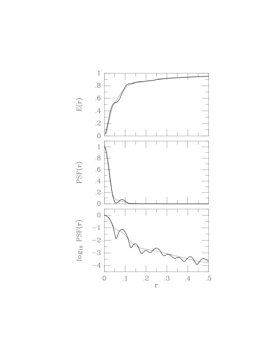
Figure 7: Heavy dotted curves are the results of calculations with the TinyTim software package for: (Top panel) $E(r)$, the encircled flux curve; (Middle panel) ${\rm PSF}(r)$ on a linear scale; and (Bottom panel) ${\rm PSF}(r)$ on a logarithmic scale. The thin solid curve shows the fit to these calculations obtained with the multi-Gaussian PSF model described in Section 3.5.

To constrain all the unknown parameters we used the measurements for ${\cal C}$ and ${\cal S}$, not only for the grand-total spectra as shown in Figure 3, but also for each of the rows in the individual two-dimensional spectra. While these constraints by themselves were sufficient to obtain acceptable results, we found that the calibration star data do not very accurately constrain the PSF at intermediate and large radii. To improve this situation we used a model estimate for ${\rm PSF}(r)$ as an additional constraint in the fit. For this, the TinyTim software was used to calculate the STIS PSF at the central wavelength of our observations. While this PSF is formally appropriate only for the STIS imaging mode, no better approximation for spectroscopy is readily available. The TinyTim PSF and its associated encircled flux curve are shown in Figure 7. Of course, addition of a model PSF as a constraint in the fit can make the results worse rather than better, if the model PSF is not in fact consistent with the calibration star data. We have found no evidence for this, and in fact, from a variety of tests we conclude that the two are fully consistent.

To determine the complete set of parameters in our multi-Gaussian PSF model that best fits all the combined constraints, we used a ‘downhill simplex’ minimization routine (Press et al. 1992). We found that adequate results were obtained with $N=5$ Gaussians in the multi-Gaussian PSF. The thin solid curves in Figures 6 and 7 shows the predictions of the best fitting model with this $N$. The parameters of the multi-Gaussian PSF are listed in Table 2.

3.6 Discussion

As has been discussed, there are many complications in the determination of stellar velocities with HST/STIS at the few km/s level: HST orbits the Earth as it exposes; the wavelength scale may drift during an orbit; and a wavelength shift is perceived for a star that is not perfectly centered in the slit. The most important result of the calibration star observations is therefore the data-model comparison shown in the bottom panel of Figure 6. The model predictions fit the observed wavelength shifts ${\cal S}$ with an RMS residual of $0.13$ pixels. This corresponds to $2.1\>{\rm km}\,{\rm s}^{-1}$. So if the position of a star with respect to the slit is known, then the observed line of sight velocity can be calibrated to this accuracy. Since the central velocity dispersion of M15 is $\sigma\approx 12\>{\rm km}\,{\rm s}^{-1}$, this accuracy is sufficient for the purposes of the present program. The excellent fit in the bottom panel of Figure 6 verifies not only our PSF and LSF modeling procedures, but also provides a stringent test of our data acquisition strategy and data reduction procedures.

Figure 7 shows that our multi-Gaussian PSF model is essentially a smooth fit to the true PSF. Computational convenience is gained, but some of the intricate detail of the PSF is lost. Most noticeably, the multi-Gaussian PSF does not reproduce the first Airy ring of the PSF (see in particular the middle panel of Figure 7). However, this is no reason for great concern. To appreciate this, note that the PSF is itself a purely theoretical construct that is generally unobservable. What is observed is the convolution of the PSF with the response function of an individual pixel, denoted the ‘effective PSF’ (ePSF) by Anderson & King (2000). Due to the convolution with the pixel size, the Airy rings are much less pronounced in the ePSF than in the PSF. As a result, the ePSF of our model is much closer to the true ePSF, than is the PSF of our model to true PSF. In fact, the observable quantities of interest for this program are exactly those shown in Figure 6, and indeed, those are adequately reproduced by the model.

4 STIS Spectroscopy of M15

4.1 Observations

We obtained spectra of the central region of M15 for a period of 24 HST orbits, separated over 6 different visits. The first visit (5 orbits) was executed on October 21, 1999. Based on the analysis of the data from the first visit some minor modifications were made to the observing strategy. The remaining visits were then planned for the third week of May 2001. Indeed, the data for visit 2 (4 orbits) were obtained on May 15, 2001. However, on May 16, 2001, the primary (Side 1) set of STIS electronics failed, which took the instrument out of commission for two months. STIS was then revived using the redundant (Side 2) set. This did not affect the instrument characteristics in a major way, apart from a minor increase in the detector read-noise and a somewhat different dark count rate. The remaining visits 3–5 (4 orbits each) and 6 (3 orbits) executed between October 22–26, 2001.

A complete log of the observations is presented in Table 3. All observations were done with the same slit width and grating setting as described in Section 3. Exposures were taken at 18 different positions covering the central region of the cluster. Figure 8 shows the slit positions as they were commanded to the telescope. The accuracy with which the intended positioning was achieved is discussed in Section 4.3 below. For all observations the slit was aligned along position angle ${\rm PA}=26.65^{\circ}$ (measured from North over East). This PA was chosen to allow the most flexible scheduling of the observations, and is otherwise fairly arbitrary. At each slit position we obtained spectra for a total exposure time that ranged from 46 to 60 minutes. Three or four exposures were obtained per position. Individual exposures were dithered by 4 pixels along the slit, to allow removal of CCD defects during data reduction. In visit 1 we placed the central region of M15 near the center of the CCD. In subsequent visits we placed the central region near row 900 (out of 1024), to mitigate the loss of signal due to deteriorations in the CTE of the STIS/CCD. In no case did we apply on-chip rebinning in the spectral direction, given that the $15.86\>{\rm km}\,{\rm s}^{-1}$ size of a single pixel is already large compared to the M15 velocity dispersion. However, in the first visit we applied 2-pixel on-chip rebinning in the spatial direction (as for the calibration star observations discussed in Section 3) to minimize the read-noise component in the spectra. In subsequent visits we did not apply such on-chip rebinning, to minimize the effects of PSF undersampling in the spatial direction. The large majority of the orbits consisted of the same simple observational sequence: an arc lamp exposure, followed by three target exposures and then another arc lamp exposure. In the end, the spectra from all visits had sufficient quality to achieve the science goals of our program.

Blind pointings with HST are accurate only at the level of $\sim 0.5^{\prime\prime}$, due to the accuracy of the GSCS. To position the STIS slit on M15 with the required accuracy it is therefore necessary to perform a target acquisition. STIS target acquisitions work by centering on the brightest object in a $5^{\prime\prime}\times 5^{\prime\prime}$ field. To ensure that the target acquisition would not acquire the wrong target, we searched for a bright and relatively isolated star in M15. The cross in Figure 1 marks the spatial position of the star that was chosen (#27604 in the WFPC2 catalog). Its position in the $(x,y)$ coordinate system defined in Section 2.2 is $(-3.286^{\prime\prime},-39.344^{\prime\prime})$. Its position in the M15 CMD shown in Figure 2 is also indicated by a cross. Each visit started with an acquisition of this star, consisting of an ACQ acquisition procedure. In most visits we then slewed the telescope to the intended position near the center of M15 to take the spectra. However, in visits 1 and 6 we performed an additional ACQ/PEAK acquisition procedure (Leitherer et al. 2001) and obtained spectra of the acquisition star, before slewing to the center of M15. In visit 1 we also repeated this procedure at the end of the visit, to allow an independent check of the repeatability of the velocity measurements for this particular star. The positional accuracy of the target acquisitions and the slews is discussed in Section 4.3 below. We generally performed a target acquisition only at the beginning of the first orbit of each visit, and not in any of the subsequent orbits.

4.2 Data Reduction

The data reduction of the M15 spectra was similar to the reduction of the calibration star spectra discussed in Section 3.2, including the wavelength calibration using arc lamp spectra obtained in the same orbit, and the correction for the HST velocity during the observations. This yields for each slit position a single two-dimensional frame with a linear heliocentric wavelength scale along rows, and a linear spatial scale along columns.

One difference between the observations of M15 and those of the calibration star is that we obtained only two arc-lamp spectra per orbit for M15, as compared to five for the calibration star. We did some quantitative analysis to address to what extent this may affect the analysis. The arc lamp spectra show that there are drifts in the wavelength scale over the course of a visit. These drifts are generally smoothly varying, and are fairly well modeled as a linear function of time. In the worst case (visit 2) the drift was $1.3$ pixels over the 4 orbits of the visit. Because we do in fact take two arc-lamp spectra per orbit, we can correct for most of this. In the reduction of the M15 spectra we assume that the wavelength scale for a given exposure can be obtained by linear interpolation in time between the results for the nearest arc lamp spectra. To test the accuracy of this, we applied this same procedure to each of the arc-lamp spectra. This yields the difference between the actual wavelength scale and the one that is obtained by linear interpolation between the previous and the next arc-lamp exposure in the visit. The RMS difference for all arc lamp spectra was found to be $0.08$ pixels, which corresponds to only $1.3\>{\rm km}\,{\rm s}^{-1}$. This accuracy is sufficient for the purposes of the project, especially since other effects already set a lower limit to the velocity accuracy of $2.1\>{\rm km}\,{\rm s}^{-1}$ (cf. Section 3.6).

4.3 Slit Positioning Accuracy

For accurate velocity determination of an M15 star it is essential to know its position with respect to the slit. From the WFPC2 imaging we know where all the stars are on the sky (see Section 2). So the next step is to determine the exact positioning of the slits for all observations. For this we analyzed and modeled the observed intensity profiles along the slit. These essentially provide one-dimensional (linear) images of M15, which uniquely constrain the telescope pointing.

To model an observed intensity profile along the slit we proceed as follows. For each star in the WFPC2 catalog we use the observed Johnson B and V magnitudes to estimate the flux $F_{\nu}$ at 5216Å (the center of the wavelength range for the spectra). We choose a trial position of the slit on the sky. For each pixel along the slit we calculate the flux contributed by each star, using the formulae derived in Section 3.5. Adding the contributions of all stars in the catalog yields the predicted intensity profile along the slit for the given assumed slit position. This profile can be compared to the observed profile in a $\chi^{2}$ sense (using an arbitrary scaling that corresponds to the efficiency of the telescope+instrument system). Looping over a fine grid of possible slit positions yields the position with minimum $\chi^{2}$, which corresponds to the estimated position of the slit on the sky. To obtain adequate fits we found that we had to add a smooth, low-intensity model for the light contribution of faint stars that are missing from the WFPC2 catalog due to incompleteness. As an example of the procedure, Figure 9 shows the final data-model comparison for one of the slit positions.

The accuracy with which HST can achieve a requested roll angle is $\sim 0.003^{\circ}$. The accuracy with which the slit PA on the sky is known is dominated by the calibration uncertainty in the relative angle of the slit within the instrument, which is $\sim 0.05^{\circ}$. This is small enough that it can be neglected in the present context. We therefore did not include the slit PA as a free parameter in the fits to the intensity profiles, but kept it fixed at the value commanded to the telescope. To confirm the validity of this approach we did a number of test runs in which we fitted observed M15 intensity profiles with the slit PA treated as a free parameter. These tests indeed implied PA values consistent with the value commanded to the telescope, to within the quoted uncertainty.

The intensity profile modeling yields for each observation the actual pointing position of the telescope during the exposures. The intended pointings are known as well, so it is possible to determine for each observation the offset $(\Delta X,\Delta Y)$ of the actual pointing from the intended pointing. The results are shown in Figure 10. Observations from the same visit are shown with the same plot symbol. The offsets satisfy $|\Delta X|<0.1^{\prime\prime}$ and $|\Delta Y|<0.1^{\prime\prime}$ for all observations. These absolute pointing accuracies are not so important in the present context; the aim of the observational strategy was to scan the central region of M15, and not to point at any object in particular. However, it is important to know the accuracy of our determinations of $(\Delta X,\Delta Y)$. To this end we need to understand the sources of the inferred pointing offsets.

The first source of pointing error is the limited astrometric accuracy of the WFPC2 catalog. Figure 1 shows that the star that was used for target acquisitions was on a different CCD chip in the WFPC2 observations than the center of M15. The astrometric calibration of WFPC2 is considerably less accurate across CCD chips than within a given CCD chip ($0.1^{\prime\prime}$ as compared to $0.005^{\prime\prime}$, according to the HST Data Handbook; Voit et al. 1997). Since the slew that we applied from the acquisition star to the M15 center was based on the astrometry of our catalog, an error in this astrometry would yield a fixed non-zero component to the offsets $(\Delta X,\Delta Y)$ for all observations.

The second source of pointing error is the limited accuracy with which the positions of the apertures are known within the STIS instrument. An ACQ acquisition centers the target in the 0.2X0.2 aperture. On-board software then applies a telescope slew to place the target behind the science aperture (the 52X0.1 in the present case). If there is an error in the expected position of the science aperture, this yields a fixed non-zero pointing error relative to the slit. We obtained the data for visit 2 in a configuration that is rotated by $180^{\circ}$ with respect to that for the other visits. So any component in the offsets $(\Delta X,\Delta Y)$ due to this effect would have the opposite sign for visit 2 as compared to the other visits. Figure 1 shows that the average offset for visit 2 is $(-0.059^{\prime\prime},0.004^{\prime\prime})$, whereas the average for all the other visits is $(0.066^{\prime\prime},0.024^{\prime\prime})$. So there is indeed evidence for pointing errors of this nature.

The third source of pointing error is the limited accuracy of the target acquisitions that start each visit. For most visits we only used an ACQ acquisition procedure, and not the more accurate ACQ/PEAK procedure. The former has a nominal accuracy between $0.01^{\prime\prime}$ (Leitherer et al. 2001) and $0.025^{\prime\prime}$ (Voit et al. 1997).

The fourth source of pointing error is the limited accuracy of the $39.5^{\prime\prime}$ slews from the acquisition star to the M15 center. The nominal accuracy of such slews is $0.02^{\prime\prime}$ (Downes & Rose 2001).

The first four sources of error can explain both the size and the scatter in the pointing offsets for different visits. However, these error sources predict identical offsets for all observations in the same visit. In reality, there is some scatter among the pointing offsets for observations in the same visit, but this scatter is very small: $0.005^{\prime\prime}$ in the $X$ direction, and $0.007^{\prime\prime}$ in the $Y$ direction. We attribute this to the fifth source of pointing error: small pointing drifts during a visit as a result of thermal effects on the telescope (Downes & Rose 2001).

The small scatter in the offsets for observations in the same visit implies that our models for determining the slit positions from the data must be very accurate. The numerical accuracy can be no worse than $0.007^{\prime\prime}$ in each coordinate. An error of this size in the STIS $X$ coordinate corresponds to a wavelength shift $\Delta{\cal S}$ of at most $0.08$ pixels, cf. the bottom panel of Figure 6. This corresponds to $1.2\>{\rm km}\,{\rm s}^{-1}$. This accuracy is sufficient for the purposes of the project, especially since other effects already set a lower limit to the velocity accuracy of $2.1\>{\rm km}\,{\rm s}^{-1}$ (cf. Section 3.6).

5 Extraction of Spectra for Individual Stars

Each row in each of the 18 calibrated and rectified two-dimensional spectra contains the spectrum for a small aperture on the sky. From the analysis in Section 4.3, the positions of these apertures are known with a (two-dimensional) accuracy better than $0.01^{\prime\prime}$. Figure 11 shows the inferred aperture positionings for the central region of M15. In total there are 19,200 spectra in the dataset. Most spectra contain very little signal from any star, and are therefore of little use in the analysis. However, some spectra do contain considerable signal from one or more M15 stars. Many stars contribute significantly to more than one aperture. For proper analysis we therefore developed an algorithm to extract the spectra of individual stars.

The algorithm starts with the same modeling procedure used in Sections 3.5 and 4.3. From the known positions of all apertures $i$ and all stars $j$ we calculate predictions for three sets of quantities: (i) $F_{i}$, the total flux observed in an aperture $i$; (ii) $F_{ij}$, the total flux contributed by star $j$ to aperture $i$; and (iii) ${\cal S}_{ij}$, the velocity offset with which star $j$ contributes flux to aperture $i$. Let $F_{j}$ be the total flux of star $j$. We define $g_{ij}=F_{ij}/F_{j}$ to be the fraction of the flux of star $j$ that falls in aperture $i$. We also define $f_{ij}\equiv F_{ij}/F_{i}$ to be the fraction of the total flux in aperture $i$ that is contributed by star $j$. For each aperture $i$ there is one star $j$ in the catalog for which $f_{ij}$ has the largest value. We denote the index number of this star as $J(i)$. We denote an aperture as ‘usable’ if the following three statements are true: (i) $f_{iJ(i)}\geq 0.5$ (i.e., there is a single star that contributes at least half of all the flux in the aperture); (ii) $F_{iJ(i)}\geq 6.3\times 10^{-18}\>{\rm erg}\>{\rm cm}^{-2}\>{\rm s}^{-1}\>{\rm\AA}^{-1}$ (i.e., there is a non-negligible amount of flux from this star in the aperture; this limit corresponds to a $V$-band magnitude of $\sim 22$); and (iii) $g_{iJ(i)}\geq 0.005$ (the aperture contains a non-negligible fraction of the total flux of this star). Apertures that are not usable are ignored in all of the subsequent analysis. For each star $j$ we then make a list of all the apertures $i$ for which $J(i)=j$. Let $N(j)$ be the number of apertures for which this is the case. We denote a star to be ‘significant’ for our study if $N(j)>0$. We call the spectra for the usable apertures that make up $N(j)$ the ‘usable’ spectra for star $j$.

In the full dataset there are 1741 usable spectra for 636 significant stars. The goal is to combine the $N(j)$ usable spectra for each significant star $j$ into a final spectrum for that star. This can be done by taking the exposure-time weighted average of the usable spectra. However, there is the possibility to include or exclude each usable spectrum in or from the average, so there are $2^{N(j)}$ possible combinations to do the averaging. Specifically, one does not want to include spectra whose main effect is to increase the amount of noise or blending in the average. We developed an algorithm to optimize the quality of the final spectrum. The STIS data reduction pipeline creates an error frame for each spectrum. We use the data frames and the error frames to calculate for each usable spectrum the median flux $Z_{ij}$ from the star (i.e., the median observed flux multiplied by $f_{ij}$) and the median noise. From these quantities we calculate the signal-to-noise ratio $S/N$ for all of the $2^{N(j)}$ possible combinations of spectra. We also calculate for all combinations the fraction $h$ of the total flux in the averaged spectrum that is due to the significant star. We rejected all combinations in which $h$ is smaller than some value $h_{\rm min}$. Of the remaining combinations we adopt the one that produces the highest $S/N$. The instrumental velocity shift ${\cal S}_{j}$ of the final average spectrum of star $j$ is calculated as the weighted average of the ${\cal S}_{ij}$ for the apertures $i$ that are used in the combination; the weighting is done using the product of exposure time and the flux $Z_{ij}$.

We adopted $h_{\rm min}=0.75$ in the extraction, to ensure that the fraction of the flux in the final spectrum that is blended in from other stars is less than 25%. For the spectra to be useful for kinematical analysis they must have a sufficient $S/N$. As demonstrated in Paper II, an average $S/N\geq 5.5$ per pixel is a minimum requirement (although not a sufficient requirement) to obtain meaningful line-of-sight velocity measurements. All extracted spectra that did not satisfy this requirement were discarded. This ultimately yielded ‘acceptable’ spectra for 131 stars, out of which 15 stars are within $1^{\prime\prime}$ from the cluster center, 39 stars are within $2^{\prime\prime}$, and 87 stars are within $5^{\prime\prime}$.

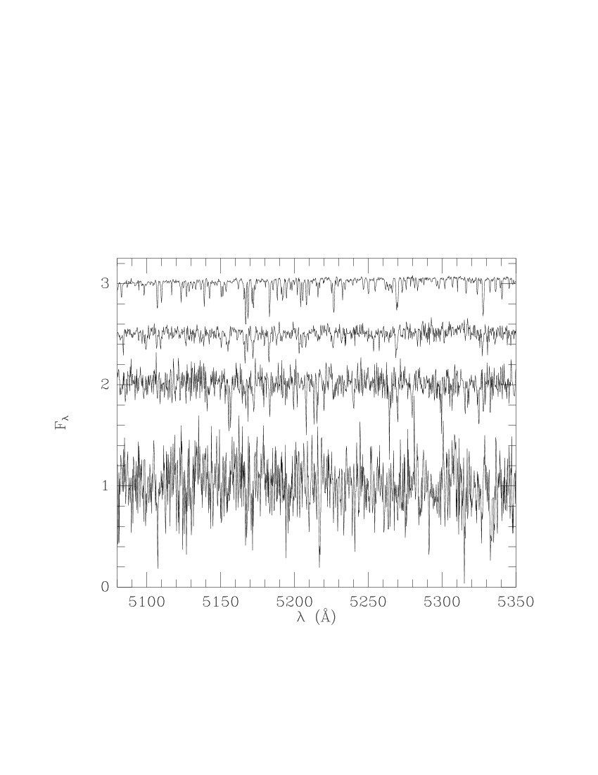
Figure 12: Four HST/STIS spectra of M15 giants in our final sample of 131 stars. The IDs of the stars in our WFPC2 Catalog are, from top to bottom: #6290 (magnitude $V=13.74$, color $B-V=1.01$, average $S/N=126.1$ per pixel); #6833 ($V=15.88$, $B-V=0.85$, $S/N=43.3$); #8396 ($V=17.31$, $B-V=0.68$, $S/N=18.7$); and #10589 ($V=18.10$, $B-V=0.64$, $S/N=7.3$). Although the bottom spectrum is quite noisy, the Mg b triplet lines at $\sim 5170$Å are still clearly visible. All spectra were normalized before plotting. For clarity, the top three spectra were offset vertically by $1$, $1.5$ and $2$ units, respectively.

Figure 12 shows the spectra for four stars in the final sample. All four spectra correspond to stars on the giant branch. From top to bottom, the $V$ magnitudes range from $V=13.74$ to $V=18.10$ while the average $S/N$ per pixel ranges from $126.1$ to $7.3$. Although the bottom spectrum is quite noisy, the Mg b triplet lines at $\sim 5170$Å are still clearly visible. The faintest star for which we were able to extract a spectrum with $S/N>5.5$ from the STIS data has magnitude $V=19.15$, which is just above the main sequence turnoff.

The spectra in Figure 12 are all reasonably ‘flat’, and do not show the undulations seen in Figure 4. This is because the spectra are sums of individual apertures for several slit positions. Each of the individual spectra has undulations, but these tend to cancel in the final co-addition. Approximately 10 per cent of the stars in our final list of 131 are based on only a single aperture. The final spectra for these stars show undulations similar to those in Figure 4. As explained in Section 3.3, this does not compromise our ability to infer radial velocities for these stars.

The 131 individual stellar spectra that we extracted from the STIS data form the end product of the present paper. It is shown in Paper II that accurate velocities can be determined for 64 of these stars. The spatial and color-magnitude distributions of these stars are discussed in Paper II. That paper also discussed the implications of the inferred velocities for our understanding of the structure and kinematics of M15.

6 Conclusions

The globular cluster M15 is one of the densest globular clusters in our Galaxy. A variety of interesting dynamical and structural evolutionary phenomena have been predicted to occur at high stellar densities, including mass segregation and the possible formation of a central black hole. Stellar kinematical data are required required to address these issues observationally. While M15 has been one of the globular clusters that has been most intensively studied in the past decades, ground-based data have only been able to provide limited information in the central few arcsec. We therefore executed a project to map the center of M15 spectroscopically at high spatial resolution with HST/STIS.

Our observational project is at the limit of what is feasible with HST/STIS. The pixel size of our spectra corresponds to $15.86\>{\rm km}\,{\rm s}^{-1}$, which exceeds the central velocity dispersion of M15 ($\sim 12\>{\rm km}\,{\rm s}^{-1}$; Gebhardt et al. 2000a). Extreme care therefore had to be taken in the reduction and velocity calibration of the data. The main result of the present paper is that we have in fact succeeded in extracting accurately calibrated spectra from our data. The implications of this for our understanding of M15 are discussed in Paper II.

To be able to properly interpret the long-slit spectra, we started by creating a stellar catalog for M15. We used the HST/WFPC2 data discussed previously by G96, but we performed an improved astrometric and photometric calibration. The final stellar catalog contains 31,983 stars with their positions and U, B and V magnitudes. It is spatially complete within $14.9^{\prime\prime}$ from the cluster center, and extends as far as $2.0$ arcmin from the cluster center in some directions. The catalog contains stars down to magnitude $V\approx 22.5$, and it is photometrically complete for stars brighter than $V\approx 19$.

For proper calibration of the M15 spectra we performed a set of observations of a bright field star, with the star placed at various positions with respect to the slit. After basic data reduction and correction for the velocity of HST around the Earth we used these spectra for modeling the PSF and LSF of STIS. This is particularly important for understanding the apparent velocity shift for a star that is offset from the center of the slit. We derive a simple multi-Gaussian model for the PSF that reproduces the observed shifts with an RMS residual of only $2.1\>{\rm km}\,{\rm s}^{-1}$ (for a known stellar position with respect to the slit). Spatial undersampling causes artificial undulations in the spectra, but this only affects low frequencies and does not affect the determination of radial velocities through cross-correlation.

The M15 observations consisted of 6 HST visits spread over 2 years. The central region of the cluster was ‘scanned’ by consecutively placing the $0.1^{\prime\prime}$ slit at 18 adjacent positions. The intensity profiles along the slits were used to accurately determine the actual slit positions on the sky. With use of our WFPC2 catalog and PSF model we find that these positions can be determined to an accuracy of $0.007^{\prime\prime}$ in each coordinate. Positional errors in our knowledge of the slit positions translate directly into velocity errors, but with the achieved positional accuracy these errors are no larger than $1.2\>{\rm km}\,{\rm s}^{-1}$.

The reduced and calibrated data set contains 19,200 STIS spectra, each for a different aperture position in M15. We developed an algorithm that co-adds the spectra for individual apertures, so as to extract spectra of individual stars with minimum blending and maximum $S/N$. Our data allowed us to extract spectra with an average $S/N>5.5$ per pixel for a total of 131 stars, out of which 15 stars are within $1^{\prime\prime}$ from the cluster center, 39 stars are within $2^{\prime\prime}$, and 87 stars are within $5^{\prime\prime}$. In Paper II we show that reliable line-of-sight velocities can be derived for 64 of these stars, and that this provides enough new information to significantly improve our understanding of the dynamics and structure of M15.

Figure 3: Schematic illustration of the setup for the spectroscopic observations of the calibration star HD 122563. The STIS $X$ direction is perpendicular to the slit, and the $Y$ direction is along the slit. Note that the three panels are offset from each other by $2^{\prime\prime}$ in $Y$. The grating disperses the light that falls through the slit such that wavelength increases in the positive $X$ direction. The origin of the coordinate system is defined as the position of the star after the target acquisition procedure. The symbols denote the 14 different positions relative to this origin at which the star was subsequently placed using small telescope slews. At each position two exposures were taken which were co-added during data reduction. The bold dotted lines indicate the positions of the slit and the CCD pixels along the slit, as determined from the data (see Section 3.5). Note that the slit was not centered on the line $X=0$, i.e., the star was not perfectly centered in the slit after the target acquisition procedure.

Figure 4: HST/STIS spectra of the calibration star HD 122563. Top curve: a rectified 2D spectrum summed along all rows. Bottom curve: the brightest row of the same rectified 2D spectrum. Both spectra were normalized before plotting; for clarity, the top spectrum was offset vertically by $1$ unit. Due to spatial undersampling, the individual rows of 2D rectified STIS spectra show low-frequency undulations multiplied into the spectrum. Due to their low-frequency, these undulations do not compromise our ability to measure radial velocities using cross-correlation techniques (see Figure 5).

Figure 5: The cross-correlation function $f_{\rm cc}$ of the two spectra shown in Figure 4, as function of the applied shift $\Delta V$ (in $\>{\rm km}\,{\rm s}^{-1}$). The bottom curve shows the result without any continuum-subtraction or low-frequency filtering. There is a narrow peak at $\Delta V=0$ (the correct value), but there are secondary peaks of almost equal amplitude due to the low-frequency undulations in one of the two spectra. The top curve shows the result when continuum-subtraction and low-frequency filtering are applied as recommended in cross-correlation techniques (Tonry & Davies 1979); for clarity, the top curve was offset vertically by $1$ unit. The peak at $\Delta V=0$ is now unmistakable. This illustrates that velocity determinations are not adversely affected by the low-frequency undulations in the observed spectra.

Figure 6: Analysis of the calibration star observations. Each data point corresponds to a fixed position of the star with respect to the slit. The quantity $X$ along the abscissa is the position of the star in the direction perpendicular to the slit. The symbols and coordinate system are the same as in Figure 3. A single grand-total one-dimensional spectrum was constructed for each position of the calibration star, by co-adding all rows in the reduced two-dimensional frame. The quantity ${\cal C}$ shown in the top panel is the count-rate in the grand-total spectrum, in arbitrary units. The quantity ${\cal S}$ shown in the bottom panel is the wavelength shift ${\cal S}$ (in pixels) of the grand-total spectrum with respect to a fixed arbitrary standard. The solid curves show the fit to these data obtained with the multi-Gaussian PSF model described in Section 3.5. The vertical dotted line shows the inferred value $X_{\rm slit}$ of the slit center (see also Figure 3). The horizontal dotted line is the model value ${\cal S}={\cal S}_{\rm slit}$ at the slit center.

Figure 8: Schematic diagram of the central $2.5^{\prime\prime}\times 2.5^{\prime\prime}$ of M15. The orientation and coordinate system are as in Figure 1. The origin is at the position of the cluster center determined by G96, which has a 1-$\sigma$ uncertainty of $0.2^{\prime\prime}$ in each coordinate. The corresponding two-dimensional $68.3$% and $95.4$% confidence regions on the cluster center are shown as a solid and a dotted circle, respectively. All the stars in the WFPC2 catalog that are brighter than $V=20$ are shown; brighter stars are indicated with slightly larger symbols. HST/STIS observations were obtained at 18 different slit positions with a slit width of $0.095^{\prime\prime}$. The slit positions are displayed as they were commanded to the telescope. The actual achieved slit positionings were slightly different, as discussed in Section 4.3.

Figure 9: The intensity profile along the slit for one of the observations. The solid curve shows the flux observed in each row of the calibrated and rectified two-dimensional frame, averaged over the full wavelength range of the spectrum. Each row corresponds to $0.05071^{\prime\prime}$. The dashed curve shows the predictions of the best fit model, obtained as described in Section 4.3. The model is based on the WFPC2 stellar catalog described in Section 2 and the PSF model described in Section 3.5. It also includes a smooth model for the light contribution of faint stars that are missing from the WFPC2 catalog due to incompleteness (dotted curve). [For reference, the intensity profile corresponds to the third slit from the right in Figure 11. Rownumbers increase towards the top left in that figure; the peak at row 930 is due to star #7313 in the WFPC2 Catalog, at position $(x,y)=(2.021^{\prime\prime},-2.193^{\prime\prime})$.].

Figure 10: Positional differences $(\Delta X,\Delta Y)$ between the expected pointing of the telescope (as commanded during scheduling), and the actual pointing of the telescope (determined from intensity profile modeling as in Figure 9). The 18 symbols correspond to the 18 slit positions shown in Figure 8. Observations indicated with the same plot symbol were obtained in the same visit (Visit 1: filled circles; Visit 2: open circles; Visit 3: open squares; Visit 4: open triangles; Visit 5: filled squares; and Visit 6: asterisks). The STIS $X$ direction is perpendicular to the slit, and the $Y$ direction is along the slit.

Figure 11: Schematic diagram of the central $2.5^{\prime\prime}\times 2.5^{\prime\prime}$ of M15, as in Figure 8. The indicated slit and pixel positions are those that were actually achieved during the HST/STIS observations. The positions were calculated from the observed intensity profiles along the slits (see Section 4.3), and are accurate to better than $0.01^{\prime\prime}$. The coverage of the central region of M15 was not quite as homogeneous as planned (compare to Figure 8) due to small pointing errors (see Figure 10).

Table 1: HST/WFPC2 Photometric Catalog of M15

ID	$\Delta{\rm RA}$	$\Delta{\rm DEC}$	$V$	$B$	$U$
	(arcsec)	(arcsec)
(1)	(2)	(3)	(4)	(5)	(6)
1	16.343	10.269	20.467	21.313	20.869
2	18.180	8.384	20.889	21.701	21.624
3	7.251	19.504	20.271	20.900	20.623
4	18.725	7.807	19.363	19.893	19.738
5	2.529	24.193	20.256	20.583	20.534
6	2.170	24.551	20.325	20.994	20.738
7	17.248	9.263	20.738	21.234	21.206
8	11.883	14.729	14.659	15.562	15.894
9	1.843	24.853	20.619	21.485	21.278
10	15.338	11.195	19.454	19.935	19.840
11	22.580	3.733	20.957	21.767	21.958
12	19.811	6.584	18.549	19.215	19.148
13	6.533	20.103	19.973	20.440	20.372
14	3.334	23.280	20.557	21.253	20.911
15	16.777	9.611	20.453	21.105	20.926
16	3.759	22.784	20.885	21.633	21.377
17	8.709	17.789	20.776	21.377	21.155
18	13.186	13.240	20.985	22.073	21.703
19	8.817	17.666	19.188	19.698	19.478
20	21.074	5.129	19.719	20.445	20.145
21	4.649	21.815	20.424	20.885	20.718
22	6.399	20.045	20.568	21.132	20.988
23	20.324	5.839	20.359	21.056	20.829
24	6.592	19.834	19.828	20.382	20.294
25	16.308	9.954	20.307	21.043	20.993

Note. — First 25 entries of the HST/WFPC2 photometric catalog described in Section 2.3. The full catalog contains 31,983 stars and is distributed electronically as part of this paper. Column (1) is the ID number of the star. Columns (2) and (3) give positions $({\rm RA},{\rm DEC})$ of each star, measured with respect to the M15 cluster center as described in Section 2.2. Columns (4), (5) and (6) give the broad-band $V$, $B$ and $U$ magnitudes of the stars.

Table 2: Multi-Gaussian PSF model parameters

$i$	$\gamma_{i}$	$\sigma_{i}$
		(arcsec)
1	$0.589$	$0.020$
2	$-0.625$	$0.032$
3	$0.836$	$0.044$
4	$0.129$	$0.165$
5	$0.071$	$0.572$

Note. — The listed parameters describe the multi-Gaussian PSF model, defined by equation (1), that was used for the analysis and interpretation of the M15 spectroscopy. The PSF model provides the optimum fit to the combined data shown in Figures 6 and 7, as described in Section 3.5.

Table 3: M15 STIS Observations: Observation Log

position	$T_{\rm exp}$	$N_{\rm exp}$	rebin	visit
(arcsec)	(sec)
(1)	(2)	(3)	(4)	(5)
$+0.6$	2862	4	1	6
$+0.5$	2790	4	2	1
$+0.4$	2760	3	2	1
$+0.3$	2760	3	2	1
$+0.2$	2760	3	2	1
$+0.1$	3113	4	1	2
$+0.0$	3578	4	1	2
$-0.1$	3556	4	1	2
$-0.2$	3113	4	1	3
$-0.3$	3578	4	1	3
$-0.4$	3556	4	1	3
$-0.5$	3113	4	1	4
$-0.6$	3578	4	1	4
$-0.7$	3556	4	1	4
$-0.8$	3113	4	1	5
$-0.9$	3578	4	1	5
$-1.0$	3556	4	1	5
$-1.1$	3554	4	1	6

Note. — All observations were taken with the 52X0.1 slit along position angle ${\rm PA}=26.65^{\circ}$ on the sky, measured from North over East. Column (1) lists the offset of the slit from the M15 center, measured in the direction of position angle PA=$116.65^{\circ}$. The listed offset is the one that was commanded to the telescope; the actual offsets as determined from the data are slightly different, as described in Section 4.3. The position of the M15 center was chosen as described in Section 2.2. Column (2) lists the total exposure time at the given slit position. Column (3) lists the number of exposures. Column (4) lists the number of spatial pixels that were rebinned ‘on-chip’ during CCD read-out. Column (5) lists the number of the visit in which the observations were done.

References

- (1) Anderson, J., & King, I. R. 2000, PASP, 112, 1360
- (2) Bahcall, J. N., & Wolf R. A. 1976, ApJ, 209, 214
- (3) Bahcall, J. N., & Wolf R. A. 1977, ApJ, 216, 883
- (4) Biretta, J., et al. 2001, WFPC2 Instrument Handbook, Version 6.0 (Baltimore: STScI)
- (5) Bohlin, R., & Hartig, G. 1998, STIS Instrument Science Report 98-20 (Baltimore: STScI)
- (6) Bowers, C., & Baum, S. 1998, STIS Instrument Science Report 98-23 (Baltimore: STScI)
- (7) de Marchi, G., & Paresce, F. 1994, ApJ, 422, 597
- (8) de Marchi, G., & Paresce, F. 1996, ApJ, 467, 658
- (9) Downes, R., & Rose, S. 2001, HST Primer for Cycle 11 (Baltimore: STScI)
- (10) Drukier, G. A., Slavin, S. D., Cohn, H. N., Lugger, P. M., Berrington, R. C., Murphy, B. W., Seitzer, P. O. 1998, AJ, 115, 708
- (11) Dubath, P., & Meylan, G. 1994, A&A, 290, 104
- (12) Dubath, P., Meylan, G., & Mayor, M. 1994, ApJ, 426, 192
- (13) Dull, J. D., Cohn, H. N., Lugger, P. M., Murphy, B. W., Seitzer, P. O., Callanan, P. J., Rutten, R., Charles, P. 1997, ApJ, 481, 267
- (14) Durrell, P. R., & Harris, W. E. 1993, AJ, 105, 1420
- (15) Ferraro, F. R., & Paresce, F. 1993, AJ, 106, 154
- (16) Gebhardt, K., Pryor, C., Williams, T. B., Hesser, J. E., 1994, AJ, 107, 2067
- (17) Gebhardt, K., Pryor, C., Williams, T. B., Hesser, J. E., & Stetson, P. B. 1997, AJ, 113, 1026
- (18) Gebhardt, K., Pryor, C., O’Connell, R. D., Williams, T. B., & Hesser, J. E. 2000a, AJ, 119, 1268
- (19) Gerssen, J., van der Marel, R. P., Gebhardt, K., Guhathakurta, P., Peterson, R. C., & Pryor, C. 2002, AJ, submitted (Paper II)
- (20) Guhathakurta, P., Yanny, B., Schneider, D. P., & Bahcall, J. N., 1996, AJ, 111, 267 (G96)
- (21) Harris, W.E. 1996, AJ, 112, 1487
- (22) Holtzman, J., et al. 1995a, PASP, 107, 156
- (23) Holtzman, J., et al. 1995b, PASP, 107, 1065
- (24) Krist, J., & Hook, R. 2001, The Tiny Tim User’s Guide, Version 6.0 (Baltimore: STScI)
- (25) Kulkarni, S. R., Goss, W. M., Wolszczan, A., & Middleditch, J. 1990, ApJ, 363, L5
- (26) Leitherer, C., et al. 2001, STIS Instrument Handbook, Version 5.1, (Baltimore: STScI)
- (27) Peterson, R. C., Seitzer, P., & Cudworth, K. M. 1989, ApJ, 347, 251
- (28) Phinney, E. S. 1993, in Structure and Dynamics of Globular Clusters, eds., G. Djorgovski & G. Meylan, ASP Conference Series, Vol. 50, p. 141
- (29) Press, W. H., Teukolsky, S. A., Vetterling, W. T., & Flannery, B. P. 1992, Numerical Recipes (Cambridge: Cambridge University Press)
- (30) Rees, M. J. 1984, ARA&A, 22, 471
- (31) Stetson, P. B. 1994, PASP, 106, 250
- (32) Sosin, C., & King, I. R. 1997, AJ, 113, 1328
- (33) Tonry, J., & Davis, M. 1979, AJ, 84, 1511
- (34) van der Marel, R. P. 1995, in ‘Calibrating Hubble Space Telescope: Post Servicing Mission’, eds., A. Koratkar, & C. Leitherer (Baltimore: STScI), 94
- (35) van der Marel, R. P. 2001, in ‘Black Holes in Binaries and Galactic Nuclei’, Kaper L., van den Heuvel E. P. J., Woudt P. A., eds., Springer-Verlag, p. 246
- (36) van der Marel, R. P., de Zeeuw, P. T., & Rix H.-W. 1997, ApJ, 488, 119
- (37) Voit, M. 1997, HST Data Handbook, Vol. I, Current Instruments, Version 3 (Baltimore: STScI)
- (38) White, N. E., & Angelini, L. 2001, ApJ, 561, L101
- (39) Whitmore, B., & Heyer, I. 1997, WFPC2 Instrument Science Report 97-08 (Baltimore: STScI)
- (40) Yanny, B., Guhathakurta, P., Bahcall, J. N., & Schneider, D. P. 1994, AJ, 107, 1745
- (41) Zaggia, S. R., Capaccioli, M., Piotto, G., & Stiavelli M. 1992, A&A, 258, 302
- (42) Zaggia, S., Capaccioli, M., & Piotto, G. 1993, A&A, 278, 415