Gravitation of the Casimir Effect
and the Cosmological Non-Constant

Abstract

Whereas the total energy in zero-point fluctuations of the particle physics vacuum gives rise to the cosmological constant problem, differences in the vacuum give rise to real physical phenomena, such as the Casimir effect. Hence we consider the zero-point energy bound between two parallel conducting plates — proxy for a solid slice of cosmological constant — as a convenient laboratory in which to investigate the gravitation and inertia of vacuum energy. We calculate the Casimir effect in a weak gravitational field, obtaining corrections to the vacuum stress-energy and attractive force on the plates due to the curvature of spacetime. These results suggest that if the cosmological constant is due to zero-point energy then it is susceptible to fluctuations induced by gravitational sources.

The Casimir effect [1, 2] is one of the most remarkable phenomena in the strange and spooky world of quantum mechanics. At the most basic level, the attractive force acting on two parallel conducting plates is a physical manifestation of zero-point energy. Idealized, the plates are cold and uncharged in vacuo, so there are no real particles or fields present, but a virtual quantum electrodynamic field creates a pressure difference across the plates, resulting in this uniquely quantum force.

Our attraction to the Casimir effect follows from its potential relationship to the cosmological constant ($\Lambda$) [3, 4] — perhaps a cosmological manifestation of zero-point energy. In Zeldovich’s landmark 1968 paper [5] he declared that once Einstein has introduced $\Lambda$, “the genie has been let out of the bottle and it is no longer easy to force it back in.” In a prescient statement, he observed that “a new field of activity arises, namely the determination of $\Lambda$”: What is known about it? What are the limits on it? What experiments can probe $\Lambda$? Numerous experiments are currently focusing on these very questions! [6] Furthermore, Zeldovich offered the provocative suggestion that the cosmological constant may be due to the energy density and pressure of the particle physics vacuum. In support of this speculation, he used the energy density and pressure for the vacuum of scalar particles of mass $m$

$$\rho={\hbar c\over 2(2\pi)^{3}}\int_{0}^{\infty}\,d^{3}k\,\sqrt{k^{2}+(mc/\hbar)^{2}},\qquad p={\hbar c\over 6(2\pi)^{3}}\int_{0}^{\infty}\,d^{3}k\,{k^{2}\over\sqrt{k^{2}+(mc/\hbar)^{2}}}$$ (1)

and showed that the regularized stress-energy has the form of Einstein’s constant, whereby $p_{\Lambda}=-\rho_{\Lambda}$. In this paper we take our lead from Zeldovich, and investigate how the virtual quanta of the vacuum of a scalar field mixes with gravity.

Where can we find a handful of vacuum energy to analyze in the laboratory? The reality of zero-point fluctuation forces is firmly established, considering the dramatic progress which has been made in the measurement of the Casimir effect in recent years. In fact, the Casimir effect for parallel plates has just recently been measured, by Bressi and collaborators [7]. (For an extensive review, see Ref. [8].) Hence, we will use this grounded phenomenon as the basis of our investigation, and conduct “theoretical experiments” to determine the response of the Casimir effect to a weak gravitational field.

We may choose from a variety of methods for calculating the Casimir energy of parallel plates in Minkowski spacetime, to use as a starting point. We follow the method described by Milton in Ref. [9], wherein the stress-energy is obtained from the vacuum expectation values of the electromagnetic field. In our calculation, however, we will substitute two free, minimally coupled scalar fields for the two polarization states of the electromagnetic field. One scalar field satisfies Dirichlet boundary conditions at the surface of the plates, whereas the other satisfies Neumann boundary conditions — in this way the requirements $\hat{n}\times\vec{E}=0$ and $\hat{n}\cdot\vec{B}=0$ for the electric and magnetic field on each plate are met, where $\hat{n}$ is a unit normal. For the parallel plate geometry, we expect our scalar field results to apply to the electromagnetic field. The central object of our calculation then is the scalar Feynman Green’s function, satisfying $\Box_{x}{\rm G}(x,x^{\prime})=-\delta(x,x^{\prime})$, which relates to the time-ordered scalar field vacuum expectation value $\langle\phi(x)\phi(x^{\prime})\rangle=-i\hbar{\rm G}(x,x^{\prime})$.

In the presence of a gravitational field, the Green’s function must satisfy $\Box_{x}{\rm G}(x,x^{\prime})=-\delta(x,x^{\prime})/\sqrt{-g}$. Rather than attempt an exact solution for a given spacetime, we seek an approximate solution which incorporates the leading-order effects of gravity. In this case, we use the line-element

$$ds^{2}=-(1-\epsilon\,{2{G}M\over r})dt^{2}+(1+\epsilon\,{2{G}M\over r})d\vec{x}^{2}$$ (2)

to describe the weak gravitational field in the vicinity of a mass $M$, as a perturbation to Minkowski spacetime. We put the plates at the origin of the coordinate system, and place the mass at a distance $R$, such that ${G}M/R\ll 1$. It is not necessary to assume that the distance between the plates, $a$, is small compared to $R$, but we do require that the mass lies outside the plates. Next, we expand all the terms in the Green’s function equation in powers of $\epsilon$, a dimensionless parameter which measures the strength of the gravitational field, including the Green’s function: ${\rm G}(x,x^{\prime})={\rm G}^{(0)}(x,x^{\prime})+\epsilon{\rm G}^{(1)}(x,x^{\prime})+{\cal O}(\epsilon^{2})$. The superscript indicates the perturbation order. Matching powers of $\epsilon$, the resultant equations are

$$\Box_{x}^{(0)}{\rm G}^{(0)}(x,x^{\prime})=-\delta(x,x^{\prime}),$$ (3)

$$\Box_{x}^{(0)}{\rm G}^{(1)}(x,x^{\prime})-{2{G}M\over r}(\partial_{t}^{2}+\nabla_{x}^{2}){\rm G}^{(0)}(x,x^{\prime})={2{G}M\over r}\delta(x,x^{\prime}).$$ (4)

We can use the properties of ${\rm G}^{(0)}$ to obtain a solution for ${\rm G}^{(1)}$:

$${\rm G}^{(1)}(x,x^{\prime\prime})=-\int d^{4}x^{\prime}\,{\rm G}^{(0)}(x,x^{\prime})\,{4{G}M\over r^{\prime}}{\partial_{t^{\prime}}^{2}}\,{\rm G}^{(0)}(x^{\prime},x^{\prime\prime}),$$ (5)

where ${\rm G}^{(0)}$ is the appropriate Green’s function for the unperturbed case, reflecting the boundary conditions enforced at the conducting plates.

The orientation of the conducting plates in the gravitational field is shown in Figure 1. The distance $r^{\prime}$ appearing in ${\rm G}^{(1)}$ is the distance between a point $\vec{x}^{\prime}$ and the mass at $(R\sin\theta,\,0,\,-R\cos\theta)$. Since the integral in equation (5) is dominated by the contribution between the plates, any orientation dependence enters at order ${\cal O}({G}M/R^{2})$, consistent with our use of the isotropic metric (2), the weak-field limit of Schwarzschild. (This answers the speculation [10] on an order ${\cal O}({G}M/R)$ orientation-dependence correction to the Casimir effect in the negative.)

Continuing, the Green’s functions are

$${\rm G}^{(0)}(x,x^{\prime}) = \int{d\omega\over 2\pi}\,{d^{2}k\over(2\pi)^{2}}\,{\rm e}^{-i\omega(t-t^{\prime})+i\vec{k}\cdot(\vec{x}-\vec{x}^{\prime})_{\perp}}\,g(z,z^{\prime})_{D,N}$$ (6)

$$g(z,z^{\prime})_{D} = \cases{{\sin\lambda(\frac{a}{2}+z_{<})\sin\lambda(\frac{a}{2}-z_{>})\over\lambda\sin\lambda a}&$-\frac{a}{2}<z,z^{\prime}<\frac{a}{2}$\cr{1\over\lambda}\sin\lambda(z_{<}-\frac{a}{2}){\rm e}^{i\lambda(z_{>}-\frac{a}{2})}&$\frac{a}{2}<z,z^{\prime}$}$$ (7)

$$g(z,z^{\prime})_{N} = \cases{-{\cos\lambda(\frac{a}{2}+z_{<})\cos\lambda(\frac{a}{2}-z_{>})\over\lambda\sin\lambda a}&$-\frac{a}{2}<z,z^{\prime}<\frac{a}{2}$\cr{i\over\lambda}\cos\lambda(z_{<}-\frac{a}{2}){\rm e}^{i\lambda(z_{>}-\frac{a}{2})}&$\frac{a}{2}<z,z^{\prime}$}$$ (9)

where the subscript $D,\,N$ indicates Dirichlet or Neumann, and $\lambda^{2}=w^{2}-k^{2}$. In the absence of the plates, $g(z,z^{\prime})=i{\rm e}^{i\lambda(z_{>}-z_{<})}/2\lambda$ for all $z,\,z^{\prime}$. Of course, these are the same reduced Green’s functions used for classical electrodynamics (for example, see Ref. [11]), but we will evaluate ${\rm G}^{(0)},\,{\rm G}^{(1)}$ by a complex integration which follows the path appropriate for the Feynman Green’s function. Finally, the stress-energy tensor is

$$\langle T_{\mu\nu}\rangle=\lim_{x^{\prime}\to x}\,\,\left[\partial_{\mu}\partial_{\nu^{\prime}}-\frac{1}{2}g_{\mu\nu}\,\partial_{\lambda}\partial^{\lambda^{\prime}}\right]\langle\phi(x)\phi(x^{\prime})\rangle.$$ (10)

Thus, we have all the tools necessary to compute the Casimir force and energy.

First, the Casimir force on the plate located at $z=\frac{a}{2}$ is obtained by evaluating the difference in radiation pressure on either side, at $z=\frac{a}{2}^{-}$ and $z=\frac{a}{2}^{+}$. In this way, there is no need to subtract off an infinite contribution by the background. Taking the stress-energy tensor and projecting along the unit spacelike normal $\hat{z}^{\alpha}=(0,0,0,1/\sqrt{g_{zz}})$, then the force per unit area $A$ acting on the plate is finally obtained as

$${F\over A}=\left[\hat{z}^{\alpha}\hat{z}^{\beta}\langle T_{\alpha\beta}\rangle\right]^{z\to\frac{a}{2}^{-}}_{z\to\frac{a}{2}^{+}} = -{\hbar c\pi^{2}\over 240{a_{p}}^{4}}\times\left\{1+{{G}M\over R}\left[{2a_{p}\over 3R}\cos\theta-{x_{p}a_{p}\over R^{2}}\sin 2\theta\right.\right.$$ (13)

$$\left.\left.+{2{a_{p}}^{2}(15-\pi^{2})\over 9\pi^{2}R^{2}}(1+3\cos 2\theta)+{\cal O}({\vec{x}_{p}\over R})^{3}\right]+{\cal O}({{G}M\over R})^{2}\right\}.$$

The subscript $p$ indicates proper length, so $a_{p}=\int_{-a/2}^{a/2}dz\sqrt{g_{zz}}$. We have included both the Dirichlet and Neumann fields, which contribute equally. For our first result, we find that the attractive force of the vacuum pressure is modified by the presence of the gravitational field, with correction terms proportional to the curvature: components of the Riemann curvature are proportional to ${G}M/R^{3}$, e.g. $R_{tztz}=-\frac{1}{2}(1+3\cos 2\theta){G}M/R^{3}$. For $\theta=0$ the force is enhanced, whereas for $\theta=\pi/2$ the magnitude of the force is weakened. Hence, the pressure of vacuum energy responds to variations in the neighboring gravitational field.

Second, the Casimir energy is obtained by projecting the stress-energy tensor along the unit timelike vector $\hat{t}^{\alpha}=(1/\sqrt{|g_{tt}|},0,0,0)$ and integrating over the volume between the plates. In this case, we must subtract the energy density in the absence of the plates, as well as remove unphysical, divergent contact terms due to the presence of the plates. (See Refs. [12, 13].) It is interesting to note that the Dirichlet and Neumann contact terms cancel to ${\cal O}({G}M/R)$. This cancellation does not carry over to higher order terms. However, if we consider the alternative stress-energy tensor ${\widetilde{T}}_{\mu\nu}=-\phi\nabla_{\mu}\nabla_{\nu}\phi+\frac{1}{2}g_{\mu\nu}\phi\Box\phi$, which differs from the standard form by surface terms, then we can use a linear combination of $T,\,{\widetilde{T}}$ to eliminate the unphysical, diverging contact terms. In this way, the stress-energy tensor is found to be

$$\langle{T^{\alpha}}_{\beta}\rangle = {\hbar c\pi^{2}\over 720{a_{p}}^{4}}\left\{{\bf M}_{0}+{{G}M\over R}\times\right.$$ (18)

$$\left[{\bf M}_{1}\left({4z_{p}\over 5R}\cos\theta-{6x_{p}z_{p}\over 5R^{2}}\sin 2\theta+{a_{p}^{2}-3(z_{p}+\frac{a_{p}}{2})^{2}\over 15R^{2}}{(1+3\cos 2\theta)}\right)\right.$$

$$\left.\left.+{\bf M}_{2}{a_{p}^{2}\over R^{2}}{1\over\pi^{2}}+{\bf M}_{3}{a_{p}^{2}\over R^{2}}{\cos 2\theta\over\pi^{2}}+{\bf\Pi}{3\over 10}{(a_{p}^{2}-4z_{p}^{2})\over R^{2}}\sin 2\theta\right]\right\}$$

where the diagonal matrices are ${\bf M}_{0}={\rm diag}(-1,1,1,-3)$, ${\bf M}_{1}={\rm diag}(1,3,3,-5)$, ${\bf M}_{2}={\rm diag}(-3,8,-13,-10)$, ${\bf M}_{3}={\rm diag}(-9,-18,3,-30)$, and the anisotropic term is ${\bf\Pi}|^{x}_{z}={\bf\Pi}|^{z}_{x}=1$, ${\bf\Pi}=0$ otherwise. The ${\bf M}_{0}$ term above is consistent with the results for the QED stress-energy tensor derived by Brown & Maclay [14] using the symmetries of the electromagnetic vacuum state in the presence of the conducting plates, to the extent that we use the proper plate separation, $a_{p}$, in the absence of curvature or finite-size effects (also see [15]). The above stress-energy tensor (18) is covariantly conserved, ${T^{\mu}}_{\nu;\mu}=0$. However, ${\bf M}_{2,3}$ are not traceless, and the stress-energy acquires a trace

$$T=g^{\mu\nu}T_{\mu\nu}=-{\hbar c\over 60{a_{p}}^{4}}{{G}M\over R}\left[{a_{p}^{2}\over R^{2}}(1+3\cos 2\theta)+{\cal O}({\vec{x}_{p}\over R})^{3}\right]+{\cal O}({{G}M\over R})^{2}.$$ (19)

Whereas the symmetry of the plates and the boundary conditions keep the tree-level stress-energy tensor traceless for our minimally-coupled field, the presence of the gravitational field breaks the planar-symmetry. The curvature-induced distortions of the fields now serve as a source for further gravitation.

Third, the field energy stored in the Casimir plates is

$${\cal E} = \int d^{3}\Sigma\,\,\hat{t}^{\alpha}\hat{t}^{\beta}\langle T_{\alpha\beta}\rangle=\int(\sqrt{-g}/\sqrt{-g_{tt}})\,d^{3}x\,\hat{t}^{\alpha}\hat{t}^{\beta}\,\langle T_{\alpha\beta}\rangle$$ (20)

$$= -{\hbar c\pi^{2}\over 720{a_{p}}^{4}}(A_{p}a_{p})\left\{1+{{G}M\over R}\left[{{a_{p}}^{2}\over\pi^{2}R^{2}}(1+3\cos 2\theta)+{\cal O}({\vec{x}_{p}\over R})^{3}\right]+{\cal O}({{G}M\over R})^{2}\right\}.$$ (22)

Here, $d^{3}\Sigma$ is the 3-volume element for an observer with 4-velocity $\hat{t}^{\alpha}$ at fixed time, and the proper area $A_{p}$ is a circular disk in the x-y plane centered at the origin. We have included both the Dirichlet and Neumann fields. As with the force, the curvature enhances the energy stored in the plates for $\theta=0$, and diminishes the energy for $\theta=\pi/2$. Hence, the vacuum energy responds to variations in the neighboring gravitational field.

The weak gravitational field exerts a force on the Casimir plates, as well as the vacuum energy and pressure bound to the plates. Neglecting tidal forces, the plates themselves would fall as a rigid body along a geodesic towards the mass $M$. Focusing on the fields alone, as a theoretical experiment we may consider the force necessary to support the energy-momentum of the fields in the vicinity of the mass which we can interpret as the “weight of the vacuum”

$$w_{\rm C}=\hat{r}^{\alpha}f_{\alpha}=\hat{r}^{\alpha}\hat{t}^{\mu}(\int d^{3}\Sigma\,\hat{t}^{\beta}\,\langle T_{\alpha\beta}\rangle)_{;\mu}={\cal E}{{G}M\over R^{2}}\left[1-{{G}M\over R}+{\cal O}({{G}M\over R})^{2}\right].$$ (23)

Here, $f^{\alpha}$ is the 4-force which we have contracted with a unit 4-vector $\hat{r}$, pointing from the origin to the mass, $M$. (Because the leading term in the covariant derivative is already of order ${G}M/R^{2}$, we have included one more term in the weak field expansion of the metric, namely $g_{tt}=-1+2({G}M/r)-2({G}M/r)^{2}$, consistent with the Schwarzschild metric in isotropic coordinates. Hence, the expression above is the standard parametrized-post-Newtonian result [16].) For comparison, a point particle of mass $m$ has $f^{\alpha}=u^{\mu}{p^{\alpha}}_{;\mu}$ with $p^{\alpha}=mu^{\alpha}$, so the weight is identical to (23) with the substitution ${\cal E}\to m$. Of course, the acceleration is the same, but the weight is influenced by the orientation of the plates relative to the mass, due to the $\theta-$dependence in equation (22).

The vacuum energy would seem to be buoyant, since $w_{\rm C}<0$. If we regard the negative Casimir energy as a sort of particle with negative gravitational mass, we would playfully expect it to accelerate towards the mass $M$, which in turn would be gravitationally repelled by the Casimir particle. One particle chases the other. (See problem 13.20 of Ref. [17].) Although the conducting plates contribute a positive mass $m$ to the system, we might imagine very light plates for which $m+{\cal E}<0$, to maintain our negative mass object. Nevertheless, the strain required to oppose the Casimir force and keep the plates at a constant separation contributes an energy density at least as large as the pressure (assuming the mechanism holding the plates fixed is composed of a material which satisfies the weak energy condition), so that the net mass-energy is positive. The Casimir energy is a binding energy, after all. This recalls Misner and Putnam’s discussion of active gravitational mass [18]: although the energy density and pressure of the fields serve as a source of gravitation, via $\Box h_{\mu\nu}=-16\pi G(T_{\mu\nu}-\frac{1}{2}g_{\mu\nu}T)$, if the pressure is contained by non-gravitational means, then the associated tension must offset the pressure, so that for the isolated system the active gravitational mass and inertial mass are the same.

The distinction between gravitation and inertia brings us back to the first cosmological models in Einstein’s nascent Theory of General Relativity. On the one hand we have de Sitter’s world-model, wherein the cosmological spacetime is filled by a “world-matter” ($\Lambda$) responsible for inertia, whereas the sources of gravitation, stars and nebulae like massive particles moving in the fixed background, are to be considered as gravitational perturbations [19]. This may seem to be an apt description of a Universe dominated by an idealized, immutable, yet unphysical cosmological constant. On the other hand, Einstein had supposed that the sun and stars may be condensed “world-matter,” and that the world-matter itself may very well be inhomogeneous on small scales, approaching a constant density on sufficiently large scales [20]. We can readily apply Einstein’s description to our results for the Casimir vacuum field energy, as a proxy for a physically-motivated cosmological constant.

We still don’t know how to calculate $\Lambda$ from first principles, but if there does exist a finite $\Lambda$ arising from zero-point energy, then we should not expect it to be a true and immutable constant. Although the presence of a boundary in the form of conducting plates is essential to the Casimir effect, the gravitational distortion is not simply a consequence of a distorted boundary. True, the boundary planes are necessary in order for us to compute something finite. But the expectation $\langle\phi(x)\phi(x^{\prime})\rangle$ in the absence of any boundaries is itself influenced by gravitational sources, following equations (4,5). If we could compute other finite quantities involving vacuum energy, they too would experience a distortion due to the presence of a gravitational field. The lesson from our calculations is that the vacuum is not rigid, but instead is susceptible to fluctuations driven by gravity.

The magnitude of the effects we have considered for the system of Casimir plates are too small to be detected in the laboratory, although strong curvature as found near tiny black holes with Schwarzschild radius $r\sim a$ would produce a significant distortion, e.g. an Earth-mass black hole for $a\sim 1~{}$cm. (See also [21].) In the cosmological scenario, strong curvature can be expected to produce a distortion of $\Lambda$, although the relevant length scales remain obscure. If the dimensionless corrections go like ${G}Ma^{2}/R^{3}$, and $R$ gives the distance to a nearby mass, what is $a$? A length scale associated with a cosmological boundary or horizon? If so, then the gravitational corrections may be substantial. On the other hand, a length scale $a\sim(\hbar c/\rho_{c})^{1/4}$ where $\rho_{c}$ is the critical density of the Universe would give negligible corrections. Needless to say, detection of a large-scale variation in the cosmological constant would have tremendous impact on our understanding of the nature of the cosmic vacuum.

An outstanding challenge to physics is whether vacuum energy or virtual particles obey the equivalence principle, fall along geodesics, and obey mechanical laws in analogy to classical material. Some of these questions may be within reach of experiment in the near future. (See Refs. [22, 23, 24, 25].) Ultimately, the answers will help us understand the physics of the quantum world. We may learn whether vacuum energy contributes to inertia and gravitation, and possibly what is the role of vacuum energy as a cosmological (non-)constant.

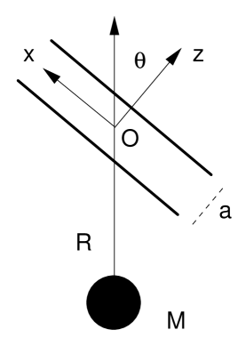
FIG. 1.: The orientation of the parallel conducting plates is shown. The origin of the coordinate system is marked by the letter O, and the mass M is located at $(-R\sin\theta,\,0,\,-R\cos\theta)$.

REFERENCES

- [1] H. Casimir, Proc. K. Ned. Akad. Wet. 51, 793 (1948).
- [2] H. Casimir and D. Polder, Phys. Rev. 73, 360 (1948).
- [3] S. Weinberg, Rev. Mod. Phys. 61, 1 (1989).
- [4] S. M. Carroll, Living Rev. Rel. 4, 1 (2001) [arXiv:astro-ph/0004075].
- [5] Ya. B. Zel’dovich, Soviet Physics Uspekhi 11, 381-393 (1968) [Usp. Fiz. Nauk 95, 209-230 (1968)].
- [6] For a review of dark energy experiments, and other efforts to measure the accelerating cosmic expansion, see the Dark Energy Resource Book at snap.lbl.gov/evlinder/sci.html.
- [7] G. Bressi, G. Carugno, R. Onofrio and G. Ruoso, Phys. Rev. Lett. 88, 041804 (2002) arXiv:quant-ph/0203002.
- [8] M. Bordag, U. Mohideen and V. M. Mostepanenko, Phys. Rept. 353, 1 (2001) [arXiv:quant-ph/0106045].
- [9] K. A. Milton, “The Casimir Effect: Physical Manifestations Of Zero-Point Energy,” River Edge, USA: World Scientific (2001).
- [10] M. Karim, A. H. Bokhari and B. J. Ahmedov, Class. Quant. Grav. 17, 2459 (2000).
- [11] J. Schwinger, L. L. DeRaad, Jr., K. A. Milton, W.-Y. Tsai, “Classical Electrodynamics,” Reading, Mass.: Perseus Books (1998).
- [12] D. Deutsch and P. Candelas, Phys. Rev. D 20, 3063 (1979).
- [13] G. Kennedy, R. Critchley and J. S. Dowker, Annals Phys. 125, 346 (1980).
- [14] L. S. Brown and G. J. Maclay, Phys. Rev. 184, 1272 (1969).
- [15] E. Calloni, L. Di Fiore, G. Esposito, L. Milano and L. Rosa, Phys. Lett. A 297, 328 (2002) [arXiv:quant-ph/0109091].
- [16] C. M. Will, “Theory and Experiment in Gravitational Physics,” (revised edition), Cambridge University Press (1993).
- [17] A. P. Lightman, W. H. Press, R. H. Price, S. A. Teukolsky, “Problem Book in Relativity and Gravitation,” Princeton, NJ: Princeton University Press (1975).
- [18] C. W. Misner and P. Putnam Phys. Rev. 116, 1045 (1959).
- [19] W. de Sitter, Mon. Not. Roy. Astron. Soc. 78, 3 (1917); reprinted in “Cosmological Constants,” eds. J. Bernstein and G. Feinberg, Columbia University Press: New York (1986).
- [20] A. Einstein, Akad. d. Wiss. 1917, 142 (1917); reprinted in “Cosmological Constants,” eds. J. Bernstein and G. Feinberg, Columbia University Press: New York (1986).
- [21] L. Parker, Phys. Rev. D 22 (1980) 1922.
- [22] M. T. Jaekel and S. Reynaud, J. Phys. I(France) 3, 1093 (1993).
- [23] L. Viola and R. Onofrio, Phys. Rev. D 55, 455 (1997) [arXiv:quant-ph/9612039].
- [24] M. T. Jaekel and S. Reynaud, Rept. Prog. Phys. 60, 863 (1997) [arXiv:quant-ph/9706035].
- [25] G. Papini, arXiv:gr-qc/0110056.