On biases in the predictions of stellar population synthesis models

Abstract

Sampling fluctuations in stellar populations give rise to dispersions in observables when a small number of sources contribute effectively to the observables. This is the case for a variety of linear functions of the spectral energy distribution (SED) in small stellar systems, such as galactic and extragalactic Hii regions, dwarf galaxies or stellar clusters. In this paper we show that sampling fluctuations also introduce systematic biases and multi-modality in non-linear functions of the SED, such as luminosity ratios, magnitudes and colours. In some cases, the distribution functions of rational and logarithmic quantities are bimodal, hence complicating considerably the interpretation of these quantities in terms of age or evolutionary stages. These biases can be only assessed by Monte Carlo simulations. We find that biases are usually negligible when the effective number of stars, $\cal{N}$, which contribute to a given observable is larger than 10. Bimodal distributions may appear when $\cal{N}$ is between 10 and 0.1. Predictions from any model of stellar population synthesis become extremely unreliable for small $\cal{N}$ values, providing an operational limit to the applicability of such models for the interpretation of integrated properties of stellar systems. In terms of stellar masses, assuming a Salpeter Initial Mass Function in the range 0.08 – 120 M_⊙, $\cal{N}$=10 corresponds to about 10⁵ M_⊙ (although the exact value depends on the age and the observable). This bias may account, at least in part, for claimed variations in the properties of the stellar initial mass function in small systems, and arises from the discrete nature of small stellar populations.

1 Introduction and motivation

The comparison of observations to theoretical models is one of the basic steps which allows an understanding of natural phenomena. The comparison is not always satisfactory and leads to either new insights on the nature of the phenomena observed or to revisions of the theoretical framework within which the models are made, or both.

In general models have an intrinsic uncertainty, in addition to possible systematic effects, and one seeks to minimise both in order to infer a robust interpretation of the observations. In the case of stellar population synthesis, the former uncertainties have often been neglected in comparison with the latter, where external errors (i.e. uncertainties on the input assumptions) have been much discussed, e.g. Leitherer et al. (1996) or Bruzual (2001). However, the predicted integrated properties of small stellar systems suffer from large intrinsic dispersions arising from the very nature of the systems: sampling fluctuations from, say, the initial mass function (IMF) will give rise to fluctuations in the properties and hence to an intrinsic dispersion in the predictions (e.g. Chiosi et al. 1988; Santos & Frogel 1997; Lançon & Mouhcine 2000; Cerviño et al. 2000, 2001; Bruzual 2002; Cerviño et al. 2002). This effect has been overlooked by most synthesis codes, which usually take an analytical IMF and produce predictions which are only valid in the limit where the number of stars is formally infinite.

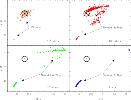
Figure 1: Integrated $B-V$ colour vs. $V-K$ colour of 10 Myr old stellar clusters with 1000, 100, 10 and 1 star, respectively, with masses between 2 and 120 M_⊙ distributed following a Salpeter IMF (triangles). Each triangle represents a Monte Carlo simulation with these parameters. The location of a stellar population with an infinite number of stars is indicated with the $\odot$ symbol. The colours of the sparsely-populated clusters show a multimodal distribution in this diagram, and their average values are biased with respect to the colours of an infinite stellar population.

In addition to this dispersion –which can be quantified and properly taken into account with the tools developed by Cerviño et al. (2002)– there is also a more subtle effect arising from this incomplete sampling. Integrated quantities which scale linearly with the number of stars (such as the luminosity in a given photometric band, or the overall spectral energy distribution, SED) can be predicted for any stellar system from the scaled-down outputs of synthesis codes with effectively predict properties for very large stellar systems, that is, systems which fully sample the distribution function of masses. However, for quantities which do not scale linearly with the number of stars, such as luminosity ratios, magnitudes, colours, equivalent widths, etc, such a scaling cannot be performed properly, and the only solution is to make extensive Monte Carlo simulations. We can already foresee that biases will arise from the incomplete sampling of the underlying distribution function. For instance, infrared colours may be dominated, at some ages, by a handful of high luminosity, IR-bright stars. Monte Carlo simulations calculated by Santos & Frogel (1997)  show that the average colour is a function of the number of stars in the simulation. Similarly, the average optical colours of stellar clusters, at a given age, are functions of the total mass in the cluster, as shown for instance by Girardi & Bica (1993) and more recently by Girardi (2000) and Bruzual (2002).

This is best illustrated with an example in a simple colour-colour diagram. Figure 1 shows the point (indicated by the $\odot$ symbol) where a 10 Myr-old stellar population with an infinite number of stars would be. Each triangle in each panel represents one Monte Carlo simulation of a 10 Myr-old stellar population with a total number of stars (with masses between 2 and 120 M_⊙ distributed with a Salpeter IMF) of 1000, 100, 10 and 1 star, respectively. Figure 1 shows three important effects:

(a) The distribution of colours in this diagram is clearly bimodal or even multimodal. The points do not cluster around a well-defined center, but are very scattered over the entire diagram, at odds with the (standard) predicted value for an infinitely-large stellar population.

(b) If the average colour is computed for clusters with the same number of stars, its value is very different from the one given by the standard prediction : the average colour is biased, and the bias depends on the total number of stars present in the population.

(c) The area covered by the points (each representing one Monte Carlo simulation) is not a monotonic function of the number of stars in the simulation.

Note that these effects are not limited of course to clusters of this age, but do also appear in more evolved populations, since these effects are a generic feature of under-sampled clusters.

In this paper we provide a first order analytical estimation on when and why synthesis models which use an analytical formulation of the IMF are not be able to reproduce the observed properties of stellar systems and therefore when Monte Carlo simulations are absolutely required in order to make predictions. We show that bias and multimodality features are a generic property of non-linear functions of the SED, and will always be present when trying to apply population synthesis models to small size stellar populations. Their importance cannot be stressed enough: many of the seemingly ’peculiar’ properties of some systems can, at least in part, be accounted for by this bias and multimodality effects.

This is an important issue since odd values of these properties often lead to non standard interpretations. For instance, when colours or equivalent widths (EWs) of small stellar systems appear to be peculiar (that is, peculiar with respect to the values predicted by synthesis models of a large number of stars), they are often interpreted in terms of IMF variability : either the mass cutoffs have to be truncated, and/or the slope of the IMF has to be changed in order to produce the ’correct’ colours or EWs. Since the lower mass cutoff determines the overall mass-to-light ratio, it is usually the upper mass limit which is varied to account for the data. Examples of these interpretations abound in the recent literature, starting perhaps with Shields & Tinsley (1976) who, on the basis of the variation of the equivalent width of H$\beta$ in Hii regions across M 101, inferred a dependence of the upper mass cutoff with metallicity. Line ratios included in classical diagnostic diagrams have also been used (e.g. Olofsson 1997, and Bresolin, Kennicutt & Garnett 1999 for the softness parameter) and seem to show that the IMF changes in extragalactic Hii regions (but see however Bresolin & Kennicutt 2002, for an alternative explanation based on sampling effects). Colours, and colour-colour diagrams, sometimes including the H$\alpha$ line, of clusters and starbursts also seem to point to variations in the parameters of the IMF, from the LMC (Dolphin & Hunter 1998), to clusters in the starburst galaxy IC10 (Hunter 2001).

The common features of all these interpretations which point to a variation of the IMF are (i) the systematic use of non-linear quantities (EWs, line ratios, colours) and (ii) observations of small stellar systems (Hii regions, stellar clusters, starbursts, etc).

Given the scaling arguments explained above, it is interesting to see whether sampling effects could account for this type of observations. In this paper we show that whilst the average values of the properties (and their dispersions) that scale with the number of stars are reasonably well reproduced by the models, non-linear functions such as luminosity ratios or colours may be heavily biased. It is beyond the scope of this paper to analyse in detail each and every observation, but given our results, it appears very likely that the ’peculiar’ properties observed in some systems can be simply understood in terms of the bias and multimodality introduced by sampling fluctuations of the IMF in these stellar systems. This has profound implications for the interpretation of colours, average magnitudes and line ratios in such systems, as well as for the universality (or otherwise) of the IMF. These effects seem to be large enough that most observations may point to the universality of the IMF, despite a variety of physical conditions (e.g. Kroupa 2002 for a general review and Mas-Hesse & Kunth 1999 for the case of starburst galaxies), and therefore provide a unique insight on star formation processes in a variety of environments.

The structure of the paper is the following: in Sec. §2 we recall the scaling properties of synthesis models. In Sec. §3 we analyse the statical properties of functions of the SED, showing the biases and multimodalities that appear in their distribution functions. We discuss these results and their implications in Sec. §4 and §5.

2 On sampling and scaling in population synthesis

Population synthesis models often scale predictions to the total mass in stars. There are at least two reasons for this. First, a (suitable) fixed mass-to-light ratio can be achieved. Second, the predictions, which are made for a unit star formation rate (that is, the rate at which a given gas mass is transformed into stars), can be scaled to other rates, or, equivalently, to other masses in gas or stars.

The underlying mathematical justification for this scaling is simple to see. Take for example the average total luminosity in a given band $\mu_{L}=<L>$. This is given by the weighted sum of the luminosities $L_{i}$ of the $N_{\mathrm{tot}}$ stars present in a population at some given age :

$$\mu_{L}(N_{\mathrm{tot}})\;=\;\sum_{i=1}^{I}\,n_{i}L_{i},$$ (1)

where $I$ is the number of initial (zero-age) masses considered such that $N_{\mathrm{tot}}=\sum_{i=1}^{I}\,n_{i}$ and $n_{i}$ is the (integer) number of stars of type or class $i$. For a sample of different size $N{{}^{\prime}}_{\mathrm{tot}}$, all other parameters kept the same (age, metallicity, etc), the following scaling applies:

$$\mu_{L}({N_{\mathrm{tot}}})\;/\;N_{\mathrm{tot}}\;\;=\;\;\mu_{L}({N{{}^{\prime}}_{\mathrm{tot}}})\;/\;N{{}^{\prime}}_{\mathrm{tot}}.$$ (2)

This scaling arises because, at a fixed age, $L_{i}$ are constants whilst $n_{i}$ follow a Poisson distribution (see Cerviño et al. 2002), and the average value of a (weighted) sum of Poisson variables is the (weighted) sum of average values. It is this linear scaling that allows predictions made for a given $N_{\mathrm{tot}}$ to be scaled up or down for a different number of stars.

However, the scaling is always made with the total mass in stars, not the actual number of stars $N_{\mathrm{tot}}$ present in a population. Obviously, for a fixed IMF, there is a direct relation between the total mass in stars and the number of stars, but there is an important difference in that the total mass, $M_{\mathrm{tot}}$ is a random variable when $N_{\mathrm{tot}}$ is fixed (and vice versa).

The PDF of $M_{\mathrm{tot}}$, as of any function of the IMF, can be obtained analytically using the characteristic function method (e.g. Kendall & Stuart 1977), although the inversion can be cumbersome or indeed unworkable. For the purposes of the present paper it is enough to show the PDF of $M_{\mathrm{tot}}$ obtained from Monte Carlo simulations.

Figure 2: Probability distribution function (PDF) of the total mass $M_{\mathrm{tot}}$ of clusters containing 1000, 100, 10 and 1 stars based on 10⁴ simulations ($5\times 10^{4}$ for the case of ’clusters’ with 1 star). The PDF in the case of only 1 star is trivially the IMF.

For $N_{\mathrm{tot}}=1$ the PDF of $M_{\mathrm{tot}}$ is trivially the IMF itself (see Fig. 2 bottom right), while for large values of $N_{\mathrm{tot}}$ the central limit theorem ensures that it converges to a Gaussian function (Fig. 2 top left). For intermediate values of $N_{\mathrm{tot}}$, the distribution has a heavy tail at large values of $M_{\mathrm{tot}}$, as Fig. 2 shows. Note also that this tail is not sampled well enough even though 10⁴ simulations were made, with clusters populated by 1000 stars of masses between 2 and 120 M_⊙ distributed with a Salpeter IMF. The heavy tails are a direct result of the poor sampling of the upper mass range, where the presence of a few massive stars can be very significant for the total mass in a small system.

The large dispersion in $M_{\mathrm{tot}}$, at $N_{\mathrm{tot}}$ fixed, shows that synthesis models which use an analytical ’sampling’ of the IMF overlook a fraction of the intrinsic dispersion inherent to the nature of the problem: small stellar systems will always show a dispersion in $M_{\mathrm{tot}}$ event though $N_{\mathrm{tot}}$ is kept fixed, and inversely. So not only using $N_{\mathrm{tot}}$ is the natural choice for the scaling, but it also leads to take into account one of the factors which produce an intrinsic dispersion in the observables.

The evaluation of the dispersion in $M_{\mathrm{tot}}$ requires to know the corresponding PDF, but we can estimate how it scales with $N_{\mathrm{tot}}$ from the results of the Monte Carlo simulations. Let us assume that the IMF, $\Phi(m)$, is given by a power law:

$$\frac{dN}{dm}=\Phi(m)=Am^{-\alpha},$$ (3)

where $A$ is a normalisation constant. If the IMF is defined between some mass cutoffs $m_{\mathrm{low}}$ and $m_{\mathrm{up}}$, the normalisation constant is given by:

$$A = \frac{(1-\alpha)}{m_{\mathrm{up}}^{1-\alpha}-m_{\mathrm{low}}^{1-\alpha}}.$$ (4)

In the case of only one star, the average value of the stellar mass is given by

$$<m> = \int_{m_{\mathrm{low}}}^{m_{\mathrm{up}}}m\,\Phi(m)\,dm=\;$$ (5)

$$= \frac{A}{(2-\alpha)}\,\left(m_{\mathrm{up}}^{2-\alpha}-m_{\mathrm{low}}^{2-\alpha}\right)$$

$$= \frac{(1-\alpha)\,(m_{\mathrm{up}}^{2-\alpha}-m_{\mathrm{low}}^{2-\alpha})}{(2-\alpha)\,(m_{\mathrm{up}}^{1-\alpha}-m_{\mathrm{low}}^{1-\alpha})},$$

and its variance by

$$\sigma^{2}(m) = \int_{m_{\mathrm{low}}}^{m_{\mathrm{up}}}(m-<m>)^{2}\,\Phi(m)\,dm$$ (6)

$$= \frac{(1-\alpha)(m_{\mathrm{up}}^{3-\alpha}-m_{\mathrm{low}}^{3-\alpha})}{(3-\alpha)(m_{\mathrm{up}}^{1-\alpha}-m_{\mathrm{low}}^{1-\alpha})}-<m>^{2}.$$

so, square of its relative error is

$$\frac{\sigma(m)^{2}}{<m>^{2}} = \left[\frac{(2-\alpha)^{2}\,(m_{\mathrm{up}}^{3-\alpha}-m_{\mathrm{low}}^{3-\alpha})}{(3-\alpha)(m_{\mathrm{up}}^{2-\alpha}-m_{\mathrm{low}}^{2-\alpha})^{2}}\right]\times$$ (7)

$$\left[\frac{(m_{\mathrm{up}}^{1-\alpha}-m_{\mathrm{low}}^{1-\alpha})}{(1-\alpha)}\right]-1.$$

For the particular case of a Salpeter IMF, with cutoffs at 2 and 120 $M_{\odot}$, these values are $<m>=5.897$, $\sigma(m)^{2}=76.28$ and $\sigma(m)/m$ = 1.481.

In general, $M_{\mathrm{tot}}$ is proportional to $N_{\mathrm{tot}}$. It can be seen that the variance, $\sigma(M_{\mathrm{tot}})^{2}$ is also proportional to $N_{\mathrm{tot}}$. Therefore the relative error in $M_{\mathrm{tot}}$ is inversely proportional to the square root of the number of stars.

For stellar populations with a large number of stars, the dispersion becomes negligible (e.g., 0.01 per cent for a system of 2$\times 10^{8}$ stars) and quantities which depend linearly on the number of stars can be normalised safely to $M_{\mathrm{tot}}$ rather than to $N_{\mathrm{tot}}$ (which becomes difficult to measure in such cases!).

3 Distribution functions and moments of observables in synthesis models

Figure 3: Temporal evolution of the average $L_{V}$ and $L_{K}$ luminosities and their corresponding effective number of stars, ${\cal N}$, normalised to the actual number of stars $N_{\mathrm{tot}}$. This is the evolution predicted for an infinite population of stars, fully sampling a Salpeter IMF between 2–120 M_⊙.

In order to establish how relevant the effect of sampling is, we have followed the evolution of each Monte Carlo simulation of stellar clusters of fixed $N_{\mathrm{tot}}$, and derived their integrated luminosities in the $V$ and $K$ bands.

Using the ensemble of simulations at fixed $N_{\mathrm{tot}}$, we have obtained mean values and dispersions for these luminosities, their $\log$, the $L_{V}/L_{K}$ ratio and the $V-K$ colour. To avoid introducing further parameters in this study, we used the Kurucz (1991) atmosphere models and solar metallicity tracks with standard mass-loss rates form Schaller et al. (1992). For the sake of simplicity, the nebular contribution to the luminosity has not been taken into account in these runs.

Although Monte Carlo simulations seem the natural, and only, way to estimate the PDF of any observable, Cerviño et al. (2002) showed that it is possible to apply a Poissonian formalism which allows the estimation of the first two moments of the PDF analytically. This formalism is based on the idea that there is only an effective number of stars, ${\cal N}$, which contribute to a given observable. Its definition is related to the quasi-Poissonian nature of the luminosity PDF. For example, for the observable monochromatic luminosity $L$, its effective number ${\cal N}(L)$ is given by the expression

$$\frac{1}{\sqrt{{\cal N}(\mathrm{L})}}=\frac{\sigma(\mathrm{L})}{\mu_{\mathrm{L}}},$$ (8)

as first derived by Buzzoni (1989).

Note that this effective number is not an actual number of stars, but rather a measure of the weighted number of sources which contribute to a given observable. The larger the effective number, the better determined will the observable be. Small values of ${\cal N}(L)$ indicate an intrinsically large dispersion, and typically arise when a few (real) stars dominate the observable. For instance in young clusters a few very massive stars may dominate the overall energy budget or the SED. In old stellar populations, a few Asymptotic Giant Branch stars (AGB) may change significantly the luminosity. Hence in both situations one expects an intrinsically large dispersion in the observable, a direct result of the discrete nature of these small populations which sample incompletely the IMF but dominate the observable.

Figure 3 shows, for reference, the time evolution of the $L_{V}$ and $L_{K}$ luminosities (normalised to the number of stars in the cluster), for a stellar population which fully samples the given IMF, that is, with an infinite number of stars in the indicated mass range, along with the evolution of their effective number of stars $\cal{N}$, which readily allows an estimate of the intrinsic dispersion in these luminosities via Eq. (8), for any stellar population of any size and any age. These were some of the results obtained by Cerviño et al. (2002).

It is interesting to see some values of $\cal N$. From Fig. 3 can be seen that $5(2.5)\times 10^{3}$ stars are needed to obtain ${\cal N}(L_{K})$ (${\cal N}(L_{V})$) values larger than 10. This means cluster masses around $3(1.5)\times 10^{4}$ M_⊙ in the mass range 2–120 M_⊙, and would the IMF be extended down to 0.08 M_⊙, the mass of the cluster would be $M_{\rm tot}$=$1.1(0.6)\times 10^{5}$ M_⊙.

For young stellar populations, ${\cal N}$ values for different luminosities normalised to the stellar cluster mass assuming a Salpeter IMF in the mass range 2-120 M_⊙ can be found in http://www.laeff.esa.es/users/mcs/SED/.

In the case of old stellar populations ${\cal N}$ has been computed directly by Buzzoni (1989). Additional estimations can be obtained from the evaluation of brightness fluctuations, $\bar{L}$ as shown by Buzzoni (1993).

3.1 Linear functions

Figure 4: Comparison between Monte Carlo simulations (Mon) and fully-sampled (Ana) of the average values and dispersions of $L_{V}$ (left) and $L_{V}$ (middle). The lines correspond to different sizes of stellar populations ($N_{\mathrm{tot}}$=1000 stars: solid, $N_{\mathrm{tot}}$=100 stars: dashed, $N_{\mathrm{tot}}$=10 stars: dot-dashed and $N_{\mathrm{tot}}$=1 star: dotted). The top panel on the right side give the correlation coefficient between both quantities (upper panel) by the simulations (lines) and the estimation proposed by Cerviño et al. (2002) (stars). The ratio between the Monte Carlo and fully-sampled estimates are shown ion the lower panels.

Figure 5: PDF distributions ${\cal G}(x)$ for $x=L_{V}/\mu(L_{V})$ at selected ages for a variety of sizes of stellar populations. Note that $\cal{N}$ is given only for clusters with $N_{\mathrm{tot}}$=1000 stars, since it scales linearly with $N_{\mathrm{tot}}$, that is, ${\cal{N}}(N_{\mathrm{tot}})={\cal{N}}(10^{3})\times(N_{\mathrm{tot}}/10^{3})$ for the other populations.

Figure 6: Same as Fig. 5 for $x=L_{K}/\mu(L_{K})$.

In general, a linear combination of Poisson variables will not be another Poisson variable, unless the weights take integer values (see Cerviño et al. 2002, for a discussion). However, the fact that it is a linear combination of random variables allows one to estimate exactly its first two moments, even though the remaining moments can sometimes be also determined analytically. This is well illustrated by Fig. 4 which shows the comparison of the Monte Carlo simulations with the fully-sampled results for the $L_{V}$ and $L_{K}$ observables. The agreement is very good in all cases, with small deviations when the number of stars in the cluster decreases. Except in rare occasions, the analytical expressions obtained via Eq. (8) are within 3 per cent and 5 per cent of the Monte Carlo ones. Not only the average values agree at this level (and hence are not biased) but also the estimation of the dispersion is very good, over a dynamical range of three orders of magnitude in the total number of stars. Linear functions of the luminosity (such as luminosities integrated in a photometric band, or ionising fluxes) are not biased.

Remarkably, our Poissonian formalism is also able to predict the mean value and dispersion for simulations of clusters which contain only one star. In this case, the IMF gives us the relative weight of the probability $w_{i}$ to obtain a star with a given luminosity $l_{i}$. The mean value, taking each cluster as a one realisation, is

$$\mu_{L}=\sum_{i=1}^{N_{sim}}\;l_{i}\,w_{i},$$ (9)

with dispersion

$$\sigma^{2}(L)=\sum^{N_{sim}}(l_{i}-\mu_{L})^{2}w_{i}=\sum^{N_{sim}}l_{i}^{2}w_{i}-\mu_{L}^{2}.$$ (10)

Eq. (8) implies that when ${\cal N}$ is very small $\sum l_{i}^{2}w_{i}>>\mu_{L}^{2}$, and so Poisson dispersions and Monte Carlo ones become very similar.

The highly variable correlation coefficient between $L_{V}$ and $L_{K}$ is also predicted correctly by the Poisson formalism, as shown on Fig. 4. The agreement is in fact at the 2 per cent level for most ages. It shows that a (variable) fraction of stars contribute in luminosity to both bands, and therefore the actual dispersions in these luminosities must take into account this important term if errors are to be evaluated properly. As Cerviño et al. (2002) showed, the effect of not including this term is to systematically underestimate the dispersion.

So far so good for the first two moments, but what about the actual shape of the PDF of these luminosities? Could the deviations from the Poisson formalism be accounted for deviations in the PDF? Figures 5 and 6 give these PDFs at selected ages in terms of the variable $x=L/<L>=L/\mu_{L}$. Note the logarithmic scale on the vertical axis. The vertical dashed lines give the values of $x=\mu^{\mathrm{Analytical}}_{L}/\mu^{\mathrm{MonteCarlo}}_{L}$, which, as shown above, are very close to unity and hence are not biased. It is interesting to note that whereas the mean value of the simulations are well reproduced, the median value and the most probable (mode) values are shifted to the left in all cases. This effect must be taken into account when the result of standard synthesis models are compared with individual clusters.

At early ages most stars are close to the ZAMS, and hence the mass-luminosity relation makes that the PDF in luminosity is very similar to the PDF distribution in total mass (compare with Fig. 2). As stars evolve, post-MS evolutionary stages are reached, and obviously the longer the stage, the better sampled it is. This gives rise to secondary peaks in the PDF, where stars can accumulate, leading to multi-modality in the luminosity distribution. The number of such stars will be smaller than 1 per cent of the stellar population of the cluster. When the total number of stars is low, there is a non-zero probability that the cluster will have no post-MS. So, for a given fixed number of stars, it is possible to have clusters (sharing the same total number of stars) with or without post-MS stars, a clear case of possible bimodality when the observable depends on the presence (or otherwise) of post-MS stars. This effect was first pointed out in the pioneering work by Chiosi et al. (1988). We stress again that the average values are not biased, and that the deviations from the Poisson distribution are relatively small in terms of the first two moments only. Obviously higher moments are far more sensitive to shorter evolutionary stages, and hence more prone to sampling effects.

We can nevertheless quantify these deviations in terms of $\cal{N}$. A Poisson distribution defined by a parameter smaller than ${\cal{N}}=5$, has a probability larger than 1 per cent to have a number of effective sources equal to zero. As mentioned before, the number of effective sources is not an actual number of stars, but rather a measure of the effect of (under-)sampling in these clusters. For $\cal{N}$ values between 5 and 0.1, the probability of having a cluster with zero effective sources increases from 1 per cent to 90 per cent. For even smaller values of $\cal{N}$ most clusters will have no effective sources in that band, because they do not contain stars in the suitable evolutionary phase which contributes to the observable. We therefore expect that when $\cal{N}$ is in the range between about 5 and 0.1 bimodality will be most easily observed.

Again, $\cal{N}$ is an observable-dependent quantity, so it is possible that some clusters have large $\cal{N}$ values for some quantities but small values for others. If these quantities are linear functions of the SED or the luminosity, then their average values are not biased. Any non-linear function will, on the contrary, be prone to biases and may enhance multimodality, as we show in the following sections.

3.2 Logarithmic functions

Figure 7: Comparison of average values and dispersions of $\log L_{V}$ and $\log L_{K}$ from Monte Carlo simulations and from Eqs. (11) and (12) (used in synthesis models with an infinite number of stars). The line styles and symbols correspond to different sizes of stellar populations ($N_{\mathrm{tot}}$=10³ stars : solid lines and circles, $N_{\mathrm{tot}}$=10² stars : dashed lines and squares, $N_{\mathrm{tot}}$=10 stars : dot-dashed lines and triangles and $N_{\mathrm{tot}}$=1 star : dotted). Symbols correspond to the use of Eq. (18). Filled symbols correspond to ${\cal N}(L)$ values lower than 1.

Figure 8: PDF of $\log L_{V}$ at selected ages. The vertical dashed line gives the position of $\log<L_{V}>$ and hence of the bias. Note the variable amount of bias as a function both of age and size of the stellar population.

Figure 9: PDF of $\log L_{K}$ at selected ages. The vertical dashed line gives the position of $\log<L_{K}>$ and hence of the bias. Note the variable amount of bias as a function both of age and size of the stellar population.

In general, standard synthesis codes compute logarithmic quantities assuming implicitely that their average value is the logarithm of the average. For the logarithm of the luminosity this would be for instance

$$\mu_{\log L}=<\log L>$$ (11)

and the corresponding dispersion would be evaluated as

$$\sigma^{2}(\log L)=(\log{\mathrm{e}})^{2}\frac{\sigma_{L}^{2}}{\mu_{L}^{2}}=\frac{(\log{\mathrm{e}})^{2}}{{\cal N}(L)}.$$ (12)

This is obviously not correct in general, since the assumption relies implicitely on an infinitely narrow-peaked PDF for $L$, which is seldom the case.

Let us assume a sample of observations of a definite-positive random variable $L$ described by a PDF ${\cal P}(L)$. The expectation value $\mu_{C}$ of any function of this variable $C=C(L)$ is

$$\mu_{C}\;=\;<C>\;=\;\int_{0}^{\infty}\,C(L)\,{\cal P}(L)\,dL.$$ (13)

Take for instance the case where $L$ is the luminosity in some photometric band. The corresponding magnitude is $M=a+b\ln L$, with $a$ some zero point and $b=-2.5\log_{10}\mathrm{e}$. Its average value is

$$\mu_{M}=\;<M> = \int_{0}^{\infty}M\,{\cal P}(L)\,dL$$ (14)

$$= a\,+\,b\,\int_{0}^{\infty}(\ln L)\,{\cal P}(L)\,dL.$$

With the new variable $x=L/\mu_{L}$, whose PDF is ${\cal G}(x)$ such that of course $\int{\cal G}(x)dx=\int{\cal P}(L)dL=1$, this results in

$$\mu_{M} = a\,+\,b\,\ln\mu_{L}\,+\,b\,\int_{0}^{\infty}(\ln x)\,{\cal G}(x)\,dx.$$ (15)

Therefore, unless ${\cal G}(x)=\delta(x-1)$ (where $\delta(x)$ is Dirac’s Delta function) –that is, when the PDF of $L$ is defined only at $\mu_{L}$ – the average of the logarithmic quantity will not be the logarithm of the average value of the variable. The proper computation of the ${\cal G}(x)$ functions can be only performed with a massive number of Monte Carlo simulations. From this properly-sampled ${\cal G}(x)$ one could extract samples of $x$ for any sample of size $N_{\mathrm{tot}}$, but this is obviously unpractical. If this is nevertheless not done, then the estimated values are very likely to be biased.

A rough estimate of the bias can be evaluated by expanding in Taylor series. For the magnitude $M$ this is

$$M=a+b\ln\mu_{L}+b\left(\frac{L-\mu_{L}}{\mu_{L}}-\frac{(L-\mu_{L})^{2}}{2}\frac{1}{\mu^{2}_{L}}+\cdots\right),$$ (16)

so that, to first order, the mean value of the magnitude, and its variance are

$$\mu_{M} = a\,+\,b\,\ln\mu_{L}\,-\,b\,\frac{\sigma^{2}_{L}}{2\mu^{2}_{L}}+...$$ (17)

$$= a\,+\,b\,\ln\mu_{L}\,-\,\frac{b}{2{{\cal N}}(L)}+...$$

$$\sigma^{2}_{M} = \frac{b^{2}\sigma^{2}_{L}}{\mu^{2}_{L}}\left(1-\frac{1}{4}\frac{\sigma^{2}_{L}}{\mu^{2}_{L}}+...\right)$$ (18)

$$= \frac{b^{2}}{{\cal N}(L)}-\left(\frac{b}{2{\cal N}(L)}\right)^{2}+...$$

To first order, the bias is then $\frac{b}{2{\cal{N}}(L)}$, so if ${\cal{N}}(L)$ is large enough, Eqs. (11) and (12) are good approximations. In many cases ${\cal{N}}(L)$ will be small and the bias important. Eq. (18) gives a lower limit to the bias (since higher order corrections were not taken into account) and the only way to estimate the bias is, inevitably, via Monte Carlo simulations. This is done in Fig. 7 where this analytical estimate is compared with the Monte Carlo ones (middle and right panels).

Alternatively, in terms of difference in magnitude

$${\Delta M_{L}}=\mu(M_{L})-M_{L}=2.5(\log L-\mu_{\log L}),$$ (19)

we see that the bias can reach some 0.5 magnitudes in $M_{V}$ and 2.5 magnitudes in $M_{K}$ for clusters with 100 stars between 2 and 120 $M_{\odot}$, and 2 magnitudes in $M_{V}$ and $\sim 5$ magnitudes in $M_{K}$ for groups of 10 stars in that mass range. We can also see that using Eqs. (11) and 12 give systematically wrong results, because they predict systematically too large values. This is easy to understand since they assumed a fully-sampled IMF, were massive stars are (comparatively) over represented with respect to Monte Carlo samples of small size. The estimates given by Eq. (18) are indicated with symbols in Fig. 7. Although they fail to give the correct correction (due to the lack of higher order terms) in the bias, they provide a rough indication of the underestimation in the dispersion.

Figs. 8 and 9 present the PDFs of $\log L_{V}$ and $\log L_{K}$ respectively. In clusters with ${\cal{N}}(L_{V})$ or ${\cal N}(L_{K})$ larger than 10 (see Figs. 5 and 6), the PDFs are unimodal, as expected. However, for smaller values of ${\cal{N}}$ the situation is entirely different. In this case, the cluster is dominated by main sequence stars, which do not sample properly the IMF, given their small numbers, and in particular the upper mass end.

At 5.5 and 10 Myr, the $L_{V}$ distribution of clusters with 100 stars have ${\cal{N}}(L_{V})$ values of 0.7 and 2.5 respectively (see Fig. 5). The associated PDFs of $\log L_{V}$ show a bimodal structure with two peaks of similar amplitude (Fig. 8). The effect is more extreme in the case of $\log L_{K}$ (Fig. 9) were bimodality is present even for clusters with 1000 stars (in the 2–120 $M_{\odot}$ mass range) at 5.5 Myr with ${\cal{N}}(L_{K})=2.3$ (see also the PDFs at 5.5 and 10 Myr for clusters with 100 stars, with ${\cal{N}}(L_{K})$ values of 0.23 and 0.54 respectively). Bimodality with peaks of roughly similar amplitude implies that real clusters should have (log)luminosities peaking around (roughly) two values (barring selection effects, etc). One could naively think that these are two distinct populations of clusters where in fact there is only one. Since the total number of stars is the same, one could be driven to conclude, mistakenly, that the IMF in these two ’populations’ is different, while in fact it is just a sampling effect.

A final comment on simulations of clusters with one star, because their PDFs help to understand the origin of multimodality and bias. At 0.5 Myr the PDF is roughly a power law (the convolution of a IMF power law with the power-law relation between mass and luminosity for main sequence stars). Figs. 8 and 9 indeed show a linear relation in these log-log plots. As time goes by, the more luminous stars (i.e. the most massive ones) leave the main sequence, and become more luminous than the brighter main sequence stars. The PDFs show two distinct régimes: (i) a power-law for the less massive (and thus dimmer) stars, and (ii) secondary peaks for the longer post-MS evolutionary phases. When more massive clusters are considered, these post-MS peaks grow in importance, become better sampled, and eventually the bias disappears.

3.3 Rational and log-rational functions

Figure 10: Mean values and dispersions of $L_{V}/L_{K}$ in Monte Carlo simulations and in fully-sampled synthesis (via Eqs. (20) and (21), as used in standard synthesis models). Symbols and lines as in Fig. 7 except for filled symbols, that now correspond to ${\cal N}(L_{V})$ and ${\cal N}(L_{K})$ values lower than 10. Note that the $\sigma$ value for clusters with $10^{3}$ stars is larger at 5 Myr than the $\sigma$ value for ’clusters’ with one star. It is due to the PDF (Fig. 11) of the clusters with one star, see text for explanations.

Figure 11: PDF at selected ages of the $L_{V}/L_{K}$ ratio. The standard (naive) theoretical values are shown with vertical dashed lines.

Rational functions of luminosities are even more important in the interpretation of the properties of small stellar systems because, naively, they seem to be independent of normalisation problems, since the usual scaling with mass or number of stars cancels out. But this may not be necessarily the case, and, in addition, their dispersion due to the uneven sampling of the IMF can be dramatically large.

In standard synthesis models it is assumed that for a rational function $u=x/y$ its average value is given by

$$\mu_{u}\;=\;\mu_{x}\times\mu_{1/y}\;=\;\mu_{x}/\mu_{y},$$ (20)

and its dispersion is given by:

$$\frac{\sigma_{u}^{2}}{\mu^{2}_{u}} \simeq \frac{\sigma_{x}^{2}}{\mu^{2}_{x}}+\frac{\sigma_{y}^{2}}{\mu^{2}_{y}}-2\frac{{\mathrm{cov}}(x,y)}{\mu_{x}\,\mu_{y}}$$ (21)

$$= \frac{1}{{\cal N}(x)}+\frac{1}{{\cal N}(y)}-2\frac{\rho(x,y)}{\sqrt{{\cal N}(x)\,{\cal N}(y)}}=\frac{1}{{\cal N}(u)},$$

where $\rho(x,y)=\frac{\mathrm{cov}(x,y)}{\sigma_{x}\,\sigma_{y}}$ is the correlation coefficient between $x$ and $y$.

Again, this would be correct if the distribution of $u$ would be a very narrow peak, but in the general case this is not correct. For a function $R=1/L$, the average value is given by

$$\mu_{R}\;=\;\int_{0}^{\infty}\,\frac{1}{L}{\cal P}(L)\,dL=\;\frac{1}{\mu_{L}}\int_{0}^{\infty}\frac{1}{x}\,{\cal G}(x)\,dx,$$ (22)

where $x=L\,/\mu_{L}$. Again, unless ${\cal G}(x)=\delta(x-1)$,

$$\mu_{R}\;=\;\mu_{1/L}\;\neq\;1/\mu_{L},$$ (23)

and, more generally,

$$\mu(L_{1}/L_{2})\;\neq\;\mu_{L_{1}}/\mu_{L_{2}}.$$ (24)

With a second-order Taylor expansion one gets, to first order

$$\mu_{R} = \frac{1}{\mu_{L}}\left(1+\frac{\sigma^{2}_{L}}{\mu^{2}_{L}}+...\right)=\frac{1}{\mu_{L}}\left(1+\frac{1}{{\cal{N}}(L)}+...\right)$$

$$\sigma^{2}_{R} = \frac{\sigma^{2}_{L}}{\mu^{4}_{L}}\left(1-\frac{\sigma^{2}_{L}}{\mu^{2}_{L}}+...\right)$$

$$= \frac{1}{\mu^{2}_{L}\,{\cal{N}}(L)}\left(1-\frac{1}{{\cal{N}}(L)}+...\right),$$

and, in general, for a rational function $u=x/y$

$$\mu_{u} = \frac{\mu_{x}}{\mu_{y}}\left(1+\frac{\sigma^{2}_{y}}{\mu^{2}_{y}}\right)-\frac{\mathrm{cov}(x,y)}{\mu^{2}_{y}}+...$$

$$= \frac{\mu_{x}}{\mu_{y}}\left(1+\frac{1}{{\cal{N}}(y)}-\frac{\rho(x,y)}{\sqrt{{\cal N}(x)\,{\cal N}(y)}}\right)+...$$

$$\sigma^{2}_{u} = \frac{\sigma^{2}_{x}}{\mu^{2}_{y}}+\frac{\mu^{2}_{x}\,\sigma^{2}_{y}}{\mu^{4}_{y}}-\frac{2\,\mu_{x}\mathrm{cov}(x,y)}{\mu^{3}_{y}}-$$

$$\left(\frac{\mu_{x}\,\sigma^{2}_{y}}{\mu^{3}_{y}}-\frac{\mathrm{cov}(x,y)}{\mu^{2}_{y}}\right)^{2}+...$$

$$\frac{\sigma_{u}^{2}}{u^{2}} = \frac{1}{{\cal N}(x)}+\frac{1}{{\cal N}(y)}-2\frac{\rho(x,y)}{\sqrt{{\cal N}(x)\,{\cal N}(y)}}-$$ (26)

$$\left(\frac{1}{{\cal N}(y)}-\frac{\rho(x,y)}{\sqrt{{\cal N}(x)\,{\cal N}(y)}}\right)^{2}+...$$

To first order approximation, the bias is then of the order of $\frac{\mu_{x}}{\mu_{y}}\left(\frac{1}{{\cal N}(y)}-\frac{\rho(x,y)}{\sqrt{{\cal N}(x)\,{\cal N}(y)}}\right)$, and the correct estimation of the mean value of a ratio requires the covariance between the numerator and denominator.

Again, we illustrate here these effects with the simple ratio $L_{V}/L_{K}$ in Fig. 10, where Eqs. (20) and (21) produce a very severe bias, even larger than one order of magnitude, both in the average and in the dispersion. The symbols show the results using Eq. (26) and they have the same meaning as in Fig. 7 except for filled symbols, which now correspond to ${\cal N}(L_{V})$ and ${\cal N}(L_{K})$ values lower than 10. In this case, the use of the Eq. (26) only produces a marginally better result than Eq. (20). Note that in the case of $\sigma(L_{V}/L_{K})$ there are fewer points computed with Eq. (26) than in the case of the mean value. This is just because, for some values, Eq. (26) produces negative $\sigma^{2}(L_{V}/L_{K})$ values and the use of these equations is not valid. It is interesting to see that the bias can be positive or negative, a direct consequence of the time variability of the correlation coefficient between the two luminosities.

The corresponding PDFs are given in Fig. 11. In this case, bimodality is apparent for a wide range of situations, and again, it is due to a secondary peak with larger values of the $L_{V}/L_{K}$ ratio. The bias may increase or decrease the average value, as shown by the vertical dashed lines. It is remarkable to see that the actual dispersion for the more massive clusters, at 10 Myr for example, is actually larger than the dispersion in less massive clusters. Again this is due to the presence of very massive stars, better sampled in these massive clusters, which have in comparison a much smaller flux in the $K$ band, and hence a very large $L_{V}/L_{K}$ ratio. The behaviour of the bias with the number of stars is clearly non-monotonic, as shown also in Fig. 10.

Finally, in the case of log-rational functions (such as integrated colours) there will be a priori a double bias, arising from the use of two non-linear functions. And yet most codes will still assume that the colours of a stellar population will not depend on its total mass. We take again as an example the $V-K$ colour. To first order,

$$\mu_{V-K} = a\,+\,b\,\ln\frac{\mu_{L_{V}}}{\mu_{L_{K}}}$$

$$-\,\frac{b}{2}\left(\frac{1}{{\cal N}(L_{V})}-\frac{1}{{\cal N}(L_{K})}\right)+...$$

$$\sigma^{2}_{V-K} = b^{2}\left(\frac{1}{{\cal N}(L_{V})}+\frac{1}{{\cal N}(L_{K})}-2\frac{\rho(x,y)}{\sqrt{{\cal N}(L_{V})\,{\cal N}(L_{K})}}\right)-$$ (27)

$$\,\frac{b^{2}}{4}\left(\frac{1}{{\cal N}(L_{V})}-\frac{1}{{\cal N}(L_{K})}\right)^{2}+...$$

Note that in this case the bias does not dependent on the correlation coefficient, and it has a value of approximately $\frac{b}{2}\left(\frac{1}{{\cal N}(L_{V})}-\frac{1}{{\cal N}(L_{K})}\right)$. Since redder wavelengths have a lower $\cal{N}$ value (in this range of ages) than shorter wavelengths (see Cerviño et al. 2002, for details), this approximation for the bias indicates that predictions of synthesis models must be corrected with a blue shift in order to get back to the actual mean value of a set of observed clusters. Note that for older clusters (say, above 1 Gyr or so), the trend is reversed since redder wavelengths (cooler evolutionary phases) become better sampled.

The situation is illustrated in Figs. 12 and 13. The top right panel of Fig. 12 shows the mean $V-K$ colour for the different sets of simulations. In this case, the difference between actual colours and those predicted by fully-sampled synthesis models can reach more than 3 magnitudes, even for the most massive clusters.

Figure 12: Mean values and dispersions of the integrated $V-K$ colour, from Monte Carlo simulations, and their comparison to simulation results obtained directly from the corresponding band luminosities. Symbols as in Fig. 10.

Figure 13: PDFs at selected ages for the $V-K$ colour. Naive theoretical values are shown with short-dashed vertical lines.

In the case of young star forming regions (younger than some 20 Myr), red colours have lower $\cal{N}$ values than blue ones (see Cerviño et al. 2002, for details). The resulting bias shows that the predictions of synthesis models must be corrected toward blue colours in order to reproduce the mean value of a set of observed clusters. At older ages, the bias may turn to bluer or redder values depending on the age, that is, on the proportion of post-MS versus main sequence stars.

Another interesting result shown in Figs. 10 and 12 is the corresponding $\sigma$ value. In the case of Gaussian distributions, $\sigma$ corresponds to the half width of maximum at about 60 per cent of the full height. In our case, the PDFs are not Gaussians, but $\sigma$ still gives us the width of the distribution at some (undefined) height. The Monte Carlo simulations show that at some ages (when post-MS stars appear in the clusters), the $\sigma$ value is maximum for the simulations with 100 stars and decreases for even fewer stars. This value is also related with the area covered by the simulations in Fig. 1, where the ’dispersion’ in the diagram is maximum for simulations with 100 stars. As we have already seen, this maximum $\sigma$ value is also related with a larger probability of obtaining bimodal distributions. The reason of this behaviour is that most of the clusters with a smaller number of stars will not have the post-MS phases sampled at all. This is also consistent with the lack of evolution in the $L_{V}/L_{K}$ ratio and the $V-K$ colour. So, the probability of finding a cluster with post-MS falls below the width of the level defined by $\sigma$. For more populated clusters, almost all of them will be reproduced correctly by standard synthesis models with a non-zero number of post-MS stars.

It is worth emphasizing that this behaviour is also present in simulations performed by Bruzual (2002). In his diagrams there is a maximum dispersion for the simulations with 10⁴ $M_{\odot}$ that decreases for simulations with 10³ $M_{\odot}$. Also, the bias effect is clearly present in his Monte Carlo simulations since the colours of these simulations do not agree with his analytical predictions.

4 Discussion and implications

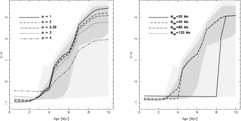
Figure 14: Evolution of the $V-K$ colour for different IMF slopes (left, assuming that $M_{\mathrm{up}}$= 120 M_⊙) and M_up values (right, assuming a Salpeter IMF slope). The areas in dark gray shade corresponds to the 90 per cent confidence interval for clusters with 1000 stars. The areas in light gray shade corresponds to the maximum and minimum values obtained in simulations of clusters with 1000 stars.

The comparison of observations with the results of a population synthesis method is in fact an inverse problem : Given the data, what are the models which best fit the data, given the errors in the data? It is seldom the case that errors within the models are also taken into account. It is also important to analyse whether the best fitting models are also good fits, and whether the solution is unique or not. In the case of synthesis models this procedure is often neglected and a variation in the input parameters is much preferred.

We have shown in the previous sections two major problems. First, the usual scaling with the total mass of the stellar population should not be made when dealing with small systems (dwarf galaxies, starbursts, stellar clusters, pixels, etc). Second, observables which are non-linear functions of the SED (or equivalently of the monochromatic luminosity) may present not only multimodal distribution functions, but also a systematic bias in the average values of these observables, with respect to the values predicted by codes which fully sample the IMF.

These effects have been overlooked in the past, because most synthesis codes do not provide an estimate of the intrinsic dispersion of the observables. Whilst this was easy to understand when dealing with the integrated properties of massive stellar populations, such as spiral and elliptical galaxies, this becomes a serious problem if such codes are applied to smaller stellar systems. Formally, the first moment of the PDF of a given observable cannot be scaled down properly. A possible solution would be to have the PDF of the observable and then extract samples of small size from that PDF. In this way the statistical properties of the observable, in small samples, can be analysed and compared with the observations.

The only proper solution to deal with the two problems we have discussed in this paper, multimodality and bias, is therefore to perform Monte Carlo simulations to construct the PDF of the observable. This is often unpractical, and we have shown that the quasi-Poisson formalism that we have developed can account for the statistical properties of the first two moments at a very good approximation level. Although the formalism cannot account for higher order moments, and thus to allow for strong deviations in the PDFs, it does not suffer from systematics and can easily (and should) be included in any synthesis code.

As we mentioned before, it has often been the case that the easiest solution to account for ’peculiar’ observations was to change some of the input parameters of the synthesis code, and in particular the properties of the IMF. It is well beyond the scope of this paper to analyse in detail each and every claim for variations of the IMF in small stellar systems, but we will illustrate here how sampling effects may have been mistakenly overlooked. We take again the $V-K$ colour, a non-linear function of the SED, as an example. Figure 14 (right panel) shows its evolution with time when the upper mass limit of the IMF is changed. It is readily apparent that if an observation gives a very blue $V-K$ colour, and all other parameters are the same (such as mass, luminosity, etc) within a small range, then it is tempting to hastily conclude that the upper mass limit in that particular system has to decrease. But in fact, as Fig. 12 shows, not only the average colour changes with the mass of the system, but also a large dispersion is expected, arising only from sampling fluctuations. Similarly, Fig. 14 (left panel) shows the effect of varying the slope of the IMF. Again, a too blue colour may be interpreted as evidence for a steeper slope. While our results cannot confirm or reject possible IMF variations in these systems, they however clearly indicate that part (if not all) of the dispersion in the $V-K$ colour may be accounted for by the incomplete sampling of a single, universal IMF.

Two final comments. First, in some cases there is no need for a bias to be present to explain some peculiar properties of small stellar systems. All the values quoted in Fig. 14 lie in fact in the predicted band quoted by the maximum and minimum $V-K$ values obtained from the simulations of clusters with 1000 stars (where the bias is small). The very large dispersion, an expected intrinsic property due to incomplete sampling, may account for many of the observed values, with no need to invoke special properties. As an example, in high-metallicity regions with Wolf-Rayet stars, the dispersion of synthesis models around their mean value is enough to explain the observations, as shown by Bresolin & Kennicutt (2002).

Second, another interesting effect concerns the ages of these systems, as inferred from non-linear functions of the luminosity. Because these observables may have a wide, multimodal distribution function, the intrinsic dispersion which may be observed in a given sample is not necessarily a reflection of a variation in the properties of individual members of that sample. It appears very dangerous to infer ages or mass variations from these small systems.

5 Conclusions

In this work we have found important effects which have been overlooked in the application of population synthesis codes to small stellar systems such as clusters, starbursts, dwarf galaxies or pixels. Most current synthesis codes predict the average values of observables for an infinitely large population of stars, which samples perfectly a given IMF. Extrapolating these predictions to small stellar systems may be misleading.

First, scaling observables with the mass in stars is not correct for small systems. The proper scaling should be performed with the total number of stars present in the system.

Second, the distribution functions of observables which are non-linear functions of the monochromatic luminosity (or SED) may show multimodality. This implies that for a given population, of fixed size, and all other parameters kept the same, there will be a large dispersion in the observable, whose average value will not necessarily be the same as the one predicted when the IMF is fully sampled. Most synthesis codes will therefore lead to biased predictions when applied to small stellar systems.

Third, we have also shown that bimodality is a natural effect that appears when stellar systems are affected by sampling (i.e. the number of stars in the clusters is not enough to sample completely the IMF). It is related to the evolutionary speed of different masses, or in more graphical terms, to the absence/presence of stars in some evolutionary phases. This effect was already shown 14 years ago by Chiosi et al. (1988). We have now established the range of $\cal{N}$ values (from $\approx$ 5 to 1) where bimodality appears. An additional result is that bimodality will be more easily observed when infrared colours are used since such colours are more affected by the presence of short-lived post-MS phases.

Fourth, while we cannot confirm or reject the hypothesis of possible variations in the properties of the IMF in small stellar systems, these results suggest that an important fraction of the dispersion observed in non-linear observables is not necessarily evidence for IMF variations, but can rather be accounted for by sampling fluctuations.

Finally, we have also derived an operational limit to the validity of standard synthesis codes. There is a critical effective number of stars (unrelated to an actual number of stars), with a value of around 10, which defines a boundary where multimodality may appear, i.e. cluster masses larger than 10⁵ M_⊙ for a Salpeter IMF in the range 0.08 – 120 M_⊙ (but the exact value for the cluster masses depends on the age and the observable). Below this critical value, the results of the codes must be taken with caution, since not only they can be biased, but also they may underestimate the actual dispersion of the observable, and Monte Carlo simulations are required. The reason for the existence of this critical value is directly related to the presence (or otherwise) of stellar evolutionary stages which are not fully sampled in small systems.

We encourage the inclusion of the calculation of this effective number of sources for a given observable in all synthesis codes, so that observers (and theoreticians alike) can estimate the expected dispersion (and possible biases) in observables.

References

- Bresolin, Kennicutt & Garnett (1999) Bresolin, F., Kennicutt, R.C. & Garnett, D.R., 1999, ApJ 510, 104
- Bresolin & Kennicutt (2002) Bresolin, F. & Kennicutt, R.C., 2002, ApJ 572, 838
- Bruzual (2001) Bruzual, G. 2001, ApSSS 277, 221
- Bruzual (2002) Bruzual, G. 2002, in IAU Symp. 207, Extragalactic star clusters, eds. D. Geisler, E. Grebel and D. Minniti (San Francisco: Astr. Soc. Pacific), in press (astro-ph/0110245)
- Buzzoni (1989) Buzzoni, A. 1989, ApJS 71, 871
- Buzzoni (1993) Buzzoni, A. 1993, A&A 275, 433
- Cerviño & Mas-Hesse (1994) Cerviño, M. & Mas-Hesse, J.M. 1994, A&A 284, 749
- Cerviño et al. (2000) Cerviño, M., Luridiana, V., and Castander, F., 2000, A&A Letters 360, L5
- Cerviño et al. (2001) Cerviño, M., Gómez-Flechoso, M.A, Castander, F.J. et al. 2001, A&A 376, 422
- Cerviño et al. (2002) Cerviño, M., Valls-Gabaud, D., Luridiana, V. & Mas-Hesse, J.M. 2002, A&A 381, 51
- Chiosi et al. (1988) Chiosi, C., Bertelli, G. & Bressan, A. 1988, A&A 196, 84
- Dolphin & Hunter (1998) Dolphin, A. & Hunter, D. 1998, AJ 116, 1275
- Girardi (2000) Girardi, L. 2000, in Massive Star Clusters, ASP Conf. Series, Vol. 211, p. 133 (astro-ph/0001434)
- Girardi & Bica (1993) Girardi, L., & Bica, E. 1993, A&A 274, 279
- Hunter (2001) Hunter, D.A. 2001, ApJ 559, 225
- Kendall & Stuart (1977) Kendall, M., & Stuart, A. 1977, The advanced theory of statistics, Vol. 1 (London: Griffin)
- Kroupa (2002) Kroupa, P. 2002, Science 295, 82
- Kurucz (1991) Kurucz, R.L. 1991 in Stellar Atmospheres: Beyond Classical Limits ed. L. Crivellari, I. Hubeny & D. G. Hummer (Dordrecht: Kluwer), 441
- Lançon & Mouhcine (2000) Lançon, A. & Mouhcine, M. 2000, in Massive Star Clusters, ASP Conf. Series, Vol. 211, p. 34 (see also astro-ph/0003451)
- Leitherer et al. (1996) Leitherer, C., et al. 1996, PASP 108, 996
- Mas-Hesse & Kunth (1999) Mas-Hesse, J.M., & Kunth, D. 1999, A&A 349, 765
- Olofsson (1997) Olofsson, K. 1997, A&A 321, 29
- Santos & Frogel (1997) Santos, J.F.C.Jr. & Frogel, J.A. 1997, ApJ 479, 764
- Schaller et al. (1992) Schaller, G., Schaerer, D., Meynet, G. & Maeder, A. 1992, A&AS 96, 269
- Shields & Tinsley (1976) Shields, G.A. & Tinsley, B.M. 1976, ApJ 203, 66
- Worthey (1994) Worthey, G. 1994, ApJSS 95, 107