A New Mass Degeneracy in Gravitational Lenses: Is there a crisis between a large $H_{0}$ and the time delay by a large lens halo?

Abstract

Isothermal models and other simple smooth models of dark matter halos of gravitational lenses often predict a dimensionless time delay $H_{0}\Delta t$ much too small to be comfortable with the observed time delays $\Delta t$ and the widely accepted $H_{0}$ value ($\sim 70$ km/s/Mpc). This conflict or crisis of the CDM has been highlighted by several recent papers of Kochanek, who claims that the standard value of $H_{0}$ favors a strangely small halo as compact as the stellar light distribution with an overall nearly Keplerian rotation curve. In an earlier paper we argue that this is not necessarily the case, at least in a perfectly symmetrical Einstein cross system (Paper I, astro-ph/0209191). Here we introduce a new mass degeneracy of lens systems to give a realistic counter example to Kochanek’s claims. We fit the time delay and image positions in the quadruple image system PG1115+080. Equally good fits are found between lens models with flat vs. Keplerian rotation curves. Time delays in both types of models can be fit with the standard value of $H_{0}$. We demonstrate that it may still be problematic to constrain the size of lens dark halos even if the data image positions are accurately given and the cosmology is precisely specified.

Submitted to ApJ, 18 Aug 2002

1 Introduction

Gravitational lensing provides a powerful tool to constrain the dark matter halos of galaxies. One of the promises of gravitational lenses is to constrain the Hubble constant. However, this has been hampered to some extent by the intrinsic degeneracies in models of the dark matter potential of the lens (Williams & Saha 2000; Saha 2000; Saha & Williams 2001; Zhao & Pronk 2001). Now that the value of $H_{0}$ is fairly well constrained by independent methods, e.g., $H_{0}=72\pm 8$ km/s/Mpc from the HST key project (Freedman et al. 2001), and the cosmological model has been determined at more and more precision, it is interesting to ask whether we can reverse the game and set more stringent constraint on the dark matter potential. To this end, we would like to understand whether the Hubble constant and the lensed images could uniquely specify the dark matter content, or whether there are very different lens models with identical $H_{0}$ value.

It is well-known that isothermal models and other simple smooth models of dark matter halos of gravitational lenses often predict a dimensionless time delay $H_{0}\Delta t$ much too small to be comfortable with the observed time delays $\Delta t$ and the widely accepted $H_{0}$ value ($\sim 70$ km/s/Mpc). Models with isothermal dark halos tend to yield an $H_{0}$ around 50 km/s/Mpc. This conflict has been highlighted by several recent papers (Kochanek 2002a,b,c). Kochanek (2002a) found that it is difficult to reconcile the time delays measured for five simple and well-observed gravitational lenses with $H_{0}\sim 70$ km/s/Mpc unless the lens galaxy has a nearly Keplerian rotation curve with the halo following the stellar mass profile by a constant mass-to-light ($M/L$) ratio. If the lenses had a more plausible flat rotation curve (isothermal mass distributions) he found $H_{0}=48_{-4}^{+7}$ km/s/Mpc, which is grossly inconsistent with the HST Key Project. Kochanek (2002c) argued that more realistic models with a CDM halo plus adiabatically cooled baryons behave like isothermal models. They produced a still too low $H_{0}$ unless one adopts a problematically high baryon fraction $\Omega_{b}/\Omega_{m}>0.2$ of the universe, and require all these baryons to cool. His conclusion was that either $H_{0}\sim 70$ km/s/Mpc is too high or any lens mass models for the observed time delay systems must follow a compact distribution, nearly like that of the stellar light, hence has very little extended dark matter halo. This argued for the first time a new problem for dark matter halos, and a particularly serious problem for current CDM paradigm of galaxy formation.

Here we discuss the effect of a new degeneracy in strong lensing models in resolving this new problem. It is shown that the observed time delays and image positions cannot uniquely determine the extent of the lens mass distribution. In particular, a system with a very extended dark matter distribution could minic a system without any dark matter as far as strong lensing data are concerned. Here we give an analytical explicit illustration of the degree of degeneracy in lens models.

2 Models

Consider fitting a general quadruple image system with the images at cyclindrical radius $(R_{i},\theta_{i})$ for $i=1,2,3,4$ from the lens center; we shall call the radius to the outermost image the Einstein radius $R_{E}$. These images lie at extrema points of the time delay surface. All lensing properties can be derived from the time delay surfaces. As a minimal model, let’s consider a spherical lens potential $\phi(R)=\phi_{*}(R)+\phi_{h}(R)$ for the stars and the halo plus an external shear potential $\phi_{e}(X,Y)$, the time delay contours are determined by a dimensionless time delay $\tau(X,Y)$ given by

$$\tau = {t\over 100h_{0}^{-1}\zeta(\Omega,z_{l},z_{s}){\rm day}\,{\rm arcsec}^{-2}}$$ (1)

$$= {(X-X_{s})^{2}+(Y-Y_{s})^{2}\over 2}-\phi_{e}-\phi_{*}-\phi_{h},$$ (2)

where $R=\sqrt{X^{2}+Y^{2}}$ is the cylindrical radius, all in units of arcsec, and $\zeta(\Omega,z_{l},z_{s})\sim 1$ is a constant containing all the dependence on the cosmology $\Omega$ and lens and source redshifts $z_{l},z_{s}$.

A minimal model for the external shear is

$$\phi_{e}(X,Y)={\gamma_{1}(X^{2}-Y^{2})+2\gamma_{2}XY\over 2}.$$ (3)

A minimal model for the stars and halo would be a spherical lensing potential

$$\phi_{*}(R) = {(1-\nu)m_{0}\over\alpha}\ln\left(1+{R^{\alpha}\over R_{e}^{\alpha}}\right)$$ (4)

$$\phi_{h}(R) = {\nu m_{0}\over\alpha}\ln\left(1+{R^{\alpha}\over R_{e}^{\alpha}}\right)+\phi_{\nu}(R)$$ (5)

where $(1-\nu)m_{0}$ is the total stellar mass enclosed, $R_{e}$ is the half-mass radius, and $2-\alpha$ specifies the cuspiness of the stellar distribution. Here the halo mass distribution follows the mass of the stars with an adjustable parameter $0\leq\nu<1$, apart from a to-be-determined halo component $\phi_{\nu}(R)$. The latter is given by

$$\phi_{\nu}(R)=m_{0}\nu N\left({R\over R_{1}}\right)N\left({R\over R_{2}}\right)N\left({R\over R_{3}}\right)N\left({R\over R_{4}}\right),$$ (6)

where $R_{i}$ are respectively the radii of the images $i=1,2,3,4$, and the function $N(r)$ is given by

$$N\left(r\right) \equiv {1\over 8}\ln\left[1+\left(r^{2}-1\right)^{4}\right]$$ (7)

$$\sim 0.0866\left(1-2r^{2}\right)\qquad\mbox{~{}if $r\ll 1$,}$$ (8)

$$\sim O[(r-1)^{3}]\qquad\mbox{~{}if $r\rightarrow 1$,}$$ (9)

$$\sim \ln r\qquad\mbox{~{}if $r\gg 1$}.$$ (10)

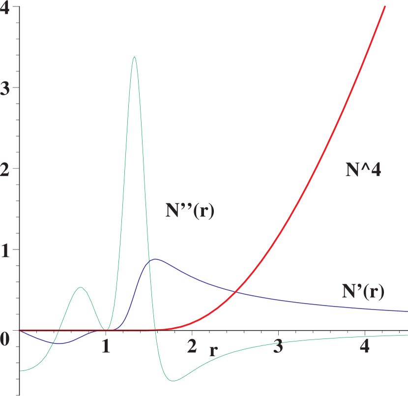
Figure 1: The function $N^{4}(r)$ and the first and second derivatives $N^{\prime}(r)$ and $N^{\prime\prime}(r)$. The images are at the rescaled radius $r=1$.

Figure 1 illustrates the function $N^{4}(r)$ and the first and second derivatives of $N(r)$.

The potential $\phi_{\nu}$ is designed to have the following property: It dominates the stellar potential $\phi_{*}(R)$ at radii much larger than the Einstein radius $R_{E}$ with

$$\phi_{\nu}\sim m_{0}\nu\ln^{4}(R/R_{E}),\qquad\phi_{*}(R)\sim(1-\nu)m_{0}\ln(R/R_{E}).$$ (11)

But at small radius $\phi_{n}u$ is small and has virtually no effect on lensing. In particular, it keeps the convergence $\kappa$, shear $\gamma$, the components of the amplification matrix $\mu$ and the time delay between images unchanged at the radii of the four images $R=R_{i}$. In fact it has a vanishing contribution to the arrival time surface near the images up to the order $O(R-R_{i})^{3}$. This can be verified by Taylor expansion. It is easy to show (also cf. Fig. 1) that the factor $N(r)$ and its first and second radial derivatives obey

$$\left.{N^{\prime\prime}}\right|_{R=R_{i}}=\left.{N}\right|_{R=R_{i}}=\left.{N}\right|_{R=R_{i}}=0.$$ (12)

Becaue $\phi_{\nu}(R)$ is a multiplications of the four $N(r)$, all of the zeroth, first and second derivatives vanish at the four radii $R_{i}$. And because $\phi_{\nu}(R)$ is azimuthally symmetric, all its azimuthal derivatives with respect to $\theta$ also vanish.

The time delay surface

$$\tau(X,Y) = {(X-X_{s})^{2}+(Y-Y_{s})^{2}\over 2}$$ (13)

$$- {\gamma_{1}(X^{2}-Y^{2})+2\gamma_{2}XY\over 2}$$

$$- {m_{0}\over\alpha}\ln\left(1+{R^{\alpha}\over R_{e}^{\alpha}}\right)$$

$$- m_{0}\nu\Pi_{i=1}^{4}N\left({R\over R_{i}}\right).$$

Hence when we vary the parameter $\nu$, the time arrival surface $\tau(X,Y)$ yields the same extrema, or images. This means models with different $\nu$ (or halo) will have goodness of fit to all strong lensing data (the time delay, the image positions and even the amplifications and parity of the images). It only alters the mass distribution of the lens, e.g., the total mass of the lens and the spatial extent of the lens. Hence it creates a degeneracy in lens modeling, making it problematic to draw unique conclusions on lens halo mass from image modeling. We note, however, by construction this degeneracy applies only to point images or point sources.

The surface density and mass of the model can be computed as

$$\kappa(R)=1-{1\over 2}\nabla^{2}\tau,\qquad M(R)=R{d\phi\over dR},$$ (14)

in particular, the density and the mass for the stars only are given by

$$\kappa_{*}(R)={\alpha(1-\nu)m_{0}R_{e}^{\alpha}\over 2R^{2-\alpha}(R^{\alpha}+R_{e}^{\alpha})^{2}}$$ (15)

and

$$M_{*}(R)={(1-\nu)m_{0}R^{\alpha}\over R^{\alpha}+R_{e}^{\alpha}}.$$ (16)

As we can see the mass in stars has a half-mass radius $R=R_{e}$, and converges to a finite mass $m_{0}$ at infinity. The density has an inner cusp $2-\alpha$, and drops steeply with radius, by a factor of 25/4 from $R=R_{e}$ to $R=2R_{e}$ for cored models ($\alpha=2$) or by a factor of 4 for isothermal cusped models ($\alpha=0$).

The halo component $\phi_{\nu}(R)$ contributes to $\kappa(0)$ by a negligible amount $\pm 0.001\nu$ for $0\leq R\leq 1.3R_{E}$, but contributes to $\kappa(20R_{E}>R>2R_{E})$ by an amount of the order $\nu R_{E}/R$. This flattens the rotation curve at large radii. A flat rotation curve corresponds to a constant deflection strength,

$$u^{2}\equiv{d\phi\over dR}\equiv{M\over R},$$ (17)

which is effectively the rotation curve squared. At large radius we have

$$M\rightarrow m_{0}+3\nu m_{0}\ln^{3}(R/R_{E}).$$ (18)

In comparsion to the case with only the stars, we have a nearly Keplerian rotation curve beyond $R=2R_{e}$.

3 Results

PG1115+080 is a quadruple system with a nearly axisymmetric stellar lens at $z_{l}=0.31$, and the quasar source is at $z_{s}=1.72$. We use the photometric data of Impey et al. (Impey98 (1998)) for the images A1, A2, B, C, and the time delay $t_{BC}=25$ days between the nearest B image and the furthest C image (Schechter et al. 1997). There is an infared Einstein ring of radius $R_{E}\sim 1.4\arcsec$. The stellar lens is well-approximated by a de Vaucouleurs profile with a half-light radii of $R_{e}=0.55\arcsec=0.4R_{E}$. Since the surface density is nearly cored, we set the cusp slope $2-\alpha=0$. We adopt a $\Lambda$CDM cosmology with the time delay constant for at the redshifts $z_{l}=0.31,z_{s}=1.72$ of PG1115+080 given by

$$100h_{0}^{-1}\zeta(\Omega=1-\Lambda)\sim(30-32)h_{0}^{-1}{\rm day}\,{\rm arcsec}^{-2}.$$ (19)

Let’s try to fit PG1115 with a halo-free model with $\nu=0$. Totally we have five free fitting parameters, with $(\gamma_{1},\gamma_{2},m_{0})$ for the lens model, and $(X_{s},Y_{s})$ being a pair of coordinates for the source. Since the four images provide in general at least eight constraints, we do not expect a perfect fit. Nonetheless a reasonable fit can be found for this star-only model, as shown by the time delay contours in Figure 2a and the cuts in Figure 2b. The model yields a time delay

$$\tau_{BC}\sim 0.56~{}{\rm arcsec}^{2},$$ (20)

between images B and C. Compared with measured delay $t_{BC}=25{~{}\rm day}$, we find

$$h_{0}={100\zeta\tau_{BC}\over t_{BC}}\sim{30\tau_{BC}\over t_{BC}}\sim 0.72$$ (21)

for this star-only model. The high value of $h_{0}$ is related to the very small convergence at the Einstein radius $R_{E}$.

Now consider adding the component $\phi_{\nu}$, i.e., we increase the value $\nu$ from zero to $\nu=0.04,0.08,0.16$. We see no detectable differences in the time delay (cf. Fig. 2a and Fig. 2b), hence we still have $h_{0}=0.72$. All models predict amplification ratios among the four images to be

$$A_{1}:A_{2}:B:C=3:4:0.7:1,$$ (22)

independent of $\nu$. These are in good agreement with the observed infared flux ratios

$$A_{1}:A_{2}:B:C=3.84:2.67:0.64:1,$$ (23)

apart from the well-known problematic flux ratio between the close pair $A_{1}$ and $A_{2}$, which has been attributed to either microlensing or lensing by substructures (e.g., Impey et al. 1998; Barkana 1997; Metcalf & Zhao 2002). Consistent with Kochanek (2002b), our model density is small near $R_{E}$ with a convergence

$$\kappa(R_{E})\sim 0.1+0\times\nu,$$ (24)

independent of $\nu$; by construction $\phi_{\nu}$ has a vanishing contribution to the convergence at the images. But by raising the parameter $\nu$ the models develop a very massive halo at radii $\gg R_{E}$ with a nearly flat rotation curve (cf. Fig. 3), very different from the model with $\nu=0$. This illustrates an explicit counter example to Kochanek’s claim of a conflict between lens models with an extended dark halo and $\Lambda$CDM cosmology with $H_{0}\sim 70$. We do not find such a conflict. Instead we find that the new mass degeneracy prevents us from drawing a robust conclusion about the dark halo on the basis of the image positions and time delays alone.

4 Summary

As we can see, it is possible to construct many very different models with positive, smooth and monotonic surface densities to fit the image positions. There are also no extra images. These models also fit the same time delay and time delay ratios using a Hubble constant and cosmology consistent with $\Lambda$CDM cosmology. Hence the models are truely indistinguishable for lensing data. They fit the flux ratios equally well, and produce nearly indistinguisable Einstein rings, which is the region of minimal gradient of the time delay surface. The models have identical light profiles, undistinguishable by data.

Among the acceptable models to PG1115+080, there are models with a Keplerian rotation curve and models with a nearly flat rotation curve. So lensing data plus $H_{0}$ cannot uniquely specify the mass-to-light ratio of this system.

We conclude that strong lensing data may not uniquely determine the Hubble constant, even if we fix the cosmology, the lens and source redshifts, and the time delays and amplification ratios of the four images. There are at least important degeneracies in inverting the data of a perfect Einstein cross to the lens models and the Hubble constant. The relation between the value of $H_{0}$ and the size of the halo is not straightforward: a high $H_{0}$ does not necessarily mean no dark halo, and models with a flat rotation curve do not always yield a small $H_{0}$. We also comment that it would be difficult to determine the cosmology from strong lensing data alone because the non-uniqueness in the lens models implies that the combined parameter $h_{0}^{-1}\zeta(\Omega,z_{l},z_{s})$ is poorly constrained by the lensing data, even if $h_{0}$ and the redshifts $z_{l},z_{s}$ are given.

This work was supported by the National Science Foundation of China under Grant No. 10003002 and a PPARC rolling grant to Cambridge. HSZ and BQ thank the Chinese Academy of Sciences and the Royal Society respectively for a visiting fellowship, and the host institutes for local hospitalities during their visits.

Table 1: Plausible lens parameters to fit the images of a perfect Einstein cross and time delays with $H_{0}=72$ km/s/Mpc

Size	Mass	Shear	Source	Convergence
$R_{e}/R_{E}$	$m_{0}$	$(\gamma_{1},\gamma_{2})$	$(X_{s},Y_{s})$	$\kappa(0)$	$\kappa(R_{E})$	$\kappa(10R_{E})$	$\kappa(100R_{E})$
0.55/1.4	1.6	(-0.11,0.14)	(-0.05,0.18)	$5.3-1.6\times 10^{-3}\nu$	$10^{-1}$	$10^{-4}+0.3\nu$	$10^{-9}+0.01\nu$

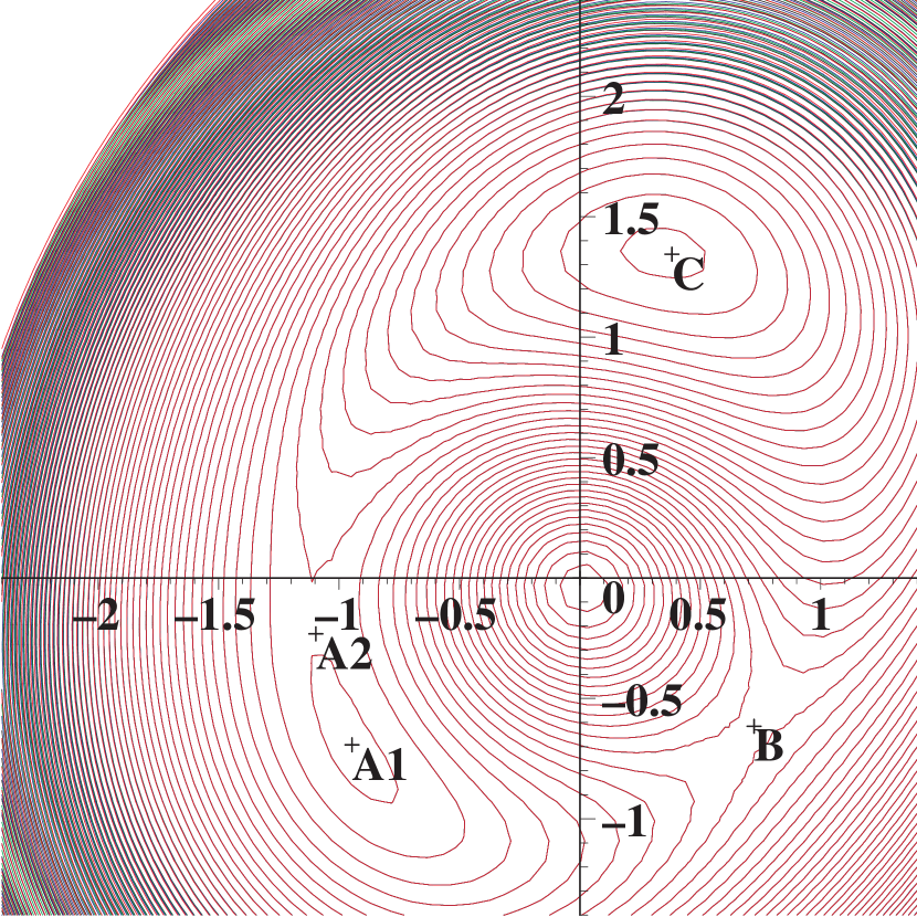
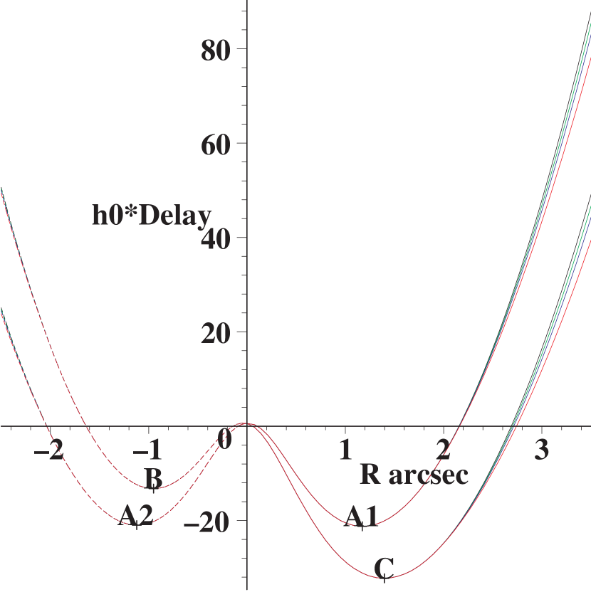
Figure 2: Panel (a) shows time delay contours at intervals of 1 day for the four lens models. All models reproduce the same image positions and time delay with $h_{0}=0.72$. The difference of the models starts to be visible (the contours become thicker) beyond 3 arcsecs from the center. Panel (b) shows cuts of the time delay surfaces of the four lens models along the radial direction from the lens to the time delay minima (marked by “C” and “A1”on solid curves) and from the lens to the saddle images (marked by “B” and “A2” on dashed curves). From bottom to top lines are models with decreasing amount of halos $\nu=0.16,0.08,0.04,0$ with color coded as red, blue, green and black. The measured delay $t_{BC}=25$ days implies $h_{0}=0.72$ for all these models. The time delay ratio $t_{AC}/t_{BA}=1.13\pm 0.18$ of Barkana (1997) is also reproduced.

Figure 3: The deflection strength of the lens $u^{2}={M(R)\over R}={d\phi\over dR}$ as a function of the distance from the lens; this is effectively a rotation curve of the lens. From top right to down right, from thinner to thicker lines are models with decreasing amount of halos $\nu=0.16,0.08,0.04,0$ with color coded as red, blue, green and black. Note that both Keplerian and flat rotation curve models are allowed by the data.

References

- (1) Barkana, R., 1997, ApJ, 489, 21
- (2) Freedman, W.L., Madore, B.F., Gibson, B.K., et al., 2001, ApJ, 553, 47
- (3) Impey, C.D., Falco, E.E., Kochanek, C.S., Lehar, J., McLeod, B.A., Rix, H.-W., Peng, C.Y., & Keeton, C.R., 1998, ApJ, 509, 551
- (4) Kochanek, C.S., 2002a, submitted to ApJ (astro-ph/0204043)
- (5) Kochanek, C.S., 2002b, submitted to ApJ (astro-ph/0205319)
- (6) Kochanek, C.S., 2002c, submitted to ApJ (astro-ph/0206006)
- (7) Metcalf, B., & Zhao, H., 2002, ApJ, 567, L5
- (8) Saha, P., 2000, AJ, 120, 1654
- (9) Saha, P., & Williams, L.L.R., 2001, AJ, 122, 585
- (10) Schechter, P.L., et al., 1997, ApJ, 475, L85
- (11) Williams, L.L.R., & Saha, P., 2000, AJ, 119, 439
- (12) Zhao, H.S., & Pronk, D., 2001, MNRAS, 320, 401
- (13) Zhao, H.S., & Qin B., 2003, ApJ, 582, 000 (in press, Paper I)