Observational Properties of Primordial Stellar Populations

Abstract

We present the first results of a study of the expected properties of the first stellar generations in the Universe. In particular, we consider and discuss a series of properties that, on the basis of the emission from associated HII regions, permit one to discern bona fide primeval stellar generations from the ones formed after pollution from supernova explosions. The expected performance of NGST for the study and the characterization of primordial sources is also discussed.

Cosmology: early universe Cosmology: observations Galaxies: abundance Galaxies: starburst H II regions

0.1 Primordial Stars: Expected Properties

The standard picture is that at zero metallicity the Jeans mass in star forming clouds is much higher than it is in the local Universe, and, therefore, the formation of massive stars, say, 100 M_⊙ or higher, is highly favored. The spectral distributions (SED) of these massive stars are characterized by effective temperatures on the Main Sequence (MS) around $10^{5}$ K (Tumlinson & Shull 2000, Bromm et al. 2001, Marigo et al. 2001). Due to their temperatures these stars are very effective in ionizing hydrogen and helium. It should be noted that zero-metallicity (the so-called population III) stars of all masses have essentially the same MS luminosities as, but are much hotter than their solar metallicity analogues. Note also that only stars hotter than about 90,000 K are capable of ionizing He twice in appreciable quantities, say, more than about 10% of the total He content (e.g. Oliva & Panagia 1983, Tumlinson & Shull 2000). As a consequence even the most massive population III stars can produce HeII lines only for a relatively small fraction of their lifetimes, say, about 1 Myr or about 1/3 of their lifetimes.

The second generation of stars forming out of pre-enriched material will probably have different properties because cooling by metal lines may become a viable mechanism and stars of lower masses may be produced (Bromm et al. 2001). On the other hand, if the metallicity is lower than about $5\times 10^{-4}$Z_⊙, build up of H₂ due to self-shielding may occur, thus continuing the formation of very massive stars (Oh & Haiman 2002). Thus, it appears that in the zero-metallicity case one may expect a very top-heavy Initial Mass Function (IMF), whereas it is not clear if the second generation of stars is also top-heavy or follows a normal IMF.

0.2 Primordial HII Regions

The high effective temperatures of zero-metallicity stars imply not only high ionizing photon fluxes for both hydrogen and helium, but also low optical and UV fluxes. This is because the optical/UV domains fall in the Rayleigh-Jeans tail of the spectrum where the flux is proportional to the first power of the effective temperature, $T_{eff}$, so that, for equal bolometric luminosity, the actual flux scales like $T_{eff}^{-3}$. Therefore, an average increase of effective temperature of a factor of $\sim 2$ will give a reduction of the optical/UV flux by a factor of $\sim 8$. As a result, one should expect the rest-frame optical/UV spectrum of a primordial HII regions to be largely dominated by its nebular emission (both continuum and lines), so that the best strategy to detect the presence of primordial stars is to search for the emission from associated HII regions.

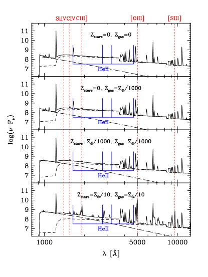
Figure 1: The synthetic spectrum of a zero-metallicity HII region (top panel) is compared to that of HII regions with various combinations of stellar and nebular metallicities (lower panels). The long-dashed and short-dashed lines represent the stellar and nebular continua, respectively.

In Panagia et al.(2002) we report on our calculations using Cloudy90 (Ferland et al.1998) of the properties of primordial, zero-metallicity HII regions (e.g. Figure 1). We find that the electron temperatures is in excess of 20,000 K and that 45% of the total luminosity is converted into the Ly-$\alpha$ line, resulting in a Ly-$\alpha$ equivalent width (EW) of 3000 Å (Bromm, Kudritzki & Loeb 2001). The helium lines are also strong, with the HeII $\lambda$1640 intensity comparable to that of H$\beta$ (Panagia et al.2002, Tumlinson et al.2001).

An interesting feature of these models is that the continuum longwards of Ly-$\alpha$ is dominated by the two-photon nebular continuum. The H$\alpha$/H$\beta$ ratio for these models is 3.2. Both the red continuum and the high H$\alpha$/H$\beta$ ratio could be naively (and incorrectly) interpreted as a consequence of dust extinction even though no dust is present in these systems.

From the observational point of view one will generally be unable to measure a zero-metallicity but will usually be able to place an upper limit to it. When would such an upper limit be indicative that one is dealing with a population III object? According to Miralda-Escudé & Rees (1998) a metallicity Z$\simeq 10^{-3}Z_{\odot}$ can be used as a dividing line between the pre- and post-re-ionization Universe. A similar value is obtained by considering that the first supernova (SN) going off in a primordial cloud will pollute it to a metallicity of $\sim 0.5\times 10^{-3}Z_{\odot}$ (Panagia et al.2002). Thus, any object with a metallicity higher than $\sim 10^{-3}Z_{\odot}$ is not a true first generation object.

Figure 2: Ly-$\alpha$ equivalent widths for HII regions ionized by stars with a range of masses and metallicities. The results obtained for black bodies or stellar atmospheres are very similar.

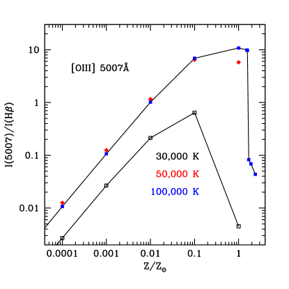
Figure 3: The ratio [OIII]$\lambda 5007$ / H$\beta$ is plotted as a function of metallicity for three different stellar masses: 30,000K (open squares and bottom line), 50,000K (solid diamonds), and 100,000K (solid squares and top line).

0.3 Low Metallicity HII Regions

We have also computed model HII regions for metallicities from three times solar down to $10^{-6}Z_{\odot}$ (Panagia et al. 2002). In Figure 1 the synthetic spectrum of an HII region with metallicity $10^{-3}Z_{\odot}$ (third panel from the top) can be compared to that of an object with zero metallicity (top panel). The two are very similar except for a few weak metal lines. In Figure 2 we show the Ly-$\alpha$ EWs for HII regions ionized by stars with a range of stellar masses and metallicities. Values of EW in excess of 1,000Å are possible already for objects with metallicity $\sim 10^{-3}Z_{\odot}$. This is particularly interesting given that Ly-$\alpha$ emitters with large EW have been identified at z=5.6 (Rhoads & Malhotra 2001).

The metal lines are weak, but some of them can be used as metallicity tracers. In Figure 3 the intensity ratio of the [OIII]$\lambda 5007$ line to H$\beta$ is plotted for a range of stellar temperatures and metallicities. It is apparent that for $Z<10^{-2}Z_{\odot}$ this line ratio traces metallicity linearly. Our reference value $Z=10^{-3}$ corresponds to a ratio [OIII]/H$\beta$ = 0.1. The weak dependence on stellar temperature makes sure that this ratio remains a good indicator of metallicity also when one considers the integrated signal from a population with a range of stellar masses.

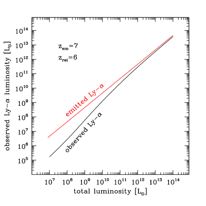
Figure 4: Transmitted Ly-$\alpha$ intensity as a function of the object luminosity. Bright objects ionize their neighborhood and are able to reduce the Ly-$\alpha$ attenuation.

Another difference between zero-metallicity and low-metallicity HII regions lies in the possibility that the latter may contain dust. For a $Z=10^{-3}Z_{\odot}$ HII region dust may absorb up to 30 % of the Ly-$\alpha$ line, resulting in roughly 15 % of the energy being emitted in the far IR (Panagia et al. 2002).

0.4 How to discover and characterize Primordial HII Regions

It is natural to wonder whether primordial HII regions will be observable with the generation of telescopes currently on the drawing boards. In this section we will focus mostly on the capabilities of the Next Generation Space Telescope.

Before proceeding further we have to include he effect of HI absorption in the IGM on the Ly-$\alpha$ radiation (Miralda-Escudé & Rees 1998, Madau & Rees 2001, Panagia et al.2002). A comparison of the observed vs emitted Ly-$\alpha$ intensities is given in Figure 4. The transmitted Ly-$\alpha$ flux depends on the total luminosity of the source since this determines the radius of the resulting Strömgren sphere. A Ly-$\alpha$ luminosity of $\sim 10^{10}$ L_⊙ corresponds to $\sim 10^{6}$ M_⊙ in massive stars. In the following we will consider this as our reference model.

The synthetic spectra, convolved with suitable filter responses can be compared directly to the NGST imaging sensitivity for $4\times 10^{5}$s exposures (see Figure 5). It is clear that NGST will be able to easily detect such objects. Due to the high background from the ground, NGST will remain superior even to 30m ground based telescopes for these applications.

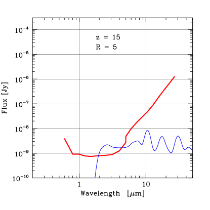
Figure 5: Synthetic spectral energy distribution of a Z=$10^{-3}Z_{\odot}$ starburst object at z=15 containing $10^{6}$ M_⊙ in massive stars (thin line) compared to the imaging limit of NGST at R=5 (thick line). The NGST sensitivity refers to $4\times 10^{5}$ s exposures with S/N=10t.

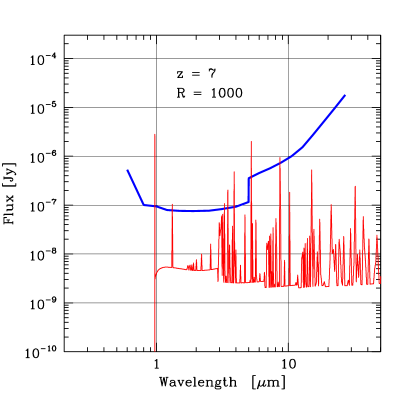
Figure 6: Synthetic spectrum of a Z=$10^{-3}Z_{\odot}$ starburst object at z=7 containing $10^{6}$ M_⊙ in massive stars (thin line) compared to the spectroscopic limit of NGST at R=1000 (thick line). The NGST sensitivity refers to $4\times 10^{5}$ s exposures with S/N=10.

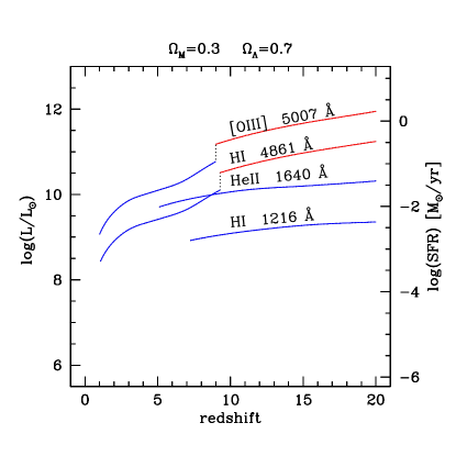
Figure 7: Limiting total luminosity of the ionizing stars (left-hand scale) and top-heavy IMF star formation rate (right-hand scale) to detect various emission lines using NGST spectroscopy, with S/N=10 in integrations of 100 hours, as a function of the source redshift.

The synthetic spectra can also be compared to the NGST spectroscopic sensitivity for $4\times 10^{5}$s exposures (see Figure 6): it appears that while the Ly-$\alpha$ line can be detected up to redshifts as high as 15 or 20, for our reference source only at relatively low redshifts (z$\sim 7$), can NGST detect other diagnostics lines lines such as HeII 1640Å, and Balmer lines. Determining metallicities is then limited to either lower redshifts or to brighter sources.

We can reverse the argument and ask ourselves what kind of sources can NGST detect and characterize with spectroscopic observations. Figure 7 displays, as a function of redshift, the total luminosity of a starburst whose lines can be detected with a S/N=10 adopting an exposure time of $4\times 10^{5}$s. The loci for Ly-$\alpha$, HeII 1640Å, H$\beta$, and [OIII] 5007Å are shown. It appears that Ly-$\alpha$ is readily detectable up to z$\simeq$20, HeII 1640Å may also be detected up to high redshifts if massive stars are indeed as hot as predicted, whereas “metallicity” information, i.e. the intensity ratio I([OIII])/I(H$\beta$), can be obtained at high redshifts only for sources that are 10–100 times more massive or that are 10–100 times magnified by gravitational lensing.

0.5 Conclusions

We have considered and discussed a series of properties that, on the basis of the emission from associated HII regions, permit one to discern bona fide primeval stellar generations from the ones formed after pollution from supernova explosions. We find that it is possible to discern truly primordial populations from the next generation of stars by measuring the metallicity of high-z star forming objects. The very low background of NGST will enable it to image and study first-light sources at very high redshifts, whereas its relatively small collecting area olimits its capability in obtaining spectra of z$\sim$10–15 first-light sources to either the bright end of their luminosity function or to strongly lensed sources.

References

- [1] Baraffe, I., Heger, A., & Woosley, S.E. 2001, ApJ, 550, 890
- [2] Bromm, V., Ferrara, A., Coppi, P.S., & Larson, R.B. 2001, MNRAS, 328,969
- [3] Bromm, V., Kudritzki, R.P., & Loeb, A. 2001, ApJ, 552, 464
- [4] Ferland, G.J., Korista, K.T., Verner, D.A., Ferguson, J.W., Kingdon, J.B., & Verner E.M. 1998, PASP, 110, 761
- [5] Gunn, J.E., & Peterson, B.A. 1965, ApJ, 142, 1633
- [6] Heger, A., & Woosley, S.E. 2002, ApJ, 567, 532
- [7] Izotov, Y.I., & Thuan, T.X. 1998, ApJ, 500, 188
- [8] Madau, P., & Rees, M.J. 2001, ApJ, 551, L27
- [9] Marigo, P., Girardi, L., Chiosi, C., & Wood, P.R. 2001, A&A 371, 252
- [10] Miralda-Escudé, J., & Rees, M.J. 1998, ApJ, 497, 21
- [11] Oh, S.P., & Haiman, Z. 2002, ApJ, 569, 558
- [12] Oliva, E., & Panagia, N. 1983, Ap&SS, 94, 437
- [13] Panagia, N., Stiavelli, M., Ferguson, H.C., & Stockman, H.S. 2002, in preparation
- [14] Rhoads, J.E., & Malhotra, S. 2001, ApJ, 563, L5
- [15] Tumlinson, J., & Shull, J.M. 2000, ApJ, 528, L65
- [16] Tumlinson, J., Giroux, M.L., & Shull, J.M. 2001, ApJ, 550, L1