Notch Filter Masks:
Practical Image Masks for Planet-Finding Coronagraphs

Abstract

An ideal coronagraph with a band-limited image mask can efficiently image off-axis sources while removing identically all of the light from an on-axis source. However, strict mask construction tolerances limit the utility of this technique for directly imaging extrasolar terrestrial planets. We present a variation on the basic band-limited mask design—a family of “notch filter” masks—that mitigates this problem. These robust and trivially achromatic masks can be easily manufactured by cutting holes in opaque material.

1 INTRODUCTION

Direct optical imaging of nearby stars has emerged as a potentially viable method for detecting extrasolar terrestrial planets, buoyed by new techniques for controlling diffracted and scattered light in high-dynamic-range space telescopes (see, e.g., the review by Kuchner & Spergel 2003). These techniques boost a telescope’s ability to separate a planet’s light from the light of its host star. At optical wavelengths, the Sun outshines the Earth by a factor of nearly $10^{10}$; this contrast ratio is $\sim 10^{3}$ times larger than the contrast ratio in the mid-infrared (Beichman et al., 1999; Des Marais et al., 2001). But to offset the higher dynamic range requirements of visible-light planet finding, optical techniques offer freedom from large, multiple-telescope arrays (Woolf, 2003), cryogenic optics, and background light from zodiacal and exozodiacal dust (Kuchner & Brown, 2000), while providing access to $O_{2}$ and $O_{3}$ biomarkers (Traub & Jucks, 2001; Des Marais et al., 2001), surface features (Ford, Seager & Turner, 2001), the total atmospheric column density (Traub, 2003), and even potentially the “red edge” signal from terrestrial vegetation (Woolf et al., 2002).

Of the obstacles to achieving the necessary dynamic range in a single-dish optical telescope, the diffracted light background appears relatively manageable. For example, maintaining the scattered light background at the level of the expected signal from the planet poses a greater challenge; this task requires a r.m.s. wavefront accuracy of $\lesssim 1$ Å (Kuchner & Traub, 2002; Trauger et al., 2002a) over the critical spatial frequencies. However, techniques for managing the diffracted light may dictate the general design of a planet-finding telescope and the planet search and characterization strategy.

Optical techniques for controlling diffracted light in planet-imaging telescopes have centered on two main designs: specially shaped and/or apodized pupils (Spergel, 2001; Nisenson & Papaliolios, 2001; Kasdin, Spergel & Littman, 2001; Debes et al., 2002; Kasdin et al., 2003) and classical coronagraphs (Lyot, 1939; Nakajima, 1994; Stahl & Sandler, 1995; Malbet et al., 1995; Kuchner & Traub, 2002). Shaped and apodized pupils produce a point spread function whose diffraction wings are suppressed in some regions of the image plane. A classical coronagraph explicitly removes the on-axis light from the optical train by reflecting or absorbing most of it with an image mask and diffracting the remainder onto an opaque Lyot stop.

Recently, Kuchner & Traub (2002) showed that a classical coronagraph performs best with a “band-limited” image mask. Different band-limited masks offer high performance for planet searching or planet characterization. For planet characterization, the $\sin^{2}$ amplitude transmissivity mask ($\sin^{4}$ intensity transmissivity) introduced in Kuchner & Traub (2002) can achieve 80% throughput for a planet at 4$\lambda/D$. With this high throughput, a 10 m by 4 m telescope can detect a planetary biomarker in $\sim$1/3 of the time needed by alternative designs (e.g., an 8 m square apodized aperture). A band-limited mask of the form $1-{\rm sinc}$ (see Table 1) has both excellent throughput and large search area. With any band-limited mask, an ideal coronagraph eliminates identically all of the on-axis light, though pointing errors and the stellar size contribute to a finite leakage (Kuchner & Traub, 2002). A band-limited mask can operate with a pupil of any shape as long as it has uniform transmissivity.

But because they interact with focused starlight, all coronagraphic image masks face severe construction tolerances. Errors in the mask intensity transmissivity of $\sim 10^{-9}$ on scales of $\lambda/D$ near the center of the mask can scatter enough light into the field of view to scuttle a planet search (Kuchner & Traub, 2002). Painting a graded-transmissivity mask requires a steady hand! This requirement has cast the classical coronagraph in an unfavorable light, despite its potential high performance and flexibility.

In this paper, we offer a way around this pitfall of classical coronagraphy: an easy-to-manufacture class of image masks. We illustrate a family of binary image masks which offer a savings in construction tolerances of $\sim 5$ orders of magnitude compared to graded image masks, analogous to the advantage of using binary rather than graded pupil masks (Spergel, 2001). These “notch filter” masks offer the same planet search and characterization advantages as ideal band-limited masks, providing a robust, practical means of controlling diffracted light in a planet-finding coronagraph.

2 BAND-LIMITED MASKS

We begin by reviewing the theory of band-limited image masks. We retain the notation of Kuchner & Traub (2002); image plane quantities have hats and pupil plane quantities do not.

Figure 1 illustrates schematically how a coronagraph works; light passes through the pupil and converges on an image mask, then the pupil is re-imaged onto a Lyot stop. Starlight focused on the center of the image mask diffracts to the pupil edges, where the Lyot stop can block it, as shown on the left of the figure. Light from an off-axis planet diffracts all around the second pupil plane, as shown on the right of the figure, and largely passes through the Lyot stop.

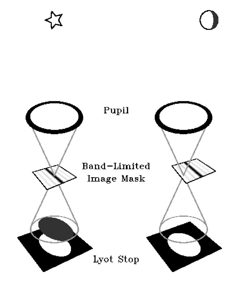
Figure 1: Cartoon of a coronagraph with a band-limited image mask. The image mask diffracts on-axis starlight to a region restricted to the edges of the pupil plane, where a Lyot stop blocks it. Off-axis light from a planet diffracts all around the pupil plane, and through the center of the Lyot stop.

A band-limited mask has a transmission function chosen to diffract all the light from an on-axis source to angles within $\epsilon D/(2\lambda)$ of the edges of the pupil, as shown in Figure 1, so that a well-chosen Lyot stop can block identically all of that diffracted light. Such an image mask typically consists of a series of dark rings or stripes. The parameter, $\epsilon$, is the bandwidth of the mask.

A mask can be described by an amplitude transmissivity, $\hat{M}(x,y)$, and intensity transmissivity $|\hat{M}(x,y)|^{2}$ where $x$ and $y$ are cartesian coordinates in the image plane. Image masks are generally opaque ($\hat{M}=0$) in the center ($x=y=0$) and close to transparent ($\hat{M}\approx 1$) away from the center, in the search area. To understand the need for band-limited pupil masks, we must examine the Fourier transform of $\hat{M}(x,y)$, given by

$$M(u,v)=\int\!\!\int\hat{M}(x,y)\,e^{-2\pi i(ux+vy)}\,dx\,dy$$ (1)

The amplitude transmissivity of a completely transparent mask has only one Fourier component, at zero frequency, i.e. $M(u,v)=\delta(u,v)$.

Figure 2 illustrates the operation of a mask with one cosine component besides the zero-frequency component, the $\sin^{2}$ mask ($\sin^{4}$ intensity transmissivity) described in Kuchner & Traub (2002). The Fourier transform of the amplitude transmissivity of this mask consists of three delta functions:

$$M(u,v)=-{1\over 4}\delta(u+\epsilon D/(2\lambda),v)+{1\over 2}\delta(u,v)-{1\over 4}\delta(u-\epsilon D/(2\lambda),v)$$ (2)

This mask is the simplest example of a band-limited mask.

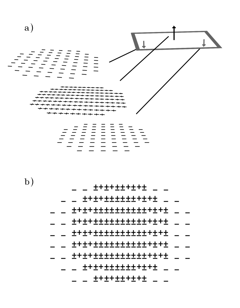
Figure 2: Convolving the pupil field of an on-axis source with the Fourier transform of $\sin^{2}$. a) For each delta function in the Fourier transform, there is one weighted copy of the field, a virtual pupil. b) The field in the second pupil plane is the sum of the fields of the virtual pupils. The fields cancel to zero in the center where there are equal densities of plus and minus signs.

The amplitude transmissivity, $\hat{M}(x,y)$, multiplies the field amplitude in the image plane. In the pupil plane, on the other side of a Fourier transform, this multiplication becomes a convolution. Figure 2a illustrates the convolution of the amplitude of the pupil field of an monochromatic on-axis source and the function, $M(u,v)$, given in Equation 2.

In the convolution, each $\delta$-function from Equation 2 generates a weighted copy of the pupil field—a virtual pupil. We represent each copy of the field as a circle filled with $+$ signs or $-$ signs. The circular shape represents a circular aperture, though any aperture shape will do. Since the central $\delta$-function has twice the weighting of the other $\delta$-functions, the $+$ signs have twice the density of the $-$ signs in Figure 2a.

Figure 2b depicts the field in the second pupil plane, the sum of the three virtual pupil fields shown in Figure 2a. In the center of Figure 2b, the densities of $+$ and $-$ signs are equal; for every $+$ sign, there is a $-$ sign. In this region, the fields cancel to zero. Elsewhere the fields do not cancel. The next optical element in the coronagraph beam train is a Lyot stop, which transmits light in the center of the pupil plane, but blocks the regions where the fields do not cancel.

A given Lyot stop blocks the light diffracted by a range of Fourier components. If the the Lyot stop blocks a fraction, $\epsilon$, of the pupil radius at the pupil edges, it will block the diffracted light from all spatial frequency components in the mask with spatial frequency $|u|<\epsilon D/(2\lambda)$, where $D$ is the telescope diameter, and $\lambda$ is the wavelength. One can create a mask which contains any or all of the cosine Fourier components at these low frequencies which the Lyot stop will still match; this family of masks which has power in only a limited range of low spatial frequencies is the family of band-limited masks. We can use $\epsilon$ to refer to the bandwidth of a Lyot stop or the bandwidth of an image mask matched to that Lyot stop.

Likewise, a given ideal Lyot stop and mask combination can work at a range of wavelengths. The bandwidth of a given image mask is proportional to $\lambda$, but the bandwidth of a given Lyot stop is independent of $\lambda$. Therefore, a given Lyot stop/image mask combination will work at all wavelengths shorter than the wavelength for which it was designed. However, it can only have optimum throughput at one wavelength.

Kuchner & Traub (2002) display a variety of one-dimensional band-limited mask amplitude transmissivity functions. A useful compromise between search area and throughput is $\hat{M}(x)=N\left(1-{\rm sinc}(\pi x\epsilon D/\lambda)\right)$, where ${\rm sinc}\,{x}=\sin(x)/x$, and $1-1/N$ is the minimum value of ${\rm sinc}\,{x}$ (i.e., $N=0.82153497637881...$). The throughput of a Lyot stop matched to a one-dimensional mask function is roughly $1-\epsilon$. Band-limited masks with additional Fourier components in the $v$ direction are also possible, though to use these masks, one must stop the top and bottom of the pupil plane as well as the left and right. The throughput of such a Lyot stop is roughly $(1-\epsilon)^{2}$.

At the request of NASA, a university-industry team associated with Ball Aerospace and Technologies Corporation studied a design for a space-based visible-light planet finding telescope using a single 4 m by 10 m elliptical primary mirror. This team estimated that with a classical coronagraph using a Gaussian image mask, the design could detect an Earth twin orbiting a G2 V star at a distance of 10 pc in 0.86 hours, including time for 2 rotations of the image plane (Beichman et al., 2002). Once the location of the planet was known, a water band in the planet’s atmosphere could be detected spectroscopically in 0.14 days, and an $O_{2}$ band could be detected in 0.8 days. If a single band-limited image mask of the form $\hat{M}(x)=1-{\rm sinc}^{2}{x}$ were used instead of a Gaussian mask, the Lyot stop could be substantially widened, increasing the throughput, and the detection and characterization times would be reduced by a factor of roughly 0.7, to 0.6 hours for detection, 0.1 days for $H_{2}O$, and 0.6 days for $O_{2}$.

Ideally, a band-limited mask combined with a Lyot stop completely blocks all on-axis starlight from reaching the second image plane, and attenuates off axis starlight to an easily manageable level. However, Kuchner & Traub (2002) discuss two significant limitations on the band-limited mask performance: pointing errors and errors in mask construction. None of the time estimates in the Ball report accounts for either of these errors, which affect all masks, band-limited or not.

A mildly apodized Lyot stop can compensate for the leakage due to pointing errors (Kuchner & Traub, 2002). Apodizing the Lyot stop carries a throughput penalty, but even with this loss, the ideal classical coronagraph outfitted with a choice of band-limited masks remains by far the fastest of the idealized designs described in the Ball report for planet detection. Mask errors are more serious; all graded image masks suffer from impractically tight construction tolerances. We will show how to dramatically loosen the construction requirements by building binary masks.

3 NOTCH FILTER MASKS

To build a binary mask that retains the advantages of band-limited masks we will need to use more of the available function space for mask design. Section 2 reviewed the utility of masks whose Fourier components are limited to spatial frequencies $|u|<\epsilon D/(2\lambda)$. However, there is another range of spatial frequencies available for mask design: as Kuchner & Traub (2002) described in their discussion of mask errors, high spatial frequency terms that diffract light well outside the opening in the Lyot stop do not affect the performance of a mask. We can add high spatial-frequency terms, with $|u|>(1-\epsilon/2)(D/\lambda)$, to the mask amplitude transmissivity function without altering the light admitted through the coronagraph as long as

$$\int_{-\epsilon D/(2\lambda)}^{\epsilon D/(2\lambda)}M(u)\,du=0.$$ (3)

Figure 3 shows that the spatial frequency response of a general image mask which can completely suppress on-axis light resembles the spectral response of a notch filter.

Figure 3: Power spectra of a band-limited mask (a) and a notch filter mask (b). The mask functions may have power at spatial frequencies indicated by the hatched regions.

We can use the degrees of freedom available at high spatial frequencies to design masks which are relatively easy to construct to the necessary tolerances. For example, the transmissivity of a band-limited mask is analytic, so it can not have a constant value over any finite region. However, the transmissivity of a notch filter mask need not obey this restriction. The remainder of this paper will be a discussion of notch filter masks that take advantage of this opportunity.

4 ONE-DIMENSIONAL MASK FUNCTIONS

Sampling a function forces its Fourier transform to be periodic. We can harness this aliasing effect to generate useful notch filter mask functions. We will illustrate this principle first by considering mask functions of one variable only. Such a mask function can be realized as a striped mask as shown in Kuchner & Traub (2002). These functions can also be used as parts to construct two-dimensional masks.

Throughout our discussion, $\hat{M}_{BL}(x)$ will be a function which can serve as the amplitude transmissivity of a band-limited mask: $0\leq\hat{M}_{BL}(x)\leq 1$, $\hat{M}_{BL}(0)=0$, and the Fourier transform, $M_{BL}(u)$, of this function only has power at spatial frequencies $u<\epsilon D/(2\lambda)$. Such a function automatically satisfies Equation 3. We shall use $\hat{M}_{BL}(x)$ to create notch filter functions, $\hat{M}_{notch}(x)$, that mimic $\hat{M}_{BL}(x)$ at low spatial frequencies.

4.1 Sampling

Actual image masks are constructed using finite-sized tools offering limited contrast and spatial resolution. We can design notch filter masks with this contraint in mind. Multiply $\hat{M}_{BL}(x)$ by a comb filter with spacing $\Delta x$ to get a sampled version of $\hat{M}_{BL}(x)$, and convolve the result with a function $\hat{P}(x)$, to get

$$\hat{M}_{sampled}(x) = \hat{P}(x)*\left(\hat{M}_{BL}(x)\,{\Delta x}\sum_{n}\delta(x-(n+\zeta)\Delta x)\right)$$ (4a)

$$M_{sampled}(u) = P(u)\left(M_{BL}(u)*\sum_{n}\delta(u-n/\Delta x)e^{-2\pi iu\zeta\Delta x}\right),$$ (4b)

where $n$ ranges over all integers and $*$ indicates convolution. For generality, we have allowed the sampling points to be offset from the mask center by a fraction $\zeta$ of $\Delta x$. The kernel, $\hat{P}(x)$, can represent the “beam” of a nanofabrication tool. It should be normalized so that $\int_{-\infty}^{\infty}\hat{P}(x)\,dx=1$, and $\hat{P}(x)$ must be everywhere $\leq 1/(\Delta x)$, so $\hat{M}_{sampled}(x)$ remains $\leq 1$.

This function we have created, $M_{sampled}(u)$, only has power at $|u-n/{\Delta x}|<\epsilon/2$. Its power spectrum resembles Figure 3 as long as the spacing between the samples satisfies the requirement

$$\Delta x\leq\lambda/D.$$ (5)

If $\zeta\neq 0$, then $M_{sampled}(u)$ typically has an imaginary component. However, if Equation 5 holds, $M_{sampled}(u)$ is always purely real at low frequencies ($u<\epsilon D/(2\lambda)$).

In general, $M_{sampled}(u)$ does not match $M_{BL}(u)$ at low frequencies, because the envelope function, $P(u)$, in Equation 4b does not generally equal unity over the whole bandwidth of $\hat{M}_{BL}(x)$. Rather, the envelope function tends to cause $M_{sampled}(u)$ to violate Equation 3. However, we can often correct for this effect and create a function, $M_{notch}(u)$, which satisfies Equation 3 by subtracting a constant, $\hat{M}_{0}$, from $\hat{M}_{sampled}(x)$. I.e.,

$$\hat{M}_{notch}=\hat{M}_{sampled}-\hat{M}_{0},$$ (6)

where

$$\hat{M}_{0}=\int_{-\epsilon D/(2\lambda)}^{\epsilon D/(2\lambda)}M_{sampled}(u)\,du=\int_{-\infty}^{\infty}M_{BL}(u)P(u)\,du=\left.\hat{M}_{BL}(x)*\hat{P}(x)\right|_{x=0}.$$ (7)

To use this technique, we must not sample $\hat{M}_{BL}(x)$ where $\hat{M}_{BL}(x)=0$, or else we will end up specifying a mask with $\hat{M}_{notch}(x)<0$. Specifically, $|\zeta|$ must be greater than some minimum value, $\zeta_{0}$, given by the condition that $\hat{M}_{BL}(\zeta_{0}\Delta x)=\hat{M}_{0}$. We may symmetrize the mask if we desire by forming a combination such as $(\hat{M}_{notch}(x)+\hat{M}^{\prime}_{notch}(x))/2$, or $\hat{M}_{notch}(x)\hat{M}^{\prime}_{notch}(x)$ where for $\hat{M}^{\prime}_{notch}(x)$, $-\zeta$ has been substituted for $\zeta$. The latter combination has twice the bandwidth of the former.

For example, if we choose $\Delta x=\lambda/D$, and $\hat{P}(x)=({D}/{\lambda})\Pi(xD/\lambda)$, where $\Pi(x)$ is a tophat function,

$$\Pi(x)=\left\{\begin{array}[]{ll}1&\mbox{where $-1/2<x<1/2$ }\\ 0&\mbox{elsewhere},\end{array}\right.$$ (8)

then $P(u)={\rm sinc}(\pi u\lambda/D)$, and our sampling algorithm generates a mask resembling a histogram plot. A graded version of this mask would consist of stripes of different uniform shadings. Choosing $\zeta=\zeta_{0}$ will generate a striped mask whose darkest stripe is perfectly opaque. Choosing $\zeta_{0}>\zeta\leq 0.5$ will generate a striped mask which never becomes perfectly opaque, a potentially useful trick since fabricating graded masks with high optical densities can be a challenge (Wilson et al., 2002).

If $\hat{M}_{BL}(x)=\sin^{2}(\pi x\epsilon D/(2\lambda))$, then Equation 7 tells us that for this mask, $\hat{M}_{0}=(1/2)(1-{\rm sinc}(\pi\epsilon/2))$, and $\zeta_{0}$ is given by the condition $\hat{M}_{BL}(\zeta_{0}\lambda/D)=\hat{M}_{0}=\sin^{2}(\pi\zeta_{0}\epsilon/2)$. The trick probably only works for the $\sin^{2}$ mask when $\epsilon=1/n$, since $\sin^{2}$ has so many zeros. Table 1 lists $\hat{M}_{0}$ and $\zeta_{0}$ for several other masks, given a tophat kernel.

Table 1: Sampled Mask Parameters for $\hat{P}(x)=({D}/{\lambda})\Pi(xD/\lambda)$

$\hat{M}_{BL}(x)$	$\hat{M}_{0}(\epsilon)$	$\epsilon$	$\hat{M}_{0}$	$\zeta_{0}$
$\sin^{2}{{\pi x\epsilon D}\over{2\lambda}}$	${1\over 2}\left[1-{\rm sinc}(\pi\epsilon/2)\right]$	0.2	0.0081842	0.2883579
		0.4	0.0322554	0.2873981
$N\left[1-{\rm sinc}{{\pi x\epsilon D}\over{\lambda}}\right]$	${N\over 2}\left[1-{2\over\epsilon}\int_{0}^{\epsilon/2}{\rm sinc}(\pi u^{\prime})\,du^{\prime}\right]$	0.2	0.0022456	0.2039059
		0.4	0.0089032	0.2032511
$1-\left({\rm sinc}{{\pi x\epsilon D}\over{2\lambda}}\right)^{2}$	${1\over 2}\left[1-{4\over\epsilon}\int_{0}^{\epsilon/2}(1-{{2u^{\prime}}\over{\epsilon}}){\rm sinc}(\pi u^{\prime})\,du^{\prime}\right]$	0.2	0.0013681	0.1019893
		0.4	0.0054400	0.1017713

Figure 4 shows five examples of notch filter masks all of which are different versions of the same basic $1-{\rm sinc}$ mask. Figure 4a is a simple band-limited mask with no additional high-frequency components. Figure 4b shows a version of this mask sampled as described above with a tophat kernel of width $\lambda/D$. This kernel is the narrowest one that works with $\Delta x=\lambda/D$; narrower kernels require finer samplings.

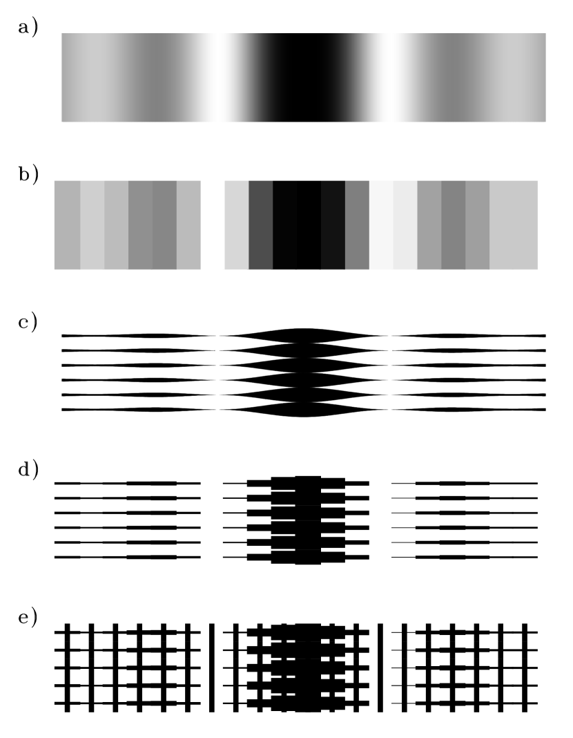
Figure 4: Close-up view of the center of a one-dimensional linear graded band-limited mask (a), and four notch-filter versions of this design (b,c, d, and e).

5 BINARY MASKS

In two dimensions, we can use the additional degrees of freedom afforded by the high-frequency terms in a notch filter function to generate a completely binary mask, i.e., a mask which everywhere satisfies $\hat{M}_{binary}(x,y)=0$ or $\hat{M}_{binary}(x,y)=1$. Such a mask can be constructed entirely out of material which is highly opaque, like metal foil.

5.1 Linear Binary Masks

Let

$$\hat{M}_{stripe}(x,y)=\left\{\begin{array}[]{ll}0&\mbox{where $|y|<\hat{M}_{notch}(x)\lambda/(2D)$ }\\ 1&\mbox{elsewhere}\end{array}\right.$$ (9)

and

$$\hat{M}_{binary}(x,y)=\left(\sum_{n}\delta(y-n\lambda/D)\right)*\hat{M}_{stripe}(x,y).$$ (10)

The Fourier transform of this convolution is a product:

$$\hbox{\hskip-18.06749pt}M_{binary}(u,v) = \left({{D}\over{\lambda}}\sum_{n}\delta(v-nD/\lambda)\right)\int\!\!\int\hat{M}_{stripe}(x,y)e^{-2\pi i(ux+vy)}\,dx\,dy$$ (11)

$$= \left(\sum_{n}\delta(v-nD/\lambda)\right)\int{\rm sinc}(\pi v(\lambda/D)\hat{M}_{notch}(x))\hat{M}_{notch}(x)e^{-2\pi iux}\,dx.$$

At low and mid-spatial frequencies, only the $v=0$ term contributes, and

$$M_{binary}(u,v)=M_{notch}(u)\approx M_{BL}(u)\qquad\mbox{for $u,v<\epsilon D/(2\lambda)$}.$$

Though $\hat{M}_{notch}(x)=1$ in some places, it is possible to multiply $\hat{M}_{notch}(x)$ by a positive real constant, less than 1, to allow for a mask substrate that is not perfectly transparent or reflective, or to guarantee that the metal strips maintain at least a minimum width, at a small cost in throughput.

If we use a sampled mask function for $\hat{M}_{notch}(x)$, the binary mask may be constructed entirely from opaque rectangles of varying lengths, for example, generating a “manhattan” pattern for simple nanofabrication. Figures 4c, d and e show examples of binary masks which mimic the $1-{\rm sinc}$ mask. Figures 4d and e are binary sampled masks.

5.2 Circular Binary Masks

We recommend using a linear mask for the following reasons: 1) Linear masks have bandwidth in one direction only, so they generally have the best throughput. 2) If one region of the mask deteriorates, the mask may simply be translated so that the starlight falls on a new region. 3) Errors in the uniformity of the wavefront in the direction perpendicular to the image mask cancel out in the Lyot plane; for example, the telescope need only be pointed accurately in one direction. 4) It may be possible to use a carefully oriented linear mask to block the light from a binary star.

However, circularly symmetric image masks can provide slightly more search area than linear image masks, so we discuss them here. Figure 5a shows the center of a graded band-limited mask of the form $\hat{M}_{BL}(r)=N(1-{\rm sinc}\,{\pi r\epsilon D/\lambda})$. Figure 5b shows a sampled version of this mask, where, necessarily, the sampling has been performed in two-dimensions. Creating this sampled mask requires following the same procedure illustrated in Section 4.1 to guarantee that the mask satisfies Equation 3. The sample points are shifted by a fraction of $\lambda/D$ in some direction, and a constant is subtracted from the mask amplitude transmissivity.

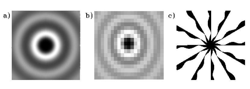
Figure 5: Close-up view of the center of a one-dimensional radial band-limited mask (a), and two equivalent notch-filter versions (b and c).

We can also replace an azimuthally symmetric transmission function, $\hat{M}(r)$, with a discrete K-fold symmetric “star” mask. First, choose a 1-dimensional band-limited function, $\hat{M}(r)_{BL}$ or a notch filter version, $\hat{M}_{notch}(r)$. Then let

$$\hat{M}_{binary}(r,\theta)=\left\{\begin{array}[]{ll}1&\mbox{where ${\rm mod}(K\theta/2\pi,1)<\hat{M}_{notch}(r)$ }\\ 0&\mbox{elsewhere}\end{array}\right.$$ (12)

The Fourier transform of this function (see, e.g., Jackson (1975), p131 [problem 3.14]) is

$$M_{binary}(q,\phi)=\hbox to0.0pt{$\displaystyle\int_{0}^{\infty}\hat{M}(r)J_{0}(qr)r\,dr$\hss}$$ (13)

$$+\sum_{m=-\infty}^{m=\infty}i^{m}\exp(imK\phi)\int_{0}^{\infty}J_{mK}(qr)\sin(m\hat{M}_{notch}(r))r\,dr$$

where $q$ and $\phi$ are the radial and angular polar coordinates in the pupil plane, and $J_{m}$ is the Bessel function of order $m$. Figure 5c shows an example of such a binary star mask.

For a truely band-limited mask, the radial integrals in Equation 13 should be evaluated over a range from 0 to infinity. However, as Kuchner & Traub (2002) discussed, a mask truncated at a radius of say, $r=100\lambda/D$, can serve more than adequately as an approximation to a band-limited mask. Moreover, the mask illumination falls off rapidly with $r$, so deviations from an ideal mask are inconsequential outside some radius $r_{max}$, which is likely to be much less than $100\lambda/D$.

If we consider the mask to be truncated at $r=r_{max}$, the high frequency terms are significant only for high $q$. Since $J_{mK}(qr)\approx(qr)^{mK}/(2^{mK}(mK)!)$ for $qr<mK$, the higher order terms must have absolute values less than $(Dr_{max}/(4\lambda))^{K}/K!$ inside the pupil ($q\leq D/(2\lambda)$); with enough points in the star, these terms are all small. For example, if $r_{max}=10\lambda/D$, $\hat{M}$ will be less than $10^{-5}$ interior to the Lyot stop for $K\geq 14$; this level suffices to allow a coronagraph to suppress the intensity of an on-axis source in the final image plane by a factor of $10^{-10}$.

5.3 Combining Notch Filter Masks

In general, the product of two notch filter mask functions is not a notch filter mask function. However, all of the examples of notch filter mask functions discussed in this paper—except for the circular masks—have periodic Fourier transforms. The product of two such functions is another periodic notch filter function. For example, one notch filter mask is

$$\hat{M}_{binary}(x,y)=\left\{\begin{array}[]{ll}0&\mbox{where $|y-n\lambda/D|<\hat{M}_{notch}(x)\lambda/(2D)$}\\ &\qquad\mbox{or $|x-m\lambda/D|<\hat{M}_{notch}(x)\lambda/(2D)$}\\ 1&\mbox{elsewhere}.\end{array}\right.$$ (14)

In such a product, the bandwidths of the component masks add in each direction separately.

One may also produce a notch filter mask by combining the complements of periodic notch filter masks. For example,

$$\hat{M}_{binary}(x,y)=\left\{\begin{array}[]{ll}1&\mbox{where $|y-n\lambda/D|>(1-\hat{M}_{notch}(x))\lambda/(2D)$}\\ &\qquad\mbox{or $|x-m\lambda/D|>(1-\hat{M}_{notch}(x))\lambda/(2D)$}\\ 0&\mbox{elsewhere}.\end{array}\right.$$ (15)

Figure 6 shows a close up of a mask with amplitude transmissivity $(1-{\rm sinc}^{2}x)(1-{\rm sinc}^{2}y)$, and a binary notch-filter version of this mask created by combining the complements of two mask functions of the form $(1-{\rm sinc}^{2})$. This band-limited mask has a search area which closely resembles that of a common mask which is not band-limited—the Gaussian spot. This mask and the one in Equation 14 have bandwidth in both the $x$ and $y$ directions.

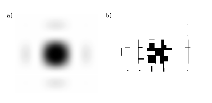
Figure 6: Close-up view of the center of a $(1-{\rm sinc}^{2}x)(1-{\rm sinc}^{2}y)$ mask, a band-limited mask which offers nearly as much search area as a Gaussian spot. (a) Graded version (b) Binary notch filter version.

As a third example, we can combine masks with sampled versions of the uniform mask, $\hat{M}(x)=C$, a constant. Let

$$\hat{M}_{T}(x) = \hat{P}(x)*\Delta x\sum_{n}\delta(x-n\Delta x)$$ (16a)

$$M_{T}(u) = P(u)\sum_{n}\delta(u-n/\Delta x),$$ (16b)

where $\int_{-\infty}^{\infty}\hat{P}(x)\,dx=C$. We can multiply a notch filter mask function by $\hat{M}_{T}(x)$ and obtain another notch filter mask. If we choose $\Delta x=\lambda/D$, and $\hat{P}(x)=(D/\lambda)\Pi(xD/(C\lambda)$, then the new mask will look just like the old one, only painted with black stripes of width $C\lambda/D$, spaced by $\lambda/D$ (Figure 4e), which may run in any direction. Since $\hat{M}_{T}(x)$ diffracts some light outside the Lyot stop, the intensity throughput of this new $\hat{M}_{notch}(x)$ will be reduced—by a factor of $C^{2}$. Combining binary masks and these striped masks may make it possible to design a range of masks which require no supportive substrate.

6 MASK ERRORS

Consider a binary mask like the one shown in Figure 4d, constructed from rectangles of opaque material, of width $\lambda/D$. How sensitive is the coronagraph to errors in the construction of this mask? What if one of these rectangles, in the center of the mask, were accidentally made too short by an amount $h\lambda/D$, where $h<<1$?

A missing rectangle of material—or an extra rectangle of material—would act like a tophat mask, diffracting light around the second pupil plane. A tophat mask is not band-limited and it has a power spectrum that falls off quite slowly with spatial frequency. Therefore it affords only modest cancellation of light in the center of the second pupil plane.

A tophat mask of width $\lambda/D$ and length $h\lambda/D$ produces a diffraction pattern with most of its power in a zone with dimensions $D/\lambda$ by $D/(h\lambda)$. The intensity in this illuminated region is proportional to $h$, but only a fraction $\sim h$ of the illuminated region falls in the center of the Lyot stop. In this portion of the illuminated region which falls in the center of the Lyot stop, the field is roughly uniform, but attenuated by roughly a factor of 2; the intensity is attenuated by a factor of four. Therefore, the final image will acquire an extra image of a point source in the center, with fractional intensity $\sim 0.25h^{2}$.

We can easily tolerate leakages of $\sim 10^{-7.5}$ of the starlight falling in the center of the final image plane. If we are to avoid leaks of greater than this magnitude, we must avoid making the rectangles too short, unless $0.25h^{2}\lesssim 10^{-7.5}$, or $h\lesssim 1/3000$. For a telescope with focal ratio $f$, this tolerance becomes $\lambda f/3000$, or typically $\sim 0.02$  $\mu$m, for $\lambda=1.0$ $\mu$m, $f=60$.

If the error is not in the center of the mask, but in the search area, we can tolerate less leakage intensity, but the light falling on the hole will be diminished in intensity by a similar amount, so the requirement on the size of the hole remains about the same. A hole far from the center, outside the search area, say at $100\lambda/D$, need only have $h<$ a few percent, since the wings of the stellar image that fall on it are typically four or more orders of magnitude weaker in intensity than the core of the stellar image.

The tolerances for binary mask construction given here fall within the reach of standard nanofabrication techniques. Mask defects acquired during a mission may yield to compensation by the active optics a planet-finding coronagraph will require to correct wavefront errors throughout the system. If the hole in the mask described above had dimensions $\lambda/D$ by $\lambda/D$, but had an intensity depth of only $f$, then the hole would cause a fractional stellar leakage of $\sim 0.25f$, as opposed to $\sim 0.25h^{2}$; the shapes of binary masks are much less sensitive to errors than the intensity transmissivities of graded masks.

7 A WORKED EXAMPLE

To further illustrate the use of a notch-filter mask, let us design some notch filter masks for a circular 4m TPF coronagraph (see, e.g., Brown et al. 2002). We will assume a bandpass from $\lambda_{min}=0.66$ $\mu$m to $\lambda_{max}=1.0$ $\mu$m, and a mask construction tolerance of 20 nm. Rather than describing the optics in terms of the dimensionless diffraction scale, $\lambda/D$, we will use the phisical size of the diffraction scale in the focal plane, $\lambda f$, where $f$ is the focal ratio of the telescope. The search problem and the characterization problem call for different specialized image masks, based on different band-limited functions. We will design a search mask—a linear mask rather than a circular mask for the reasons enumerated in Section 5.2.

If we choose a Lyot stop that works at $\lambda_{max}$, the coronagraph will provide equal or better contrast over the whole band. The half power point of the mask, $\theta_{1/2}$, is angle from the optical axis where $\left(\hat{M}_{BL}(\theta_{1/2})\right)^{2}=0.5$; we will choose $\theta_{1/2}=3\lambda_{max}/D$ or 150 mas. This mask will enable us to search for planets as close as $\sim 1$ AU projected distance from a star at 6.5 parsecs. Searching for planets calls for a mask based on a band-limited function with small wings, providing a large search area where the planet image will be relatively unattenuated by the mask. A suitable one with the prescribed half-power point has the form $\hat{M}_{BL}=1-{\rm sinc}^{2}(\pi x\epsilon/(\lambda_{max}f))$ with $\epsilon=0.4$ at $\lambda_{max}$, i.e., $\hat{M}=1-{\rm sinc}^{2}(x/(1.76\lambda_{max}f))$. Since the primary is circular, the shape of the Lyot stop will be the overlap region of two unit circles whose centers are separated by $\epsilon$, as depicted in Figure 4d of Kuchner & Traub (2002).

To estimate the stellar leak due to pointing error and the finite size of the stellar disk, we may re-write Equation 16 in Kuchner & Traub (2002) so that it applies to any linear mask which is roughly quartic inside its half-power point. The fraction of the starlight that leaks through the mask, $L$, is

$$L\approx{{\theta_{\star}^{4}+48(\Delta\theta)^{2}\theta_{\star}^{2}+128(\Delta\theta)^{4}}\over{129\ \theta_{1/2}^{4}}},$$ (17)

where $\theta_{\star}$ is the angular diameter of the star, $\Delta\theta$ is the pointing error in the $x$ direction, and is the half power point of the mask. This equation also applies to nulling interferometers with quartic nulls. However, the half power point of a nulling interferometer’s fringe depends on wavelength.

When the pointing error is somewhat larger than the typical stellar diameter ($\theta_{\star}=1.43$ mas for a G star at 6.5 pc), the pointing error dominates the leak. If the pointing errors, $\Delta\theta$, are distributed in a Gaussian distribution about $\Delta\theta=0$, the mean pointing-error-dominated leak is

$$L\approx 3\left({{\sigma_{\Delta\theta}}\over{\theta_{1/2}}}\right)^{4},\qquad\hbox{for $\sigma_{\Delta\theta}>\theta_{\star}$,}$$ (18)

where $\sigma_{\Delta\theta}$ is the standard deviation of the distribution. If we require a mean leakage of $\sim 3\times 10^{-8}$ of the starlight falling in the center of the final image, the pointing error tolerance becomes $\sigma_{\Delta\theta}\leq\theta_{1/2}/100$, or 1.5 mas.

This leakage due to pointing error can easily be suppressed to the $10^{-10}$ level in the search area given a weakly apodized Lyot stop. For example, an apodization function of the form $\cos{\pi u\lambda/((1-\epsilon/2)D)}$ provides 2.5 orders of magnitude of suppression at $3\lambda/D$. The total throughput of the coronagraph would be $1-\epsilon=0.6$ without the Lyot stop apodization; with the apodization realized as a binary mask, it is 0.358. This apodization is workable, but not optimal; further work on choosing matched pupil and image stops could improve the overall system performance.

Clearly, the leakage due to pointing errors quickly shrinks for planet-finding coronagraphs with larger inner working distances, like the proposed Eclipse mission (Trauger et al., 2002a). For this 2 m class telescope with inner working distance $\sim 300$ mas, a pointing error of $\sigma_{\Delta\theta}=3$ mas suffices to match the above performance. Likewise, if the pointing errors and other low-spatial-frequency errors could be controlled below the levels assumed here, these coronagraph designs could operate at smaller inner working distances.

We will realize the mask as a binary notch filter mask like the one in Figure 4d. In Section 6, we showed that the lengths of the bars in this mask must be accurate to $\lambda f/3000$. Since a hole of a given physical size subtends a larger fraction of $\lambda/D$ at smaller $\lambda$, this tolerance applies at $\lambda_{min}$. In other words, if we can manufacture a mask accurate to 20 nm, we require a focal ratio $f=90$. The strips must have maximum width $<\lambda_{min}f=59.4\mu$m. Explicitly, the mask function would be:

$$\hat{M}_{binary}(x,y)=\left\{\begin{array}[]{ll}0&\mbox{where $|y-n\lambda_{min}f|<{{\lambda_{min}f}\over{2}}\hat{M}_{notch}(x)$}\\ 1&\mbox{elsewhere}.\end{array}\right.$$ (19)

where

$$M_{notch}(x)=\sum_{n}\left(1-{\rm sinc}^{2}\left({{\pi\epsilon(n+\zeta)\lambda_{min}}\over{\lambda_{max}}}\right)\right)\Pi\left({{x}\over{\lambda_{min}f}}-(n+\zeta)\right)-\hat{M}_{0}.$$ (20)

Table 1 shows that our mask has $\hat{M}_{0}=0.0054400$ and $\zeta=0.1017713$.

In the absence of noise, analyzing the data from this coronagraph is trivial. A planet at angle $\theta_{p}$ from the optical axis is simply attenuated by the low spatial frequency components of the notch filter mask, i.e., $\approx\left(1-{\rm sinc}^{2}(\theta_{p}/90{\rm mas})\right)^{2}$. The shape of the PSF is set entirely by the Lyot stop; it is the squared absolute value of Fourier conjugate of the Lyot stop amplitude transmissivity.

8 SIMULATION OF CORONAGRAPH PERFORMANCE

We numerically simulated the performance of this notch-filter coronagraph design by following the Fraunhofer propagation of light through a coronagraph using fast Fourier transforms. Nakajima (1994), Stahl & Sandler (1995) and Sivaramakrishnan et al. (2001) have used this technique to model the performance of ground-based coronagraphs. We simulated the broad-band performance by running the monochromatic simulation 10 times over a range of wavelengths from 0.66 to 1.0 $\mu$m and averaged the output images weighted by the stellar flux, assuming a Rayleigh-Jeans law star and planet. The noise representations remained the same from wavelength to wavelength—scaled appropriately to model pathlength errors rather than phase errors and to reflect the change in the diffraction scale.

We used a 1024 by 1024 grid with resolution $\lambda_{min}/(2D)$. In this representation, errors in the shape of the image mask become variations in the mask amplitude transmissivity. For example, if a bar in the binary mask were too long by $h\lambda/D$, the values of four adjacent elements in the mask amplitude transmissivity matrix would increase by $h$.

We assumed a circular pupil and a Lyot stop with the shape of two overlapping circles as described above multiplied by $\cos{\pi u/((1-\epsilon/2)D))}$. Seen from afar, the contrast between the Earth and the Sun when the Earth is at maximum angular separation is $2\times 10^{-10}$ (Des Marais et al., 2001). We used this contrast level for the planets in our simulation.

Figure 7 shows the intensity in the second pupil plane before (a) and after (b) the Lyot stop for a monochromatic simulation at 1.0 $\mu$m of a system containing a star and a planet at $20\lambda_{max}/D$. The intensity after the Lyot stop has been multiplied by a factor of $10^{9}$. This figure represents a more accurate version of the cartoon in Figure 1. Figure 7a shows how the diffracted light falls within regions of width $\epsilon$ around the left and right edges of the Lyot stop. The notch filter mask adds further illumination to the Lyot stop, farther off axis. Our simulation does not model these artifacts; the Lyot stop blocks them completely. The planet adds a uniform background illumination to the region inside the Lyot stop, though the noise peaks due to wavefront errors and mask errors dominate Figure 7b.

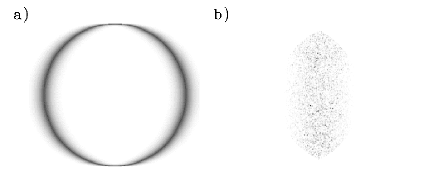
Figure 7: Simulated monochromatic intensity in the Lyot plane for a star and planet system imaged by the coronagraph described in Section 7 a) before the Lyot stop b) after the Lyot stop, amplified by a factor of $10^{9}$.

Figure 8 shows a cut through the final image plane along the $x$-axis. The top panel of the figure shows a plot of $\log\left(1-{\rm sinc}^{2}(\theta_{p}/90{\rm mas})\right)^{2}$. This quantity is the intensity attenuation supplied by the coronagraph, neglecting any modification of the low spatial frequency components of the mask that might occur in the construction of a notch filter representation.

The lower panel of the figure shows the relative surface brightness of several noise contributions to the image, normalized to the peak of what the stellar image would be if the image mask were removed. The dotted curve shows the $10^{-7.5}$ leakage due to pointing error which we prescribed. The form of this curve is simply the Fourier transform of the Lyot stop averaged over the band weighted by the stellar flux. The dash-dot curve shows the consequence of adding white noise to the lengths of the bars with r.m.s. 20 nm. This noise concentrates near the optical axis in the final image plane because it is multiplied by the image of the star that falls on the image mask. This phenomenon suggests that the tolerance of the coronagraph to mask errors can be altered, and possibly improved by manipulating the shape of the entrance pupil.

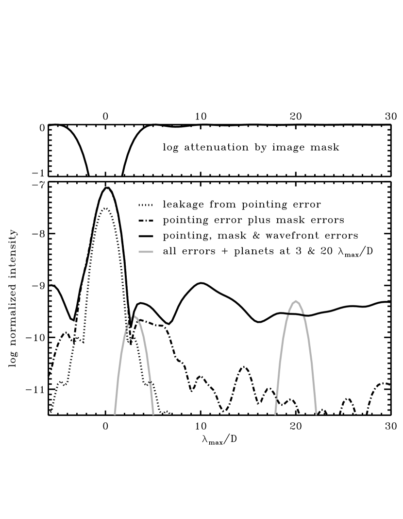
Figure 8: Broadband simulation of images produced by the notch filter coronagraph design described in the text. The dotted curve shows leakage due to pointing error. The dot-dash curve adds errors to the lengths of the mask bars. The solid curve adds amplitude and phase errors to the incoming wavefront. The grey curves show the images of planets with relative flux $2\times 10^{-10}$ at 3 $\lambda_{max}/D$ and 20 $\lambda_{max}/D$. The upper panel shows the attenuation caused by the image mask.

The solid black curve shows the consequence of adding white-noise phase and amplitude errors to the incoming wavefront: fractional amplitude errors of r.m.s. $10^{-3}$ over spatial frequencies corresponding to the search area in the image plane (3–60 $\lambda/D$) and phase errors due to pathlength errors of r.m.s 0.5 Å over these frequencies. A pathlength error of 0.5 Å corresponds to an error in the figure of a mirror of 0.25 Å. Preliminary tests in the High Contrast Imaging Testbed at JPL have demonstrated deformable mirror wavefront control at this level (Trauger et al., 2002a, b). Wavefront errors clearly dominate mask errors and pointing errors, except within a few diffraction widths of the optical axis.

The grey curves show the images of two planets located at $3\lambda_{max}/D$ and $20\lambda_{max}/D$, i.e., 154 mas and 1026 mas—or 0.8 AU and 5.1 AU for a star 5 pc distant. The planet at $3\lambda_{max}/D$ is attenuated by a factor of $0.5$ because it sits at the mask’s half power point. If $Q$ is the contrast between the planet’s peak intensity and the local scattered light background (Brown & Burrows, 1990), the $3\lambda/D$ planet has $Q\approx 0.5$, and the $20\lambda/D$ planet has $Q\approx 1$. Planets with $Q\sim 1$ can easily be detected in a coronagraph using spectral deconvolution techniques, for example, given sufficiently low photon noise (Sparks & Ford, 2002).

9 CONCLUSION

We have illustrated the use of notch filter functions to generate several kinds of image masks which should be relatively easy to manufacture. We showed graded masks whose transmissivities are everywhere greater than zero. We showed binary image masks, which can be cut or shaped from pieces of opaque material. These binary masks can be manufactured to the tolerances necessary for terrestrial planet finding using standard nanofabrication techniques, and can potentially be made self-supporting. Our simulations of the performance of a coronagraph outfitted with a binary notch filter mask suggest that this technique could reveal extrasolar planets similar in brightness to the Earth around nearby stars, given foreseeable improvements in wavefront control on a highly stable space platform.

Binary notch filter masks combine many of the advantages of binary pupil masks (ease of manufacture, achromaticity, robustness) with the advantages of band-limited image masks (large search area, and small inner working distance). Using binary pupil or image masks seems to inevitably require stacking many copies of the same basic aperture shape; Kasdin, Spergel & Littman (2001) used this principle to generate binary pupil masks; we have used it to generate binary image masks. In Kasdin, Spergel & Littman (2001), the high-spatial frequency artifacts of this stacking procedure appear in the image plane directed away from a search sector. In notch filter masks, the high-spatial frequency artifacts are directed into the Lyot stop.

Ultimately, a space telescope for direct optical imaging of extrasolar planets may incorporate more than one diffracted-light management strategy. Having a choice of different techniques available will allow a mission to adapt to changing observing needs as our understanding of high-contrast space telescopes improves and the phenomenology of extrasolar planets unfolds.