The Spiral Structure of the Milky Way,
Cosmic Rays, and Ice Age Epochs on Earth

Abstract

The short term variability of the Galactic cosmic ray flux (CRF) reaching Earth has been previously associated with variations in the global low altitude cloud cover. This CRF variability arises from changes in the solar wind strength. However, cosmic ray variability also arises intrinsically from variable activity of and motion through the Milky Way. Thus, if indeed the CRF climate connection is real, the increased CRF witnessed while crossing the spiral arms could be responsible for a larger global cloud cover and a reduced temperature, thereby facilitating the occurrences of ice ages. This picture has been recently shown to be supported by various data Shaviv, (2002). In particular, the variable CRF recorded in Iron meteorites appears to vary synchronously with the appearance ice ages.

Here we expand upon the original treatment with a more thorough analysis and more supporting evidence. In particular, we discuss the cosmic ray diffusion model which considers the motion of the Galactic spiral arms. We also elaborate on the structure and dynamics of the Milky Way’s spiral arms. In particular, we bring forth new argumentation using HI observations which imply that the galactic spiral arm pattern speed appears to be that which fits the glaciation period and the cosmic-ray flux record extracted from Iron meteorites. In addition, we show that apparent peaks in the star formation rate history, as deduced by several authors, coincides with particularly icy epochs, while the long period of 1 to 2 Gyr before present, during which no glaciations are known to have occurred, coincides with a significant paucity in the past star formation rate.

I Introduction

It has long been known that solar variability is affecting climate on Earth. The first indication for a solar–climate connection can be attributed to William Herschel, (1796), who found that the price of grain in England inversely correlated with the sunspot number. He later suggested that it was due to changes in the solar irradiance Herschel, (1801). The irradiance variability is probably not large enough to explain the climatic variability observed by Herschel, nevertheless, synchronous temperature and solar variations do exist. For example, typical surface temperatures during northern summers were found to differ by $0.5^{\circ}$K to $1.5^{\circ}$K between solar minima and solar maxima Labitzke & van Loon, (1992).

Over the past century, Earth has experienced a gradual, though non-monotonic warming. It is generally believed to be a result of a greenhouse effect by anthropogenic fossil fuel emissions. However, a much better fit is obtained if part of the warming is attributed to a process, or processes, correlated with the solar activity, thus explaining for example, the non-monotonic global temperature change Friis-Christensen & Lassen, (1991); Soon et al., (1996); Beer et al., (2000). Moreover, the part of the climatic variability which is synchronized to the solar activity is larger than could be expected from just the 0.1% typical change in the solar irradiance Beer et al., (2000); Soon et al., (2000). Namely, the variability in the thermal flux itself appears to be insufficient to explain, for example, the global temperature variations observed.

If one goes further back in time, then climatic variability on the time scale centuries, is too correlated with solar activity. Cold episodes in Europe such as the Maunder, Spörer and Wolf Minima clearly correlate with peaks in the ¹⁴C flux, while warm episodes, such as the “medieval warm” period during which Vikings ventured across the Atlantic, correlate with minima in the ¹⁴C flux (e.g., Fastrup et al., (2001)). This flux itself is anti-correlated with the solar activity through the solar wind which more effectively reduces the Galactic cosmic ray flux that reaches Earth (and produces ¹⁴C) while the sun is more active. On a somewhat longer time scale, it was even found that climatic changes in the Yucatán correlate with the solar activity Hodell et al., (2001) (and possibly with the demise of the Maya civilization). While on even longer time scales, it was shown that the monsoonal rainfall in Oman has an impressive correlation with the solar activity, as portrayed by the ¹⁴C production history Neff et al., (2001).

Two possible path ways through which the solar activity could be amplified and affect the climate were suggested. First, solar variations in UV (and beyond) are non-thermal in origin and have a much larger relative variability than that of the total energy output. Thus, any effect in the atmosphere which is sensitive to those wavelengths, will be sensitive to the solar activity. UV is absorbed at the top part of the atmosphere (at typical altitudes of 50 km), and is therefore responsible for the temperature inversion in the Stratosphere. Any change in the UV heating could have effects that propagate downward. In fact, there is evidence that it can be affecting global circulations and therefore also climate at lower altitudes. For example, it could be affecting the latitudinal extent of the Hadley circulation Haigh, (1996).

Another suggested proxy for a solar-climate connection, is through the solar wind modulation of the galactic cosmic ray flux, as first suggested by Ney, (1959). Ney pointed out that cosmic-rays (CRs) are the primary source for ionization in the Troposphere, which in return could be affecting the climate.

First evidence in support was introduced by Tinsley & Deen, (1991) in the form of a correlation between Forbush events and a reduction in the Vorticity Area Index in winter months. Forbush events are marked with a sudden reduction in the CRF and a gradual increase over a typically 10 day period. Similarly, Pudovkin & Veretenenko, (1995) reported a cloud cover decrease (in latitudes of 60N-64N, where it was measured) synchronized with the Forbush decreases. Later, an effect of the Forbush decreases on rainfall has also been claimed Stozhkov & et al., (1995) – an average 30% drop in rainfall in the initial day of a Forbush event (statistically significant to 3$\sigma$) was observed in 47 Forbush events recorded during 36 years in 50 meteorological stations in Brazil. While in Antarctica, Egorova et al., (2000) found that on the first day after a Forbush event, the temperature in Vostok station dramatically increased by an average of 10^∘K, but there was no measurable signal in sync with solar proton events. On the longer time scale of the 11-year solar cycle, an impressive correlation was found between the CRF reaching Earth and the average global low altitude cloud cover Svensmark & Friis-Christensen, (1997); Marsh & Svensmark, (2000).

Although the above results are empirical in nature, there are several reasons to believe why the cosmic-ray route could indeed be responsible for a connection between the solar variability and cloud cover. First, CRs are modulated by the solar activity. On average, the heliosphere filters out 90% of the Galactic CRs (e.g., Perko, (1987)). At solar maximum, this efficiency increases as the solar wind is stronger. Since it takes time for the structure of the heliosphere to propagate outward to the heliopause at 50 to 100 AU and for the CRs to diffuse inward, the CR signal reaching Earth lags behind all the different indices that describe the solar activity (e.g., the sunspot number or the 10.7 cm microwave flux which is known to correlate with the EUV flux). The cloud cover signal is found to lag as well behind the solar activity and it nicely follows the lagging CRF. Second, both a more detailed analysis Marsh & Svensmark, (2000) and an independent study Palle Bago & Butler, (2000) show that the correlation is only with the low altitude cloud cover (LACC). Among the different possible causes which can mediate between the solar variability and climate on Earth, only Galactic CRs can affect directly the lower parts of the atmosphere. It is the Troposphere where the high energy CRs and their showers are stopped, and are responsible for the ionization. EUV variability will affect (and ionize) the atmosphere at higher altitudes ($\gtrsim$ 100 km). As mentioned, thermal heating by Ozone absorption could possibly affect also low altitudes, however, the CRF-cloud cover connection is seen only in low altitude clouds. Solar CRs (which are less energetic than Galactic CRs) are not only stopped at similarly high altitudes, the terrestrial magnetic field also funnels them towards the poles. On the other hand, the LACC-CRF correlation is seen globally.

Last, Tinsley & Deen, (1991) who first found a correlation between Forbush events and a reduction in the Vorticity Area Index in winter months, showed that these events correlate significantly better with the cosmic ray flux than with the UV variations (which generally start a week before the Forbush events). They also suggested that the UV cannot be responsible for this Tropospheric phenomenon since the time scale for the Stratosphere to affect the Troposphere is longer than the Forbush–VAI correlation time scale.

Although the process of how CRs could affect the climate is not yet fully understood, it is very likely that the net ionization of the lower atmosphere (which is known to be governed by the CRF, e.g., Ney, (1959)) plays a major role, as the ionization of the aerosols could be required for the condensation of cloud droplets Dickinson, (1975); Kirkby & Laaksonen, (2000); Harrison, (2000). An experiment is currently being planned to study the possible cosmic-ray flux – cloud-cover connection. It could shed more light and perhaps solidify this connection Fastrup et al., (2001). Moreover, some physical understanding appears to be emerging Yu, (2002). Interestingly, the latter work may explain why the apparent effect is primarily on the lower troposphere and why the global warming of the past century has been more pronounced at the surface than at higher altitudes.

Hence, the evidence shows it to be reasonable that solar activity modulates the cosmic ray flux and that this can subsequently affect the global cloud cover and with it the climate. Assuming this connection to be true, we should expect climatic effects also from intrinsic variations in the CRF reaching the solar system.

With the possible exception of extremely high energies, CRs are believed to originate from supernova (SN) remnants (e.g., Longair, (1994), Berezinskiĭ et al., (1990)). This is also supported with direct observational evidence Duric, (2000). Furthermore, since the predominant types of supernovae in spiral galaxies like our own, are those which originate from the death of massive stars (namely, SNe of types other than Ia), they should predominantly reside in spiral arms, where most massive stars are born and shortly thereafter die Dragicevich et al., (1999). In fact, high contrasts in the non-thermal radio emission are observed between the spiral arms and the disks of external spiral galaxies. Assuming equipartition between the CR energy density and the magnetic field, a CR energy density contrast can be inferred. In some cases, a lower limit of 5 can be placed for this ratio Duric, (2000).

Thus, when the sun passes through the Galactic spiral arms, an increased CRF is expected. If the CRF-LACC connection is real, this will increase the average LACC and reduce the average global temperature. The lower temperatures will then manifest themselves as episodes during which ice ages can occur. Moreover, if the Milky Way as a whole is more active in forming stars, more massive stars will die and produce CRs. We show in this work that both these effects appear to be supported by various data.

Shaviv, (2002) studied this conjecture and found evidence which supports it, thereby strengthening the possibility of a CRF–climate connection. In this work, we elaborate the original treatment by performing a more thorough analysis. We significantly extend the discussion on the dynamics of the spiral pattern of the Milky Way as it is important for determining the reoccurrences of ice age epochs, and introduce a new argument that helps determine the pattern speed. We also introduce more evidence in the form of an apparent correlation between the recorded Milky Way activity (as described by the star formation rate, SFR) and the occurrence of ice age epochs. In particular, it is shown that the lack of glaciation activity on Earth between 1 and 2 Gyr BP (before present) appears to correlate with a dip in the Star formation rate in the same period (at least, as obtained by several but not all authors!). On the more speculative side, since the SFR activity may correlate with the activity in the LMC and with its estimated passages through perigalacticon, ice-ages could be attributed, to some extent, to fly-by’s of the LMC.

It is also interesting to note that other mechanisms have been previously proposed to link the Galactic environment with climate variability on Earth. The first such mechanism was proposed long ago by Hoyle & Lyttleton, (1939) who argued that an encounter of the Solar System with an interstellar cloud might trigger an ice age epoch by increasing the solar luminosity, which produces an over compensating increase in cloudiness. The increased luminosity is a result of the accretion energy released. However, it is currently believed that radiation driving has a positive feedback (e.g., Rind & Overpeck, (1993)), not a strong negative one. Namely, an increase in the solar luminosity will result with an increase of the temperature, not a decrease. Nonetheless, encounters with interstellar clouds could still have a temperature reducing effect if sufficient quantities of dust grains are injected to the upper atmosphere to partially shield the solar radiation Yabushita & Allen, (1985). These events are more likely to occur during spiral arm crossing, since it is there where dense molecular clouds concentrate. However, since they require high density clouds, it seems unlikely that they can explain several $10^{7}$ yr glaciation epochs each spiral crossing.

A second mechanism has to do with the shrinking of the heliosphere. Begelman & Rees, (1976) have shown that while crossing moderately dense ISM clouds with densities of $10^{2}$ to $10^{3}$ cm^-3, the bow shock of the heliosphere will be pushed further in than 1 AU. As a consequence, the slowing down effect that the heliosphere has on Galactic cosmic rays, will cease to work and the flux of Galactic low energy CRs will be significantly increased. On the other hand, the charged particles comprising the solar wind will not reach Earth. Either way, the flux of low energy charged particles reaching Earth could be significantly altered. Although these particles are not known to have a climatic effect at the moment, such an effect cannot be ruled out. Unlike the previous mechanisms, if this route can work, it may require significantly less dense ISM clouds which are more frequent. However, it is still unclear whether a several $10^{7}$ yr long glaciation event can be obtained via this route.

A third mechanism operating mainly during spiral arm crossing is the perturbation of the Oort cloud and injection of comets into the inner solar system. Napier & Clube, (1979) and Alvarez et al., (1980) discussed the effects that grains injected into the atmosphere by cometary bombardment will have on the climate by blocking the solar radiation. Hoyle & Wickramasinghe, (1978) proposed that a cometary disintegration in the vicinity of Earth’s orbit would similarly inject grains into the atmosphere.

One should note that these mechanisms all predict ice-age epochs in synchronization with the spiral arm crossing. This is counter to the model described here in which a phase lag exists.

There were also proposals that related the Galactic year (i.e., the revolution period around the galaxy) to climate on Earth (Steiner & Grillmair, (1973),Williams, (1975), Frakes et al., (1992) and references therein). For example, Williams, (1975) suggested that IAEs on Earth are periodic, and that this rough $\sim 150$ Myr period is half the Galactic year. Williams raised the possibility that this Galactic-climate connection could arise if the disk is tidally warped (e.g., by the LMC), but did not mention a specific mechanism that can translate the warp into a climatic effect. On the other hand, Steiner & Grillmair, (1973) suggested that climatic variability may arise if the solar orbit around the galaxy is eccentric and if, for some unknown physical reason, the solar luminosity is sensitive to the galactic gravitational pull.

Another interesting suggestion for an extraterrestrial trigger for the ice-age epochs, has been made by Dilke & Gough, (1972); (see also Christensen-Dalsgaard et al., (1974)), who showed that the solar core may be unstable to convective instability under the presence of chemical inhomogeneities induced by the nuclear burning. These authors have argued that both the time scales and luminosity variations involved could explain the occurrence of IAEs.

In addition to the extraterrestrial factors, there are also terrestrial factors which are in fact most often claimed by the paleoclimatological community to affect climatic variability on geological time scales. These are the continental geography, sea level, atmospheric composition, and volcanic, tectonic and even biological activity. It is likely that, at least to some extent, many of the aforementioned terrestrial and extraterrestrial factors affect the global climate. Therefore, one of the main questions still open in paleoclimatology is the relevant importance of each climatic factor.

We begin by reviewing the observations and measurements. These include a summary of the glaciation epochs on Earth, the dynamics and star formation history of the Milky Way, and the CRF history as derived from Iron/Nickel meteorites. Some of these results are described here for the first time. We then proceed to describe the model which relates the Galactic environment to climate on Earth though the variability in the CRF, assuming CRs do affect the climate, and follow with the predictions of the model. The model’s backbone is the solution of the problem of CR diffusion while incorporating that the CR sources reside primarily in the spiral arms, and adding the climatic effect that the CRs may have. Then, we continue with a comparison between the proposed theory and observations. We show that an extensive set of tests employing currently available data points to the consistency of the theory.

Table 1: Acronyms

Notation	Definition
BP	Before Present
CR	Cosmic Ray
cR	Co-Rotation
CRF	Cosmic Ray Flux
HI, HII	Atomic, Ionized Hydrogen
IAE	Ice-Age Epoch
LACC	Low Altitude Cloud Cover
LMC	Large Magellanic Cloud
MW	Milky Way
SFR	Star Formation Rate
SN	Supernova

II The Observations and Measurements

We begin by reviewing several seemingly unrelated topics: The evidence for climatic variability on Earth on a time scale of $10^{7}-10^{9}$ yr, as portrayed by the occurrence of ice ages, the dynamics of the Milky Way with its spiral structure in particular, as well as the data on CR exposure ages from Fe/Ni meteorites. Some of the observational conclusions are essentially quoted “as is” while several results are obtained by analyzing previously published data.

II.1 Earth’s glaciation history

During the course of Earth’s history, the climate has been variable on all time scales ranging from years to eons. Since clear geological signatures are left from periods when Earth was cold enough to have extensive glaciations, studying the occurrence of ice-ages is a good method to quantify long term climatic variability, though it is not the only way (for example, we could have studied the occurrence of “evaporates” left during warm periods). We therefore choose to look at the occurrence of ice-ages.

Before we continue, we should point out that ice-ages on Earth appear on two time scales. Over ${\mathcal{O}}(10^{4})$ yr, ice ages come and go. However, epochs during which ice ages can appear or epochs during which ice ages can be altogether absent, exist on time scales of ${\mathcal{O}}(10^{7})$ yr. In the rest of our discussion, the term ice-age epoch (IAE) will correspond to these long epochs. Today, we are in the midst of a long IAE, though specifically in a mid-glaciation period between ${\mathcal{O}}(10^{4})$ yr long ice-ages.

Extensive summaries describing the IAEs experienced by Earth are found in Crowell, (1999) and in Frakes et al., (1992). These mostly rely on geological evidence of ice ages for the occurrence of glaciations, but not only. The nature of the glaciations in the Phanerozoic ($0-545$ Myr BP) are to a large extent well understood. Partially it is because more recent data is more readily available and partially because dating layers with fossils is easier. Moreover, the analysis of Veizer et al., (2000) who measured the tropical sea surface temperatures over the Phanerozoic serves as an independent analysis from those studying the occurrence of glaciations. As can be seen in figure 10 and table 2, the different analyses are quite consistent with each other.

The Neo-Proterozoic (1000 - 550 Myr BP) was probably an intrinsically cooler period in Earth’s history, and glaciation was more abundant than in the Phanerozoic. However, two epochs stand out as particularly more glaciated. These are Crowell, (1999) the Marinoan and Varangian Glaciations (545 - 585, 590 - 640 Myr BP) and the Sturtian Glaciations (700 - 750 Myr BP). In the former, the extent of glaciations was particularly impressive, with evidence of low latitude sea level glaciations, which triggered ideas such as the ‘Snowball Earth’ Hoffman et al., (1995). A third, earlier epoch around ca. 900 Myrs BP is still very questionable, with some less firm indications pointing to it ($\sim 940$ Myr according to Williams, (1975), and ca. $900$ Myr according to others, Hambrey & Harland, (1985), Crowell, (1999)). To be conservative, we will not take this epoch in our analysis (though it does nicely correlate with a spiral arm crossing if it existed). Before 1000 Myr BP, there are no indications for any glaciations, expect for periods around 2.2 - 2.4 Gyr BP and 2.9-3.0 Gyr BP. The lack of glaciations could be attributed to a changed solar orbit within the Galaxy. However, since the probability for the solar system to abruptly change its Galactic orbit is very small, this change which occurred at 1 Gyr BP, is more likely to be attributed to intrinsic variations in the climate—for example, due to a slow reduction in greenhouse gases, or to variations in the MW’s average SN rate.

The paleoclimatological data of Crowell, (1999), Frakes et al., (1992) and Veizer et al., (2000) is summarized in table 2, together with our adopted age for the mid point of the ice-age epochs and its error. Panel C,D and E in fig. 10 depict a graphical summary of the appearance of glaciations in the past 1 Gyr.

As a big word of caution, one should note that the glaciation data does not come without its caveats. For example, unlike Frakes et al., (1992), Crowell believes that the data is insufficient to claim periodicity in the occurrence of IAEs. See §V.1 and fig. 10 for a detailed summary of the caveats.

Table 2: Ice Age Epochs from geological records (in Myr BP)

Midpoint of IAEs1			Adopted Age	Spiral Arm	Total
Crowell	Frakes	Veizer	and Error2	Error3	Error
$\lesssim 15$	$\lesssim 28$	$\sim 30$	$20\pm 10$	11	15
$\sim 155$	$\sim 144$	$\sim 180$	$160\pm 10$	11	15
$\sim 325$	$\sim 293$	$\sim 310$	$310\pm 20$	12	24
$\sim 450$	$\sim 440$	$\sim 450$	$446\pm 10$	13	17
$\sim 595$	$\sim 588$	–	$592\pm 15$	14	21
$\sim 730$	$\sim 765$	–	$747\pm 20$	15	25
$\sim 900$	$\sim 940$	–	$920\pm 20$	16	26

¹ Crowell, (1999) is the mid point of the epochs with glacial activity. Frakes et al., (1992) is the midpoint of the “ice house” periods, while Veizer et al., (2000) is the time with the coldest tropical sea temperatures, for which evidence exists in the past 550 Myr.

² The adopted age is the average of Crowell, (1999), Frakes et al., (1992) and Veizer et al., (2000), except for the present IAE. Since it is ongoing, its midpoint is likely to be more recent. The adopted error is a rough estimate. It considers that the error in recent IAEs is smaller and that short IAEs are much easier to pin point in time.

³ The “Spiral Arm Error” is the error arising from the epicyclic motion of the solar system. That is, it arises from the non circular motion that it can have around the galaxy. It effectively introduces a ‘jitter’ in the predicted location of the spiral arms (see appendix B).

II.2 Spiral Structure and Dynamics of the Milky Way

The exact pattern speed of the spiral arms of Milky Way and in fact the spiral structure itself, is still considered an open question. This is primarily because of our internal vantage point inside the Milky Way. Since these will soon be required, we review the current status and analyze the data available.

II.2.1 Milky Way Spiral Structure

A review of the different measurements for the spiral structure, and in particular the number of arms is given by Vallée, (1995, 2002) and by Elmegreen, (1998). Vallee concluded that 4 arms are more favorable than two. Elmgreen concluded that 4 arms appear to govern the outer part of the Milky Way, while the inner part is much more complicated. The problem in the determination of the actual spiral structure is that distances to objects are either not known accurately enough or they do not trace the spiral arms unambiguously, if particular objects are used (for example, HII regions, OB stars or Cepheids). If a smooth component is analyzed instead (such as the distribution of molecular gas) then the distance, which is inferred from velocity measurements and the Milky Way rotation curve, is a multi-valued function of the gas velocity within the solar circle. It is then hard to disentangle the spiral structure from the observed $l-v$ (longitude velocity) maps. The main exception to the above is the HI (or similar) measurements of gas outside the solar circle. Since HI traces the spiral arms nicely, and since outside the solar circle no velocity-distance ambiguities exist, the spiral structure can be “read off” the $l-v$ maps straight forwardly. The result is a clear 4-arm spiral structure Blitz et al., (1983); Dame et al., (2001). We therefore assume that at the solar galactocentric radius and beyond, the spiral structure of the Milky Way is that of 4 arms. This does not imply that further inside the Galaxy the same 4-arm structure exists. In fact, we shall show that there is a good reason for the two structures to be different (which could explain why until now the picture was confusing).

II.2.2 The Spiral Arm Pattern Speed – Previous Results

Even less agreed upon and more confusing are the results for the pattern speed $\Omega_{p}$ of the spiral arms in the Milky Way. For the sake of completeness, we first review previous determinations of $\Omega_{p}$. We will afterwards continue with a new analysis which was previously applied to other galaxies but never to our own.

A survey of the literature reveals that quite a few different analyses were performed to measure the Galactic spiral arm pattern speed. Some methods are local in the sense that they look at local age gradients of young objects, such as OB stars or open clusters. These are presumably methods which rely on the least number of (Galactic) assumptions. For example, they should detect the correct pattern speed irrespective of whether the spiral arm is a density wave or just a star formation shock wave (without a density wave associated with it), or irrespective of whether the MW has 2 or 4 spiral arms. Unfortunately, these methods tend to be inaccurate because of local “dispersions” and inaccuracies in age determinations.

A second type of methods looks at the birth place of objects not as young as before. These include, for example, the birth place of open clusters with a typical age of a few $10^{8}$ yr. This can in principle help place more accurate constraints on the pattern speed. However, unlike the previous methods, it requires a model for the spiral arms including their number, their amplitude and pattern speed, all of which should be fitted for. In reality, one often assumes both that the number of arms and their amplitude are given within the context of the density wave theory. Then, several different guesses for $\Omega_{p}$ are guessed and the best fit is chosen.

A third type of methods relies on fitting the observed velocities of stars to a spiral density wave, and in particular the non-circular residue obtained after their circular component is removed. The advantage of this type of a measurement is that it does not rely on age determinations at all, since it relies on the “instantaneous” configuration. However, the residual kinematics are sensitive to the rotation curve chosen as well as to the spiral wave parameters.

A fourth type of methods relies upon the identification of resonance features expected to arise from the spiral density wave theory. For example, Gordon, (1978) identifies the observed discontinuity in CO emission at about 4 kpc with the inner Lindblad resonance.

A summary of the various determinations of $\Omega_{p}$ in the literature is found in table 3. The main result apparent from the table is that most of the values obtained for $\Omega_{p}$ cluster within two ranges ($\Omega_{\odot}-\Omega_{p}\sim 9-13.5$ km sec^-1 kpc^-1and $\Omega_{\odot}-\Omega_{p}\sim 2.5-5$ km sec^-1 kpc^-1), with a third range being either a tail for the second or a real “cluster” of results (for which $\Omega_{\odot}-\Omega_{p}\sim($-$1)-($-$4)$ km sec^-1 kpc^-1). Interestingly, the division between the clusters is not a function of the method used. For example, Palous et al., (1977) have shown that two equally acceptable values are obtained from the same analysis. Clearly, the results in the literature are still not converged, but possible values and unaccepted ranges can be inferred.

II.2.3 Pattern Speed from HI Observations

As previously mentioned, relying on particular objects to identify the spiral structure has the disadvantage of distance inaccuracies and that these objects do not always trace the spiral arms nicely enough. One the other hand, mapping of various gas components has the disadvantage that the velocity-distance ambiguities can complicate the analysis significantly. Therefore, analyzing gas at Galactic radii larger than the sun ($R\gtrsim R_{\odot}$) has a clear advantage, as it avoids the above ambiguities and uncertainties.

Blitz et al., (1983) found that a four armed spiral structure in HI extends all the way to $R_{\rm HI,out}\approx 2R_{\odot}$. (Specifically, they found $R_{\rm HI,out}=20$ kpc when taking a rotation curve in which $R_{\odot}=10$ kpc and $v_{\odot}=200~{}{\rm km/s}$. For more up to date rotation curves, the value of $R_{\rm HI,out}$ is lower but still roughly twice our galactocentric radius). Moreover, more upto date HI maps, as traced by CO reveal the spiral arms outside the solar galactocentric radius even more clearly Dame et al., (2001), thus reinforcing the results of Blitz et al., (1983). This observation on the external radius of the galactic spiral arms can be proven useful to constrain the pattern speed, if this 4-arm structure is a spiral density wave.

According to spiral density wave theory, 4-armed spiral density waves can only exist within the inner and outer 4:1 Lindblad resonances (e.g., Binney & Tremaine, (1988)). Otherwise, the waves become evanescent. The inner and outer 4:1 Lindblad resonances, $R_{I4:1}$ and $R_{O4:1}$, are defined through:

$$\Omega_{\odot}(R_{I4:1})-{\kappa(R_{I4:1})\over 4}=\Omega_{p}=\Omega_{\odot}(R_{O4:1})+{\kappa(R_{O4:1})\over 4},$$ (1)

where $\Omega(R)$ and $\kappa(R)$ are respectively the rotational frequency and the epicyclic frequency at radius $R$. Therefore, the constraint $R_{\rm HI,out}\leq R_{O4:1}$ that the arms should terminate before or at the outer Lindblad resonance can be rewritten as

$$\Omega_{p}\leq\Omega_{\odot}(R_{\rm HI,out})+{\kappa(R_{\rm HI,out})\over 4}.$$ (2)

To obtain the numerical value of the r.h.s., we need to know the rotation curve of the Milky Way. We use the summary given by Olling & Merrifield, (1998), which includes the range of currently acceptable rotation curves for which $R_{\odot}$ ranges from 7.2 to 8.5 kpc. For each rotation curve, we recalculate the outer extent of the HI arms which the Blitz et al., (1983) result corresponds to. We then calculate the location of the resonances and their constraint on the pattern speed (eq. 2). This is portrayed in figure 1. The results are given in table 4. They imply that:

$$\Omega_{p} \lesssim 16.9\pm 2.5~{}\mathrm{km~{}sec^{-1}~{}kpc^{-1}}$$ (3)

$$\Omega_{\odot}-\Omega_{p} \gtrsim 9.1\pm 2.4~{}\mathrm{km~{}sec^{-1}~{}kpc^{-1}}.$$

Again, it should be stressed that the results assume that the spiral arms are a density wave. However, if they are, then the limit is robust since 4 spiral arms are clearly observed to extend to about twice the solar galactocentric radius. Spiral density wave theory has thus far been the most successful theory to describe spiral features in external galaxies Binney & Tremaine, (1988), therefore, it is only reasonable that it describes the spiral arms in our galaxy as well. Moreover, in alternative theories in which the spiral arms are for example shocks formed from stellar formation, one would not expect to see spiral arms beyond the stellar disk, which is “truncated” several kpc inwards from $R_{\rm HI,out}$ Robin et al., (1992); Ruphy et al., (1996).

This last point, combined with the fact that HI is seen beyond the outer extent of the arms (to $R\approx 3R_{\odot}$) implies that their outer limit is probably the actual 4:1 resonance. In other words, the relations given by eq. 3 are probably not just limits but actual equalities. The reason is that there is otherwise no other physical reason to explain why the arms abruptly end where they are observed to do so. (They do not end because of lack of HI nor does the stellar population has anything to do with it).

Further theoretical argumentation can strengthen the last point made. The co-rotation (cR) point, has often been linked to spiral arm brightness changes in external galaxies. The reason is that the spiral arm shocks are important at triggering star formation. However, near co-rotation, the shocks are very weak. This is often seen in external galaxies as an “edge” to the disk, external to which the surface brightness is much lower (e.g., Elmegreen, (1998)). If the 4-arm pattern has the aforementioned pattern speed, then the cR radius can be predicted. This radius (relative to $R_{\odot}$) is given in the seventh column of table 4. We find that $R_{cR}-R_{\odot}=6.5\pm 1.5$ kpc. For comparison, observations of stellar distributions show that there is a sharp cutoff of stars at $R_{cR}-R_{\odot}=5.5$ to $6$ kpc according to Robin et al., (1992) or, $R_{cR}-R_{\odot}=6.5\pm 2$ kpc according to Ruphy et al., (1996). These numbers are also in agreement with a sharp truncation of the CO mass surface density at $R_{cR}-R_{\odot}=5\pm 0.5$ kpc Heyer et al., (1998). Namely, observations are consistent with the cR radius predicted using the calculated pattern speed, provided that the sharp cut-off is related to the CR radius. This is also in direct agreement of Ivanov, (1983) who finds a co-rotation radius at 11-14 kpc for $R_{\odot}=8$ kpc.

The last argument for why the constraint given by eq. 3 should be considered an equality and not a limit is the following. If $\Omega_{p}$ is significantly lower than the limit given by eq. 3, then the inner extent of the 4-arms, as constrained by the inner 4:1 Lindblad resonance, should be outside the solar circle. However, according to the Blitz et al., (1983) and Dame et al., (2001) data, the 4-arms extend inward at least to the solar circle. On the other hand, table 3 shows that the 4 arms cannot extend much further in. Thus, not only should eq. 3 be considered a rough equality, the spiral structure inside the solar circle has to have different kinematics than the structure of the external 4-arms. This could explain the large confusion in the spiral structure and pattern speeds. This could also explain why several authors find that the solar system is located near co-rotation. If we are near CR, then it would be the co-rotation radius of the inner spiral structure. Nevertheless, this point is still far from having a satisfactory explanation. See §V.1 for more details.

Considering now that the first range of results in table 3 appears to be consistent with the density wave theory and the observations of HI outside the solar circle, we average the results in this range to get a better estimate for the pattern speed. We find $\Omega_{\odot}-\Omega_{p}=11.1\pm 1$ km sec^-1 kpc^-1. This translates into a spiral crossing period of $134\pm 25$ Myr on average (taking into account the results of appendix B).

Table 3: The observational determinations of the Milky Way spiral arm pattern speed.

First	$\Omega_{\odot}$	$\Omega_{p}$	$\Omega_{\odot}-\Omega_{p}$	Method / Notes
Author	(km/s)/kpc	(km/s)/kpc	(km/s)/kpc
Yuan (1969a)	25	$\sim 13.5^{1}$	$\sim 11.5$	Arm dynamics fit to Lin & Shu
Yuan (1969b)	25	$\sim 13.5$	$\sim 11.5$	Migration of young stars
Gordon (1978)	25	$11.5\pm 1.5$	$13.5\pm 1.5$	CO discontinuity at 4 kpc is ILR
Palous (1977)	25	$\sim 13.5$	$\sim 11.5$	Cluster birth place
Grivnev (1983)	25	12-16	9-13	Cepheid birth place
Ivanov (1983)	27.5	16-20	7.5-11.5	Cluster age gradients
Comerón (1991)	25.9	$16\pm 5$	$10\pm 5$	Kinematics of young stars
Creze (1973)	$\sim 24.5$	$\sim 22$	$2.5\pm 1.5$	Kinematics of young stars
Palous (1977)	25	$\sim 20$	$\sim 5$	Cluster birth place
Nelson (1977)	25	$\sim 20$	$\sim 5$	Spiral Shocks profile & 21cm line
Mishurov (1979)	25	$23.6\pm 3.6$	$1.4\pm 3.6$	Kinematics of Giants & Cepheids
Grivnev (1981)	25	$21-23$	2-4	Kinematics of HII regions
Efremov (1983)	25	$18-25$	0-7	Cepheid age gradients
Amaral (1997)	23.3	$21\pm 1$	$2.3\pm 1$	Cluster birth place
Avedisova (1989)	25.9	$26.8\pm 2$	$-1\pm 2$	Age gradient in Sag-Car
Mishurov (1999)	$26\pm 2$	$28.1\pm 2$	$-2\pm 3$	Cepheids kinematics
Fernández (2001)	25.9	$30\pm 7$	$-4\pm 7$	OB Kinematics
Here (HI)	$26.5\pm 1.2$	$16.9\pm 2.5$	$9.1\pm 2.4$	$r_{out}\approx r_{O4:1}$ of 4 HI arms2
Here (CRF var.)	–	–	$10.5\pm 0.8_{stat}\pm 1.5_{sys^{3}}$	CRF variability in Fe meteorites
Here (ice-ages)	–	–	$10.4\pm 0.35_{stat}\pm 1.5_{sys^{3}}$	Fit to ice-age occurrence4

¹ Some results have no quoted error, but they should typically be $\pm 1$ km sec^-1 kpc^-1. For example, Palous et al (1977) checked specific pattern speeds: 11, 13.5, 15, 17.5, 20, 21.5 and found that only 13.5 and 20 agree with cluster birth places.

² In principle, the 4 HI arms can terminate at $r_{\mathrm{HI,out}}<r_{\mathrm{O4:1}}$ (in which case $\Omega_{p}$ can be smaller and $\Omega_{\odot}-\Omega_{p}$ larger than the quoted numbers), however, as explained in the text, there is evidence pointing to $r_{\rm HI,out}$ actually being $r_{O4:1}$.

³ The origin of the systematic error is from possible diffusion of the solar system (both radially and along its azimuthal trajectory), relative to an unperturbed orbit. This is explained in appendix B. The values include the expected correction ($0.54\pm 1.5$ km sec^-1 kpc^-1) due to the solar metallicity anomaly.

⁴ The agreement between the bottom three results form the basis for the spiral arms – ice age epochs connection.

Figure 1: The dynamical frequencies of the Milky Way relevant to its spiral structure, plotted as a function of galactocentric radius. Using a typical rotation curve (taken from Olling & Merrifield, (1998)), one can calculate $\Omega$ and the epicyclic frequency $\kappa$. Spiral density wave theory states that a four arm spiral cannot exist for $\Omega_{p}>\Omega+\kappa/4$. Since a four arm spiral is observed in HI to extend out to $r_{\rm HI,out}\approx 2R_{\odot}$, an upper limit on $\Omega_{p}$ can be placed. This $\Omega_{p}$ implies that the inner edge of the arm structure should be located roughly at our galactocentric radius with only two arms possibly penetrating further in (e.g. Amaral & Lepine, (1997)), if an $m=2$ component exists with the same $\Omega_{p}$.

Table 4: Implications of the 4-arm HI¹ data using spiral density wave theory and a possible range for the Milky Way rotation curve.

$R_{\odot}$	$v_{\odot}$	$\Omega_{\odot}$	$R_{\rm HI,out}$	$R_{\mathrm{in}}$	$R_{\mathrm{in}}$ - $R_{\odot}$	$R_{\mathrm{cR}}-R_{\odot}$	$\Omega_{\mathrm{p,max}}$	$\Omega_{\odot}-\Omega_{\mathrm{p,max}}$	$\Omega_{\mathrm{b,min}}^{(2)}$
$\mathrm{kpc}$	$\mathrm{km\over s}$	$\mathrm{km\over s~{}kpc}$	$\mathrm{kpc}$	$\mathrm{kpc}$	$\mathrm{kpc}$	$\mathrm{kpc}$	$\mathrm{km\over s~{}kpc}$	$\mathrm{km\over s~{}kpc}$	$\mathrm{km\over s~{}kpc}$
7.1	184	25.92	16.2	8.3	1.2	5.1	14.39	11.52	30.1
7.1	200	28.17	15.7	7.1	0.0	5.0	17.64	10.59	29.5
8.5	220	25.88	18.7	6.4	-2.1	7.7	18.21	7.7	27.4
8.5	240	28.24	18.3	7.4	-1.1	7.9	19.35	6.7	27.2
$7.8$	$212$	$26.5$	$17.2$	$7.3$	-0.5	$6.5$	$16.9$	$9.1$	$28.6$
$\pm 0.7$	$\pm 30$	$\pm 1.2$	$\pm 1.5$	$\pm 1$	$\pm 1.7$	$\pm 1.5$	$\pm 2.5$	$\pm 2.4$	$\pm 1.5$

¹ HI data is from Blitz et al., (1983). Rotation curves are from Olling & Merrifield, (1998).

² The MW appears to have a bar which ends at 3 to 4.5 kpc. Since bars typically end between the I4:1 resonance and cR, a lower limit on the bar’s pattern speed $\Omega_{b}$, can be placed (assuming the bar ends at 4.5 kpc and coinciding with I4:1 resonance). Since $\Omega_{\rm p,max}<\Omega_{\rm b,min}$, at least two different pattern speeds exist in the MW.

II.3 Star Formation History of the Milky Way

In general, the intrinsic flux of cosmic rays reaching the outskirts of the solar system (and which we will soon require) is proportional to the star formation rate (SFR) in the solar system’s vicinity. Although there is a lag of several million years between the birth and death of the massive stars which are ultimately responsible for cosmic ray acceleration, this lag is small when compared with the relevant time scales at question. In the “short term”, i.e., on time scales of $10^{8}$ yrs or less, this “Lagrangian” SFR should record passages in the Galactic spiral arms. On longer time scales, of order $10^{9}$ yrs or longer, mixing is efficient enough to homogenize the azimuthal distribution in the Galaxy. In other words, the SFR on long time scales, as recorded in nearby stars, should record long term changes in the Milky Way SFR activity. This may arise for example, from a merger with a satellite or nearby passages of one.

Scalo, (1987), using the mass distribution of nearby stars, found SFR peaks at 0.3 Gyr and 2 Gyr before present (BP). Barry, (1988) and a more elaborate and recent analysis by Rocha-Pinto et al., (2000a) (see also references therein), measured the SFR activity of the Milky Way using chromospheric ages of late type dwarfs. They found a dip between 1 and 2 Gyrs and a maximum at 2-2.5 Gyrs BP. As a word of caution, there are a few authors who find a SFR which in contradiction to the above. More detail can be found in the caveats section §V.1.

These SFR peaks, if real, should also manifest themselves in peaks in the cluster formation rate. To check this hypothesis, the validity of which could strengthen the idea that the SFR was not constant, we plot a histogram of the ages of nearby open clusters. The data used is the catalog of Loktin et al., (1994). From the histogram apparent in figure 2, two peaks are evident. One, which is statistically significant, coincides with the 0.3 Gyr SFR event. The second peak at 0.6 Gyr, could be there, but it is not statistically significant. Thus, we can confirm the 300 Myrs event. Note that this cluster histogram is not corrected for many systematic errors, such as the finite life time of the clusters or finite volume effects. As a result, the secular trend in it is more likely to be purely artificial. The same cannot be said about the non-monotonic behavior of the peaks.

One source for a variable SFR in both the LMC and MW could be the gravitational tides exerted during LMC perigalactica. According to the calculations of the perigalacticon passages, these should have occurred within the intervals: 0.2-0.5 Gyr BP, 1.6-2.6 Gyr BP and 3.4-5.3 Gyr BP (with shorter passage intervals obtained by Gardiner et al., (1994), and the longer ones by Lin et al., (1995); the further back, the larger the discrepancy). Interestingly, the 0.3 Myr and 2 Gyr BP SFR events are clearly located in the middle of the possible LMC perigalacticon.

Apparently, the MW activity is also correlated with SFR activity in the LMC. At 2 Gyr BP, it appears that there was a significant increase in the SFR in the LMC. Photometric studies of the HR diagram by Gallagher et al., (1996) show a prominent increase in the SFR somewhat more than 2 Gyrs before present. An increase in the SFR 2-3 Gyrs before present was also found by Vallenari et al., (1996). Dopita et al., (1997) analyzed planetary nebulae and found that the LMC metallicity increased by a factor of 2 about 2 Gyrs BP, and Westerlund, (1990) has shown that between 0.7 and 2 Gyrs BP, the LMC had a below average SFR.

Figure 2: The history of the Star Formation Rate (SFR). The squares with error bars are the SFR calculated using chromospheric ages of nearby stars Rocha-Pinto et al., (2000a). These data are corrected for different selection biases and are binned into 0.4 Gyr bins. The line and hatched region describe a 1-2-1 average of the histogram of the ages of nearby open clusters using the Loktin et al., (1994) catalog, and the expected 1-$\sigma$ error bars. These data are not corrected for selection effects (namely, the upward trend with time is a selection effect, favorably selecting younger clusters). Since the clusters in the catalog are spread to cover two nearby spiral arms, the signal arising from the passage of spiral arms is smeared, such that the graph depicts a more global SFR activity (i.e., in our Galactic ‘quadrant’). On longer time scales (1.5 Gyrs and more), the Galactic stirring is efficient enough for the data to reflect the SFR in the whole disk. The dashed histogram underneath is the same as the histogram above it, though only with clusters having a better age determination ($w>1.0$, as defined in Loktin et al., (1994)). There is a clear minimum in the SFR between 1 and 2 Gyr BP, and there are two prominent peaks around 0.3 and 2.2 Gyr BP. Interestingly, the LMC perigalacticon should have occurred sometime between 0.2 and 0.5 Gyr BP in the last passage, and between 1.6 and 2.6 Gyr BP in the previous passage. This might explain the peaks in activity seen. This is corroborated with evidence of a very high SFR in the LMC about 2 Gyrs BP and a dip at 0.7 - 2 Gyr BP. Also depicted are the periods during which glaciations were seen on Earth: The late Archean (3 Gyr) and mid-Proterozoic (2.2-2.4 Gyr BP) which correlate with the previous LMC perigalacticon passage Gardiner et al., (1994), Lin et al., (1995), and the consequent SFR peak in the MW and LMC. The lack of glaciations in the interval 1 - 2 Gyr before present correlates with a clear minimum in activity in the MW (and LMC). Also, the particularly long Carboniferous-Permian glaciation, correlates with with the SFR peak at 300 Myr BP and the last LMC perigalacticon. The late Neo-Proterozoic ice ages correlate with a less clear SFR peak around 500-900 Myr BP.

II.4 Cosmic Ray Flux history from Iron Meteorites

When meteorites break off from their parent bodies, their newly formed surfaces are suddenly exposed to cosmic rays, which interact with the meteorites through spallation. The spallation products can be stable nucleotides, which accumulate over time, or they can be unstable. In the latter case, their number increases but eventually reaches saturation on a time scale similar to their half life. The ratio therefore between the stable and unstable nucleotides can be used to calculate the integrated CRF that the meteorite was exposed to from the time of break up to its burning in the atmosphere. Generally, it is assumed that the CRF is constant, in which case the integrated flux correspond to a given age through a linear relation Singer, (1954); Lavielle et al., (1999).

A twist on the above, however, takes place in measurements employing the ${}^{41}{\rm K}/^{40}{\rm K}$ ratio. Since the unstable isotope in the pair has a half life slightly longer than 1 Gyr, it does not reach saturation. By comparing the age of meteorites using this method to methods which employ unstable isotopes with a short half life (decay time $\lesssim$ a few Myr), it was found that the CRF in the past several Myr has been higher by about 30% than its average over 150 to 700 Myr BP Lavielle et al., (1999). In principle, if the measurements were accurate enough, the slight inconsistencies between the two types of methods, as a function of time, could have been translated into a CRF history. However, a simulation shows that except for the flux variation over the past several Myrs, this method becomes unfeasible. This can be seen in figure 3.

To extract the CRF, another method should be used. If we look at figure 3, we see that points on the graph which are separated by equal real-time intervals, tend to bunch near the minima of the CRF signal, when plotted as a function of potassium exposure age. This statistical clustering effect can be used to extract the CRF, if a large sample of dated meteorites is used.

As previously mentioned, CR exposure dating assumes that the flux had been constant in history. However, if it is not, the assumed CR exposure time will not progress linearly with the real time. During epochs in which the CRF is low, large intervals of time will elapse with only a small increase in apparent CR exposure age. As a result, all the meteorites that broke off their parent body during this interval, will cluster together. On the other hand, epochs with a higher CRF will have the opposite effect. The CR exposure clock will tick faster than the real clock such that meteorites that broke off during this period will have a wide range of exposure ages. Thus, the number of meteorites per “apparent” unit time will be lower in this case.

We use the data of Voshage & Feldmann, (1979) and Voshage et al., (1983). Together, we have a sample of 80 meteorites which were ${}^{41}{\rm K}/^{40}{\rm K}$ dated. In principle, we could also use meteorites which where exposure dated using unstable isotopes other than ${}^{40}{\rm K}$, however, this will introduce more complications. Because the other isotopes used for exposure dating have a relatively short life time, the relation between the real age and the exposure age is sensitive to the ratio between the recent CRF (over a few Myr) and the average over the past 1 Gyr. This is not the case with ${}^{40}{\rm K}$. The second advantage of using the ${}^{40}{\rm K}$ data is that it encompasses more meteorites, which is important for the statistics. In the future, a more extensive and detailed analysis should clearly consider the additional data and the complications that it introduces.

Since we are assuming that meteoritic surfaces are formed homogeneously in time, we should be careful not to be fooled from the effects that real clustering can have. To minimize this, we removed all meteorites which have the same classification and are separated by less than 100 Myr. These are then replaced by their average.

The result is a data set containing 50 meteorites. We then plot a histogram of the CR exposure age of the meteorites in figure 4. Immediately apparent from the figure is a periodicity of $143\pm 10$ Myr. Moreover, if we plot a scatter plot of the error as a function of age, we see a tendency to have a higher error in points falling in the gaps between the clusters. This can be expected if the clustering signal is real since points with a smaller error will more easily avoid the gaps, thereby generating a bias. This consistency check helps assure we are looking at a real signal. If the apparent periodic signal would have been a random fluctuation, there would have been no reason to have larger errors in the random gaps, except from yet another unrelated random fluctuation.

Next, we fold that data over the apparent period to overcome the systematic error arising from the slowly changing selection effects. Once we fold the data over the period, we find an even clearer signal. We perform a Kolmogorov-Smirnov test on the folded data and find that the probability for a smooth distribution to generate a signal as non uniform as the one obtained, is only 1.2% in a random set of realizations. Therefore, it in unlikely that the meteoritic distribution was generated from a purely random process. Conversely, however, the K-S test can only say that the distribution is consistent with a periodic signal.

Furthermore, we can also predict the distribution using the diffusion model described in §III.2. In the graphs we take the nominal case of $D=10^{28}~{}{\rm cm}^{2}/{\rm sec}$ and $l_{H}=2$ kpc (as will be shown in §III), and find that the distribution obtained fits the predicted one. In particular, the phase where the obtained distribution peaks agrees with observations. This implies that the significance is of order 1:500 (instead of 1:80) to have a random signal accidentally produce the apparently periodic signal and in addition has the correct phase.

The agreement between the amplitude predicted and observed is less significant. The reason is that by changing the diffusion model parameters, the contrast can be changed (as is apparent in table 5).

Another point to consider is the error in the CR ages. Although errors were quoted with the exposure age data, their values are quite ad hoc Voshage, (1967). By comparing the Potassium age to ages determined using other methods, it is evident that the quoted errors over estimate the actual statistical error. The scatter in the difference between the Potassium age and the age in other methods is typically 30 Myr. This implies that the actual statistical error in the Potassium age determinations is at most 30 Myrs, though it should be smaller since some of the error should be attributable to the second age determination. Since the error will have the tendency to smear the distribution, the obtained contrast between the minimum and maximum flux is only a lower limit.

To summarize, the Iron/Nickel meteoritic exposure age distribution appears to have a periodicity of $143\pm 10$ Myr. The signal is not likely to arise from a random process, and it also has the correct phase to be explained by spiral arm crossings. The CRF contrast obtained (in the folded distribution) is $\left<\max(\Phi)/\min(\Phi)\right>\gtrsim 3$. In addition it has been previously obtained that the flux today is higher by about 30% than the average flux over the past billion years. Both these constraints should be satisfied by any model for the CR diffusion in the galaxy.

Figure 3: Theoretical comparison between different exposure ages of Iron meteorites and their real age. Plotted as a function of the Potassium exposure age ($a_{\rm K}$) are the real age ($a_{\rm real}$, in solid line) and a non-Potassium exposure age ($a_{\rm Be}$, such as using ${}^{10}{\rm B}/^{21}{\rm Ne}$ dating, with a dashed line), and $a_{\rm K}$ (using a dotted line, with a unit slope). Also plotted are the predicted CRF relative to the present flux ($\Phi/\Phi_{0}$) as a function of $a_{\rm real}$, and $\rho_{t}$–the (unnormalized) expected number of Potassium exposure ages per unit time, as a function of $a_{\mathrm{K}}$. A histogram of $a_{\mathrm{K}}$ should be proportional to $\rho_{t}$. The horizontal and vertical dotted lines describe how $\rho_{t}$ is related to the relation between $a_{\rm real}$ and $a_{\mathrm{K}}$—equally spaced intervals in real time are translated into variable intervals in $a_{K}$, thereby forming clusters or gaps in $a_{\mathrm{K}}$. The graph of $a_{\rm Be}$ vs. $a_{\rm K}$ demonstrates that comparing the different exposure ages is useful to extract recent flux changes (which determine the slope of the graph). On the other hand, the graph of $\rho_{t}$ demonstrates that a histogram of $a_{K}$ is useful to extract the cyclic variations in the CRF, but not for secular or recent ones.

Figure 4: Histogram of the Iron meteorites’ exposure ages. The lowest panel marks the $a_{\rm K}$ ages on the x-axis and the quoted age error on the y-axis. Even by eye, the ages appear to cluster periodically. The second panel is a 1:2:1 averaged histogram of meteorites with a quoted age determination error smaller than 100 Myr, showing more clearly the clustering peaks. Altogether, there are 6 peaks from 210 to 930 Myr BP. The period that best fits the data is $143\pm 10$ Myr. The third panel is similar to the first one, with the exception that the data is folded over the periodicity found. It therefore emphasizes the periodicity. A Kolmogorov-Smirnov test shows that a homogeneous distribution could generate such a non-homogeneous distribution in only 1.2% of a sample of random realization. Namely, the signal appears to be real. This is further supported with the behavior of the exposure age errors, which supply an additional consistency check. If the distribution is intrinsically inhomogeneous, the points that fill in the gaps should on average have a larger measurement error (as it is ‘easier’ for these points to wonder into those gaps accidentally, thus forming a bias). This effect is portrayed by the dotted line in the panel, which plots the average error as a function of phase—as expected, the points within the trough have a larger error on average.

III The Model

We now proceed with a detailed description for how the dynamics of the Milky Way is expected to affect climate on Earth. We begin with the large astronomical scale and work our way down the chain of physical links. Namely, we begin with a model for the CR behavior in the Galaxy and its relation to the spiral arms in particular. This will enable us to quantitatively predict the expected variability in the CRF. We then proceed to estimate the effects that this variability will have on cloud cover and the effects that the latter will have on the average global temperature.

III.1 Dynamics of the Milky Way

The key ingredient which will be shown to be the “driving” force behind climatic variability on the long $\sim 10^{8}$ yr time scale, is our motion around the Galaxy. Variability arises because the Milky Way, like other spiral galaxies does not have cylindrical symmetry—it is broken with the presence of spiral arms.

The basic parameters that determine this variability are the solar system’s distance from the center of the Galaxy $R_{\odot}$, its Galactic angular velocity $\Omega_{\odot}$, the angular pattern speed of the spiral arms $\Omega_{p}$, and their number $m$. Given these parameters, a spiral crossing is expected to occur on average every time interval of

$$\Delta t_{\rm spiral}\approx{2\pi\over m|\Omega_{\odot}-\Omega_{p}|}.$$ (4)

For typical values (as obtained in §II), a spiral crossing is expected to occur every ${\mathcal{O}}(10^{8}~{}{\rm yrs})$. The next step, is to understand and predict the CRF variability that will arise from these spiral arm crossing events.

III.2 A Diffusion Model for the long term Cosmic Ray Variability

Qualitative theoretical and observational arguments were used to show that the CR density should be concentrated in the Galactic spiral arms. The next step is to construct an actual model with which we can quantitatively estimate the variability expected as the solar system orbits the Galaxy.

The simplest picture for describing the CR content of the galaxy is the “leaky box”, which assumes no spatial structure in the CR distribution “inside” the galaxy, and that the probability for a CR particle to remain inside the galaxy falls exponentially in time, with a time constant $\tau_{e,lb}$. Namely, the general equation describing the density of a specie $i$ is given by (e.g., Berezinskiĭ et al., (1990)):

$${dN_{i}\over dt} = Q_{i}+\sum_{j>i}{P_{ij}\over\tau_{j}}N_{j}-N_{i}\left({1\over\tau_{e,lb}}+{1\over\tau_{s}}+{1\over\tau_{r}}\right)$$ (5)

$$\equiv {\tilde{Q}}_{i}-{N_{i}\over\tau_{i,\mathrm{eff}}}.$$

$\tau_{\mathrm{i,eff}}$ is the effective time scale for decay for specie $i$ which includes loss from the galaxy, spallation destruction and radioactive decay. ${\tilde{Q}}_{i}$ is the sum of all sources for specie $i$ which include its actual formation $Q_{i}$ and the result of spallation of more massive species $j$ (which has a spallation time scale of $\tau_{j}$ and a branching ratio $P_{ij}$ to form specie $i$).

Eq. 5 can be generalized to the case when spatial and energy homogeneity are not assumed. One then obtains:

$${\partial N_{i}\over\partial t}=D\nabla^{2}N_{i}+{\partial\over\partial E}\left[b(E)N_{i}\right]-{N_{i}\over\tau_{i}}+{\tilde{Q}}_{i}.$$ (6)

The $b(E)$ term corresponds to the slowing down of the CR rays. For the energies at interest, we can safely neglect it as its time scale is very long. Here, $\tau_{i}$ is the effective time scale for spallation or radioactive decay. The leaky box $\tau_{e,lb}$ should not be included explicitly in $\tau_{i}$, since proper losses from the galaxy are implicitly included through losses from the boundary conditions.

The simplest of such models are 1D diffusion models which assume a slab geometry for the galaxy. More complicated models take more careful consideration of the structure of the galaxy by including the radial behavior, making them 2D in nature. However, these models do not consider that the sources reside primarily in the spiral arms (cf. Berezinskiĭ et al., (1990)). We therefore construct a simple model in which the spirals are taken into account.

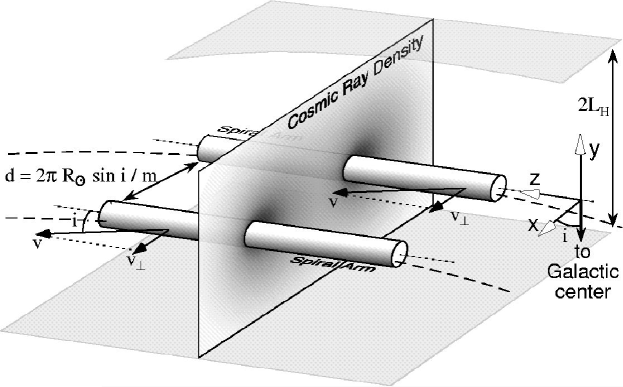
Figure 5: The components of the diffusion model constructed to estimate the Cosmic Ray flux variation. We assume for simplicity that the CR sources reside in gaussian cross-sectioned spiral arms and that these are cylinders to first approximation. This is permissible since the pitch angle $i$ of the spirals is small.

A cartoon describing the geometry of the problem solved in given in figure 5. In particular, we assume the following assumptions:

1. The Galaxy is a slab of width $2l_{H}$. Within it, a diffusion coefficient $D$ exists for the cosmic rays at the relevant energy $\sim 10~{}{\rm GeV}$. Out of this region, the diffusivity is much larger such that CRs can effectively escape in a negligible time. This can be described with a boundary condition of the form $\Phi_{CR}=0$ at $z=\pm l_{H}$.

2. The CR sources are located in cylinders with a Gaussian cross-section. This deserves some explanation. First, in the Taylor & Cordes, (1993) model for the free electron distribution (which we use), the best fit to the free electron density is obtained with $\sigma_{x}=h_{z}=300~{}\mathrm{pc}$ where $\sigma_{x}$ is the width of the horizontal Gaussian distribution $\propto\exp(-x^{2}/2\sigma_{x}^{2})$ and $h_{z}$ is the width in the function ${\rm sech}^{2}(z/h_{z})$ which was used for the fit. Namely, we simplify the problem by assuming that the vertical distribution is Gaussian as well, but with the same length scale as in Taylor & Cordes, (1993). Second, the assumption that the spiral arms are straight cylinders is permissible, since the spirals are tightly wound: $i\approx 12^{\circ}$ with $i$ being their pitch angle). That is, on the typical distance separating the arms, the radius of curvature of the arms is much larger. The actual distance taken between them is:

   $$d_{ij}=\Delta\phi_{ij}R_{\odot}\sin i,$$ (7)

   where $\Delta\phi_{ij}$ is the angular separation between arms $i$ and $j$ according to the Taylor and Cordes model. The distribution of the free electrons and of the cosmic ray sources should be similar since the massive stars that undergo supernovae and produce CRs are also the stars that ionize the interstellar medium. More careful consideration later on will actually show that there is a small but noticeable temporal lag between the two.

3. The arms are moving at a speed $v_{\perp}=(\Omega_{p}-\Omega_{\odot})R_{\odot}\sin i$ in a direction perpendicular to their axes. This is permissible since under the above geometry, there is symmetry along the arms’ axes, implying that their motion along their axis has no effect on the CR distribution.

We should consider that we currently reside in the “Orion Arm”, which is only a spur or armlet Georgelin & Georgelin, (1976). Although it is not part of the global structure of our galaxy, we are required to take it into account in the calculation of the recent CRF variation. As a consequence, we should expect because of it to witness a cosmic ray flux that is higher than predicted in the minimal four arm model. Since the density of HII regions in this spur is roughly half of the density in the real nearby arms Georgelin & Georgelin, (1976), we assume it to have half the typical CR sources as the main arms.

Since the lifetime of these “spurs” is expected to be of order the spiral arm crossing period (e.g., Feitzinger & Schwerdtfeger, (1982)), they are not expected to repeat themselves after a whole revolution, nor can we predict other possible “transient” spiral armlets that we might have crossed in the past.

The free parameters therefore left in the model are the diffusion coefficient $D$, the halo half width $l_{H}$, and the pattern speed of the spiral arms $\Omega_{p}$. Typical values obtained in diffusion models for the CRs yield $D\sim 10^{28}{\rm~{}cm^{2}/s}$ and $R_{h}\sim 2\mathrm{~{}kpc}$ Berezinskiĭ et al., (1990); Webber & Soutoul, (1998); Lisenfeld et al., (1996).

We assume that the heliospheric structure does not vary over intervals of a few 100 Myr. Even if it does, since the cosmic ray energies in question are large ($\gtrsim 10$ GeV/nucleon), the heliosphere will not affect the CRF by more than $\sim 10\%$ Perko, (1987). Thus, the change in the flux reaching the solar system is also the change in the flux reaching the Earth.

We first solve for the CR flux itself and later solve explicitly for the Be nuclei which are used to date the “age” of the CRs. For the CR flux, we can neglect the effect of spallation. We also neglect the ionization energy losses. We therefore solve a simplified version of eq. 6:

$${\partial\Phi\over\partial t}=D\nabla^{2}\Phi+{S}.$$ (8)

$S$ is the source distribution given by the moving cylindrical arms:

$$S=\sum_{i}A_{i}\exp\left\{-{(x-x_{i,0}-v_{\perp}t)^{2}\over 2\sigma_{x}^{2}}-{z^{2}\over 2\sigma_{z}^{2}}\right\},$$ (9)

where $A_{i}$ and $\sigma_{x,z}$ are the amplitude of arm $i$ (with a global normalization that is yet to be determined) and the horizontal and vertical width of the arms. $x_{i,0}=\phi_{i,0}R_{\odot}\sin i$ is the current day “location” of these arms in the model geometry in which the spirals are straightened. $\phi_{i,0}$ is the galactocentric angle of the arms at the solar galactocentric radius. These numbers, together with $\Delta\phi_{i}$ are taken from Taylor & Cordes, (1993).

To solve the diffusion problem, we take full advantage of the fact that eq. 8 is linear. The problem is time dependent. Hence, we begin by writing the solution in the form:

$$\Phi({\bf x},t)=\int_{-\infty}^{t}dt^{\prime}\varphi({\bf x}-(x_{i,0}+v_{\perp}t){\hat{\bf x}},t;t^{\prime}),$$ (10)

where $\varphi({\bf x},t;t^{\prime})$ is the solution (at ${\bf x},t$) for the diffusion for the cosmic rays that where emitted at time $t^{\prime}$. This function can be written as:

$$\varphi({\bf x},t;t^{\prime})=\sum_{i}\varphi_{i}({\bf x}-(x_{i,0}+v_{\perp}t){\hat{\bf x}},t;t^{\prime},i)$$ (11)

namely, as a contribution from each separate arm. We can then further use the method of mirror images which ensures that on the boundaries at $\pm l_{H}$ the CR flux will vanish. We do so by writing:

$$\varphi_{i}({\bf x},t;t^{\prime},i)=\sum_{m=-\infty,\infty}\varphi_{i,0}({\bf x}-2ml_{h}{\bf\hat{z}},t;t^{\prime},i)(-1)^{m}$$ (12)

where $\phi_{i,0}$ is the flux at ${\bf x}$ and $t$ of the CRs emitted at $t^{\prime}$ by arm $i$ assuming it is centered at $x^{\prime}=0$ at $t^{\prime}$, when no boundaries are present. This has the form:

$$\varphi_{i,0}({\bf x}-2ml_{h}{\bf\hat{z}},t;t^{\prime},i)=$$

$$= A_{i}\int_{-\infty}^{\infty}\hskip-4.0ptdx^{\prime}dz^{\prime}{\exp\left(-{(x-x^{\prime})^{2}+(z-z^{\prime})^{2}\over 4D\Delta t}\right)\over 4\pi D\Delta t}{\exp\left(-{{x^{\prime}}^{2}\over 2\sigma_{x}^{2}}-{{z^{\prime}}^{2}\over 2\sigma_{z}^{2}}\right)\over 2\pi\sigma_{x}\sigma_{z}}$$ (13)

$$= A_{i}{\exp\left(-{x^{2}\over 2(2D\Delta t+\sigma_{x}^{2})}-{z^{2}\over 2(2D\Delta t+\sigma_{z}^{2})}\right)\over 2\pi\sqrt{2D\Delta t+\sigma_{x}^{2}}\sqrt{2D\Delta t+\sigma_{z}^{2}}}.$$

with $\Delta t\equiv t-t^{\prime}$. From equation 12, we have that on the $z=0$ plane (i.e., for $|z|\ll l_{H}\sim{\mathcal{O}}(1~{}kpc)$)

$$\varphi_{i}(x,z=0,t;t^{\prime},i)=$$ (14)

$$= A_{i}{\exp\left(-{x^{2}\over 2(2D\Delta t+\sigma_{x}^{2})}\right)\vartheta_{4}\left(0,\exp\left[-2l_{H}^{2}/(2D\Delta t+\sigma_{z}^{2})\right]\right)\over 2\pi\sqrt{2D\Delta t+\sigma_{x}^{2}}\sqrt{2D\Delta t+\sigma_{z}^{2}}}$$

$$\approx {\exp\left(-{x^{2}\over 2(2D\Delta t+\sigma_{x}^{2})}\right)\over\sqrt{2\pi(2D\Delta t+\sigma_{x}^{2})}}{1\over l_{H}}\left[\left(l_{H}^{2}\over 2\pi(2D\Delta t+\sigma_{z}^{2})\right)^{1.8}+1\right]$$

$$\times\exp\left[-{2.4674\over l_{H}^{2}}\left(D\Delta t+{\sigma_{z}^{2}\over 2}\right)\right]$$

where $\vartheta_{4}$ is the Elliptic Theta function of the fourth kind and the approximation is accurate to $\pm 3\%$. We find that the effect of the boundary condition is to introduce an exponential decay. This shows that the diffusion model with boundaries is very similar to the leaky box model, with a decay time constant of $\tau_{e}=l_{H}^{2}/(2.47D)$. In fact, for $t-t^{\prime}+\sigma_{z}^{2}/(2D)\gtrsim\tau_{e}/3$ the error between a simple exponential fit and the Elliptic theta function is less than 10%.

If we go back steps 10 and 11, we finally obtain:

$$\hskip-9.0pt\Phi(x,z=0,t) = \sum_{i}A_{i}\int_{-\infty}^{t}dt^{\prime}{\exp\left(-{\left(x-(x_{i,0}+v_{\perp}t)\right)^{2}\over 2(2D(t-t^{\prime})+\sigma_{x}^{2})}\right)\over 2\pi\sqrt{2D(t-t^{\prime})+\sigma_{x}^{2}}}$$

$$\times {\vartheta_{4}\left(0,\exp\left[-2l_{H}^{2}/(2D(t-t^{\prime})+\sigma_{z}^{2})\right]\right)\over\sqrt{2D(t-t^{\prime})+\sigma_{z}^{2}}}.$$

The global normalization of the amplitudes $A_{i}$ is determined by calculating the time average $\left<F_{CR}(x,y=0,t)\right>$ which from record in Iron Meteorites should be 28% less than todays flux Lavielle et al., (1999).

III.2.1 CR lag after spiral arm crossing

An interesting point worth particular note is that the CR distribution is expected to lag behind the spiral arm passages. Two separate physical mechanisms are responsible for such a lag.

CR distribution skewness: Because the CR distribution is skewed towards later times, the CRF is higher at a given time after the spiral arm crossing than before the crossing. This is because the CRs diffuse in the interstellar medium, but the spiral arms which are their source are moving, thus leaving behind them a wake of slowly diffusing CRs. Before an arm reaches the region of a given star, the CR density is low since no CRs were recently injected into that region and the sole flux is of CRs that manage to diffuse to the region from large distances. After the spiral arm crosses the region, the CR density is larger since locally there was a recent injection of new CRs which only slowly disperse.

This lag is intrinsic to the the diffusion model and therefore need not be considered separately. It can be seen in fig. 7, in the skewed distributions seen around each spiral arm crossing. Although the peak flux is lagged by only a small amount due to this effect, the skewness implies that the mid-point of epochs that are defined by the CRF being larger than a threshold value, will be lagged. Table 5 shows that this lag can range from 6 to 19 Myrs, depending on the model (while considering only those that fit the observed ${}^{10}\mathrm{Be/Be}$ and CRF variations) and assuming a threshold that will soon be shown to correspond to ice-age epochs.

SN-HII lag: A second delay between the CRF distribution and the midpoint of the spiral arm passage arises because the definition of the spiral arm used does not have to coincide with the actual CR source distribution, which are SN remnants. In our case, the spiral arms location is defined through the free electron distribution as fitted for by Taylor & Cordes, (1993) using the pulsar dispersion data. The free electron density is primarily affected by luminous OB stars that are blue enough to ionize the interstellar medium. Therefore, the midpoint of the free electron distribution will occur around half the life span of the stars which dominate the ionization, namely, a few Myr since it is dominated by the most massive O stars that form. SNe on the other hand, occur at the end of the life of stars which can have lower masses and therefore have longer life spans than the stars that dominate the ionization. Since the least massive stars that undergo SN are about 8$M_{\odot}$ and have a life span of typically 35 Myr, the average SN occurs at typically half this life span (as a result of the contribution of more massive stars).

To better quantify this lag, we use the program of Leitherer et al., (1999) which calculates various properties of a starburst population. In particular, it can calculate the flux of ionizing photons and the SN rate, both of which we require. We use standard parameters for a starburst Leitherer et al., (1999). Namely, $10^{6}M_{\odot}$ are formed at $t=0$ with a Salpeter IMF (i.e., a slope of -2.35), with a lower cutoff of 1 $M_{\odot}$, an upper cutoff of 100 $M_{\odot}$ and a minimum mass of 8 $M_{\odot}$ needed to trigger a SN explosion. It also calculates the wind loss using a theoretical estimate and using the Kurucz-Schmutz spectra. The results are depicted in figure 6. It shows that the average ionizing radiation is emitted at 2.0 Myr after the starburst, while an average SN takes place at 17.4 Myr after the starburst, giving an average delay of 15.4 Myr. The single most important parameter to which this lag is sensitive to is the lower cutoff mass needed to form a SN. On the other extreme, the global normalization does not affect the lag at all, implying that the total mass of stars formed and the lower cutoff for star formation are both unimportant. The figure also shows a more realistic distribution obtained not for an instantaneous starburst, but one that has a Gaussian distribution with $\sigma_{t}=16.5$ Myr. This gives a Gaussian distribution for the ionizing radiation expected for an arm of width $\sigma_{arm}\approx 300$ kpc (for the pattern speed that will later be shown to agree with the various data). This width is the value obtained by the Taylor & Cordes, (1993) model. The result for the SN rate in this case, is similar to a Gaussian distribution with a new variance of $\sigma_{t}\approx 20$ Myr.

If we wish to incorporate these two results to the CR diffusion, we need to correct the following:

1. The spiral arm locations, as defined by the CR sources, are lagged by 15.4 Myr after the spiral arms as defined through HII.

2. The width of the CR distribution is spatially (or temporally) larger by a factor of 19.5/16.4 = 1.20 than the one obtained from the Taylor & Cordes, (1993) model.

Figure 6: The ionizing radiation flux and SN rate as a function of time for a starburst of $10^{6}M_{\odot}$ at time $t=0$, assuming standard parameters Leitherer et al., (1999). The heavy weight lines describe the total H ionizing radiation flux (dashed) and the SN rate (solid). Since SNe are dominated by less massive stars than those responsible for the ionization, and since SNe occur only at the end of the stellar life, the SNe distribution is lagging behind the ionization distribution by 15.4 Myr (the average ionizing radiation is emitted at 2.0 Myr after the starburst, while the average SN explodes 17.4 Myr after it). The light weight lines are the same as before only the instantaneous starburst is replaced with a Gaussian distribution with $\sigma=16.5$ Myr, which reproduces the HII arms seen by Taylor and Cordes. The lag remains the same, but the distribution for the SNR widens to 20 Myr.

III.2.2 Effects of inter-arm SNe

We have assumed thus far that SNe occur only within the spiral arms. There are however two SN sources outside the spiral arms. These are from infrequent ‘field’ OB stars and from SNe of type Ia, of which the progenitors are not massive stars.

“Field” SNe: Most star formation in spiral galaxies occurs inside the spiral arms, as a result of gas being shock excited by spiral arm passages. Nevertheless, some star formation occurs outside the arms. To estimate the fraction of the latter, we look at two types of observations – the distribution of giant HII regions and of O stars. HII regions are formed from the ionizing radiation of the massive stars that later explode as SNe. According to Evans, (1991), about 15% of these regions reside in the inter-spiral regions. This can give an upper estimate for the inter-arm SNe rate (of types others than Ia), since 15% is the number fraction of regions—it is not weighed by the actual number of OB stars in each complex (which is expected to be higher in the arms, where HII clouds are larger on average). A lower limit for the SNe rate in the inter-arm regions would be given by the fraction of O stars that reside in the inter-arm regions. O stars are more massive of the stars that undergo SNe explosions; they are therefore expected to be more concentrated in the spiral arms. According to the data in Lynds, (1980), about 20 of the 400 or so nearby O stars reside outside the nearby spiral arms, or 5%. A reasonable estimate for the field SNe rate would therefore be 10% of the spiral arm rate. It is interesting to note that the discrepancy between SNe rate estimates from historical records and from observations in external galaxies has been attributed to SN being distributed mainly in the spirals of the galaxy Dragicevich et al., (1999).

SNe Type Ia: SNe Type Ia are believed not to originate from the core collapse of a single massive star. As a result, they can be found everywhere in the disk, not limited to within the spiral arms. For the same reason, they are also found in Elliptical galaxies. Their fractional rate in Spiral galaxies, depends on the spiral type and to a larger extent, the analysis used to derive the numbers. Typical numbers obtained are 23% for Sab and Sb’s, and 9% for Sbc-Sd Tammann et al., (1994), or, 8%-23% for Sab and Sb’s, and 10%-19% for Sbc-Sd van den Bergh & McClure, (1994). i.e., A typical number expected for the Milky way is 15%.

Both the above inter-arm SN sources add up to typically 25% of the rate in arms. (And it is unlikely to be more than 35% or less than 15% of the rate in the arms). Does this ratio correspond to an additional constant in the CR source that is 25% of the CRs generated in the arms? It would if CR acceleration efficiency was the same in spiral arms and outside of them. However, theoretical argumentation points to an efficiency proportional to the ambient density $n$ Bell, (1978). There are also consistent observations to corroborate this. Radio emission from SNRs in M33, which is presumably from CRs synchrotron emission, is seen only in SNRs located in apparently denser environments Duric, (2000). This would imply that the inter-arm SNe will accelerate less efficiently the CRs, by the typical density ratio between arm and inter-arm regions.

Thus, the average inter-arm SN to arm SN CR generation ratio, is expected to be:

$$\mathcal{S}\equiv{\left<\Phi_{\rm inter-arm}\right>\over\left<\Phi_{\rm arm}\right>}\approx{\left<\rho_{\rm inter-arm}\right>\over\left<\rho_{\rm arm}\right>}{\left(f_{\mathrm{Ia}}+f_{\mathrm{II,Ib}}f_{\mathrm{field~{}OBs}}\right)\over f_{\mathrm{II,Ib}}(1-f_{\mathrm{field~{}OBs)}}},$$ (16)

where $f_{\mathrm{Ia}}$ is the fraction of SN Ia’s, $f_{\mathrm{II,Ib}}=1-f_{\mathrm{Ia}}$ is the fraction of SNe of other type, and $f_{\mathrm{field~{}OBs}}$ is the fraction of massive stars that form outside of the Galactic spiral arms. According to Lo et al., (1987), the typical arm/inter-arm density contrast in $H_{2}$, is at least 3 but can be as high as 15. While it is typically 6 in $H\alpha$ Lees & Lo, (1990). Thus, for the nominal values for the different fractions and a density contrast of 6, we obtain that $\mathcal{S}\sim 5\%$. For the extreme values for the different fractions and density contrast, it can range from 1% to 15%. This is the “background” constant CRF that one has to add to the spiral arm source of CRs. That is, when calculating the flux, we have to add a constant to it:

$$\Phi_{\mathrm{total}}=\Phi_{\mathrm{arm}}+\mathcal{S}\left<\Phi_{\mathrm{arm}}\right>.$$ (17)

III.2.3 Results for the CR diffusion

After incorporating the effect of the inter-arm SNe and the lag generated by the SN delay, results for the CRF can be obtained. Given $D$, $v$ ($\leftrightarrow\Omega_{p}$) and $l_{H}$, we can calculate the variability in the CR flux. We can also calculate the “age” of the CRs as will be measured by the ${}^{10}{\rm Be}/^{9}{\rm Be}$ ratio. This is described in Appendix A. Sample variations of the CRF and the Be age as a function of time are given in figure 7.

Figure 7: The cosmic-ray flux variability and age as a function of time for $D=10^{28}{\rm~{}cm^{2}/s}$ and $l_{H}=2$ kpc. The solid line is the cosmic-ray flux, the dashed line is the age of the cosmic rays as measured using the Be isotope ratio. The shaded regions at the bottom depict the location, relative amplitude (i.e., it is not normalized) and width of the spiral arms as defined through the free electron density in the Taylor and Cordes (1993) model. The peaks in the flux are lagging behind the spiral arm crosses due to the SN-HII lag. Moreover, the flux distribution is skewed towards later times.

Table 5: Results for the spiral arm CR diffusion model¹

$D_{28}$	$l_{H}$	$\tau_{e}$	$\Phi_{\mathrm{min}}/$	$\Phi_{\mathrm{max}}/$	$\Phi_{\mathrm{max}}/$	$\left<\Phi\right>/$	Mid Point	$a_{0}$	$(a)_{\mathrm{min}}$	$(a)_{\mathrm{max}}$	$\Delta T$
	kpc	Myr	$\Phi_{0}$	$\Phi_{0}$	$(\Phi)_{\mathrm{min}}$	$\Phi_{0}$	Lag [Myr]	[Myr]	[Myr]	[Myr]	[∘K]
0.32	0.50	10.54	0.05	2.33	44.66	0.65	5.32	6.54	4.75	16.89	32.40
0.10	0.50	33.74	0.07	1.96	27.92	0.62	12.06	24.98	13.59	75.74	26.95
0.03	0.50	105.43	0.13	1.68	12.93	0.66	17.19	40.39	17.61	114.69	22.13
0.01	0.50	337.38	0.17	1.60	9.18	0.71	18.17	41.45	14.73	128.06	20.29
1.00	1.00	13.49	0.22	1.76	7.87	0.73	6.64	9.14	7.19	15.02	21.75
0.32	1.00	42.17	0.23	1.58	6.97	0.70	8.62	30.90	22.23	58.88	19.25
0.10	1.00	134.95	0.22	1.43	6.62	0.69	17.37	49.52	29.77	101.00	17.21
0.03	1.00	421.73	0.21	1.48	6.99	0.72	18.09	50.10	22.91	121.00	17.98
3.20	2.00	16.87	0.56	1.27	2.26	0.82	5.95	12.08	11.59	15.20	10.02
1.00	2.00	53.98	0.54	1.23	2.28	0.80	9.20	38.12	33.80	50.68	9.74
0.32	2.00	168.69	0.43	1.22	2.86	0.76	10.71	56.75	45.18	83.92	11.22
0.10	2.00	539.81	0.29	1.26	4.36	0.73	18.80	59.73	37.74	107.39	13.79
10.00	4.00	21.59	0.90	1.16	1.29	0.97	3.70	15.76	15.76	17.95	3.66
3.20	4.00	67.48	0.84	1.12	1.32	0.92	5.54	42.52	42.45	48.92	3.85
1.00	4.00	215.92	0.69	1.08	1.56	0.84	9.28	60.86	57.54	72.78	5.46
0.32	4.00	674.76	0.49	1.13	2.30	0.78	11.79	65.62	54.16	90.75	9.03

Note: ¹ The results summarized in this table are a subset of the all the models calculated (and appearing in fig. 8).

Figure 8: Models which fit the observational constraints. The free parameters in the diffusion model are the Diffusion coefficient $D$ and the half width of the Galactic halo (relevant for the diffusion). “O” denote models which fulfill the constraint on the ratio between the maximum flux and the minimum flux (once folded over the 143 Myr period). “V” denotes models which satisfy the constraint on the ratio between today’s flux and the average over the past billion years. “A” denote models which satisfy the “age” constraint of the CRs, as measured by the ${}^{10}{\rm B}/{\rm B}$ ratio.

III.2.4 Constraints on the diffusion model

The primary constraint used to place limits on CR diffusion models is the ${}^{10}\mathrm{Be}/\mathrm{Be}$ ratio observed. This ratio depends on the typical duration the CRs spend between their formation and their detection in the solar system, i.e., on the CR’s typical age. This is because Be isotopes are basically formed as spallation products. ⁹Be is stable and therefore accumulates with time. On the other hand, ¹⁰Be has a decay time scale of several Myr. It therefore saturates.

In appendix A, the survival fraction of ${}^{10}\mathrm{Be}/\mathrm{Be}$ is calculated using the spiral arm diffusion model. This ratio can then be translated to an effective confinement age that a “leaky box” model is required to have for it to yield the same Be ratio. The results are summarized in table 5. This results should be compared with the measured ${}^{10}\mathrm{Be}/\mathrm{Be}$ ratio. The various observed values for this number once translated to an effective CR age in the leaky box model yield $24^{+12}_{-6}$ Myr (see appendix A). Namely, values ranging from 18 to 36 Myr are reasonable, and should be recovered by any consistent diffusion model, including the present one.

Unlike other diffusion models, the spiral arm diffusion model can have more constraints placed on it using the observed CRF variability. Since previous models are all in steady state, they cannot under any condition, satisfy these constraints.

Constraints on the CRF variability can be placed using CR exposure ages of Iron meteorites. Comparison between ages measured using ${}^{41}\mathrm{K}/^{40}\mathrm{K}$ dating in which the unstable isotope ${}^{41}\mathrm{K}$ has a very long half life (1.27 Gyr) and other measurements employing a “short lived” isotope (decay time $\lesssim$ few Myr), have been consistently inconsistent. The only viable explanation being that the CRF in the past several Myrs has been roughly 30% higher than the average over the past billion years Hampel & Schaeffer, (1979); Schaeffer et al., (1981); Lavielle et al., (1999). We take $\Phi_{0}/\left<\Phi\right>=0.7\pm 0.1$. An even more interesting constraint can be placed using the actual CRF variation, as extracted from the distribution of CR exposure ages (see §II.4). This gives $\max(\Phi)/\min(\Phi)\gtrsim 3$ . For various reasons given in §II.4, an upper limit cannot be placed.

Table 5 and fig. 8 summarize the results. Values consistent with the different constraints on the effective leaky box age, with the ratio between the flux today and the average flux, and with the minimum to maximum flux contrast are emphasized in the figure. Since models are required to satisfy all three observed constraints, we can place limits on the diffusion coefficient $D$ and the halo half width $l_{H}$. These are $10^{26}\mathrm{~{}cm}^{2}\mathrm{/s}\lesssim D\lesssim 10^{28}\mathrm{~{}cm}^{2}\mathrm{/s}$ and $0.5\mathrm{~{}kpc}\lesssim l_{H}\lesssim 2\mathrm{~{}kpc}$ (with the values being correlated).

If we return back to table 5, we see that the models satisfying the constraints have a maximum variation of the CRF of $\delta\equiv(\max\Phi-\min\Phi)/\Phi_{\mathrm{today}}\sim 1.0$ to $1.9$ and a lag $a_{0}$ of 6 to 19 Myr. These numbers will be needed later on when estimating the global temperature variations and the lag between spiral crossings and the occurrence of IAEs.

III.3 The Cosmic-Ray Flux Temperature relation

We proceed now to calculate the last link in the model, which is the relation between the CRF variations and temperature changes on Earth. We first calculate the effect directly and assume it takes place through LACC variations, as was empirically found by Marsh & Svensmark, (2000). We then continue with an independent calculation of this relation using global warming. This indirect method does not assume that the CRF-climate connection is through LACC variations, and it therefore serves as a consistency check.

III.3.1 $\Delta T/\Delta(CRF)$ through cloud cover variations

We first calculate $\Delta T/\Delta(CRF)$ by breaking the relation into two parts, into $\Delta(LACC)/\Delta(CRF)$ and $\Delta T/\Delta(LACC)$.

The $\Delta(LACC)/\Delta(CRF)$ relation: Since the CRF-LACC effect is on low altitudes clouds ($<3.2$ km, Marsh & Svensmark, (2000)), the effect should arise from relatively high energy CRs ($\gtrsim 10$ GeV/nucleon) which can reach equatorial latitudes, in agreement with observations showing a better CRF-LACC correlation near the equator Marsh & Svensmark, (2000). Thus, when estimating the forcing that the CRs have on cloud cover, the relevant flux is that of CRs that can reach a low magnetic latitude observing station and that has a high energy cut-off. The flux measured in the University of Chicago Neutron Monitor Stations in Haleakala, Hawaii and Huancayo, Peru is probably a fair measurement of the flux affecting the LACC. Both stations are at an altitude of about 3 km and relatively close to the magnetic equator (rigidity cutoff of 12.9 GeV).

The relative change in the CRF for the period 1982-1987 at Haleakala and Huancayo is about 7% Bazilevskaya, (2000), while the relative change in the LACC is about 6% Marsh & Svensmark, (2000). Namely, to first approximation, there is roughly a linear relation between the relevant CRF (i.e., the equatorial or low altitude CRF) and the cloud cover. Based on these observations, we now assume for simplicity that a linear relation exists between the CRF and the absolute LACC (with a current global average of 28%) throughout a range of $\sim 0-60\%$ in the LACC.

This assumption of linearity is at this point unavoidable since at present, we don’t have any theory to explain the physical process involved nor do we have any lab measurements to quantify its nonlinear regime. Thus, when a temperature estimate is obtained, we should keep in mind that this assumption of linearity was assumed, and that in principle, we can expect any correction factor of order unity. Moreover, at this point, no one can promise us that the cosmic ray effect on climate does not saturate at small corrections, which would quench any interesting ”galactic” effect.

The $\Delta T/\Delta(LACC)$ relation: A change of $1\%$ in the global LACC corresponds to a net effective reduction of the solar radiative flux of $\Delta F_{\odot}\sim-0.6$ W/m² Marsh & Svensmark, (2000). Thus, a change of $\pm 28\%$ in the LACC corresponds to roughly a $\mp 17$ W/m² change in the radiation flux. Without any feedback (such as cloud formation), an effective globally averaged change of $1$ W/m² can be calculated to correspond to a global temperature change of $\Delta T=0.30^{\circ}$K. This rate of change $\lambda_{0}=\Delta T/\Delta F_{\odot}$ assumes that an average surface area receives 70% (because of the 30% albedo) of a quarter (because Earth is a sphere) of the solar constant of $F_{\odot}=1367$ W/m².

More detailed models give rates $\lambda$ which range from $\lambda=0.3$ to $1.1^{\circ}$K/(W m^-2) IPCC, (1995), with typical values being more like $0.7-1$ Rind & Overpeck, (1993). Namely, there are positive feedbacks that increase the zeroth order relation by a factor of $\lambda/\lambda_{0}=1$ to $3.7$. Therefore, an assumed maximum change of $\Delta F=\mp 17$ W/m² will correspond to a change of $\Delta T=\mp 5^{\circ}$K for $\lambda/\lambda_{0}=1$, or to $\Delta T=\mp 18^{\circ}$K for $\lambda/\lambda_{0}=3.7$. We shall take a nominal value of $\lambda=0.85^{\circ}$K/(W m^-2). This value corresponds to a decrease of 0.14^∘K for an increase of 1% in the CR flux.

Note that the value of $\lambda$ is a function of the time scale at question. On shorter time scales, the large heat capacity of the oceans acts as a moderator and a lower value of $\lambda$ is expected.

III.3.2 $\Delta T/\Delta(CRF)$ measured using global warming

A second method for estimating the climatic driving force of CRF variations, is to estimate directly the relation between CRF changes and measurements of the global temperature change. When we do so, we should bear in mind that greenhouse gases too contribute to the global temperature variation. To decouple the two, we look at a period in which the global temperature decreased. Since such a decrease cannot be explained by greenhouse gases, we can be safe that we are not measuring their contribution.

During the period from the early 50’s until the early 70’s, the solar activity (averaged over the solar cycle) declined from a maximum to a minimum. According to the CRF-cloud picture, this resulted with a weakening of the solar wind which increased the Galactic CRs reaching Earth, increased the cloud cover and reduced the average global temperature. And indeed, during this period, the average land and marine temperature in the Northern hemisphere has dropped by about 0.15^∘K. A more detailed analyses Soon et al., (1996); Beer et al., (2000) which decomposes temperature trends into solar effects, anthropogenic and residuals shows that the component attributable to solar variability is actually larger – a reduction of about 0.2^∘K, where an increase of about 0.05^∘K is a result of human activity.

To relate to Cosmic Ray flux variations, we use the ion-chamber data and the neutron monitor data in Climax quoted in Svensmark, (1998). Together with the ratio of the fluxes in Climax and in Huancayo/Haleakala Bazilevskaya, (2000), one can obtain that the 0.2^∘K drop correlated with an increase of about 1.5% in the CR flux at Huancayo/Haleakala that presumably is responsible for the cloud cover effect. Namely, a 1% increase in the CR flux is responsible for a 0.13^∘K drop in global temperature. This result is surprisingly close to the estimate (of -0.14^∘K per 1% change in the CRF) that we obtained using the nominal value of the cloud-climate forcing. This is probably a coincidence since realistically, we should expect an uncertainty of a factor of 2 or so. Moreover, the long term effect of CRs on the temperature is probably somewhat higher since the data used includes marine air temperature. Since the oceans have a high heat capacity (and therefore moderate the temperature), the long term temperature effects of CRs is expected to be higher. That is to say, -0.13^∘K per 1% change in CRF is probably a lower estimate.

IV Theoretical Predictions vs. Observations

We now proceed with the comparison between the model predictions as derived in §III, and the observational results summarized (and derived) in §II.

IV.1 Spiral Structure vs. Climate on Earth

For the nominal values chosen in our diffusion model, the expected CRF varies from about 25% of the current day CRF to about 135%. This should correspond to an average absolute LACC of 7% to 38% respectively. For the nominal value of $\lambda/\lambda_{0}=2.8$, it should correspond to a temperature change of $+10^{\circ}$K to $-5^{\circ}$K, relative to today’s temperature. This range is definitely enough to significantly help or hinder Earth from entering an ice-age. (The typical difference between today, an interglacial period and the recent ice ages is of order $5^{\circ}$K). The fact that we are currently in a glaciation epoch and that the observed CRF is higher than the long term average, over which Earth was mostly out of glaciation epochs, is consistent with this picture.

Comparison between the cosmic ray flux and the occurrence of glaciations shows a compelling correlation for the pattern speed chosen (fig. 10). To quantify this correlation, we perform a $\chi^{2}$ analysis. For a given pattern speed of the arm, we predict the mid-point of the spiral arm crossings using the data of Taylor & Cordes, (1993), as described by Leitch & Vasisht, (1998). The mid-point of the glaciation epochs are then predicted to lag by 15.4 Myr (from the SN-HII lag) + 6-19 Myr (from CRF skewness) $\approx 21-35$ Myr after the mid-point of the spiral crossing. Fig. 9 describes the value of $\Omega_{\odot}-\Omega_{p}$ which minimizes the $\chi^{2}$ fit between the predicted and measured mid-point of the IAEs, and the minimum value of $\chi^{2}/\nu$ obtained (with $\nu=6$ is the number of degrees of freedom minus the number of free parameters). This is done as a function of the assumed lag between the mid-points of the spiral crossing and the predicted IAE. We find that the minimum $\chi^{2}/\nu$ of 0.5 is obtained for $\tau_{\mathrm{lag}}=33$ Myr. This is consistent with the predicted lag. On the other hand, the graph shows that the no lag case is rejected at the $2\sigma$ level (85%). This implies that IAEs appear to be lagged after spiral crossings as predicted. On the other hand, the graph shows that placing the arms symmetrically (with a $90^{\circ}$ separation instead of the values obtained by Taylor & Cordes, (1993)) does not improve or degraded the fit. It only shifts the preferred lag to slightly larger values. Hence, this cannot be used to learn about the possible spiral arm asymmetries

To check the consistency, a second analysis was performed to find the probability that a random distribution of glaciation epochs could generate a $\chi^{2}$ result which is as low as previously obtained. To do so, IAEs where randomly chosen. To mimic the effect that nearby glaciations might appear as one epoch, we bunch together glaciations that are separated by less than 60 Myrs (which is roughly the smallest separation between observed glaciations epochs). The fraction of random configurations that surpass the $\chi^{2}$ obtained for the best fit found before is of order 0.1%. (If glaciations are not bunched, the fraction is about 100 times smaller, while it is about 5 times larger if the criterion for bunching is a separation of 100 Myrs or less).

Figure 9: $\chi^{2}$ fitting of the glaciation epochs to Galactic spiral arm crossings as a function of the assumed lag between the HII arms and the middle of the glaciation epoch (solid line). The hatched region describes expected lag from theory (including both SNR-HII lag and CRF skewness). The short dashed line is $\Omega_{\odot}-\Omega_{p}$ (and its error, when in the shaded region) which best fits the glaciations as a function of the lag. The long dashed line is a repeat for $\chi^{2}/\nu$ when assuming a symmetric arm location

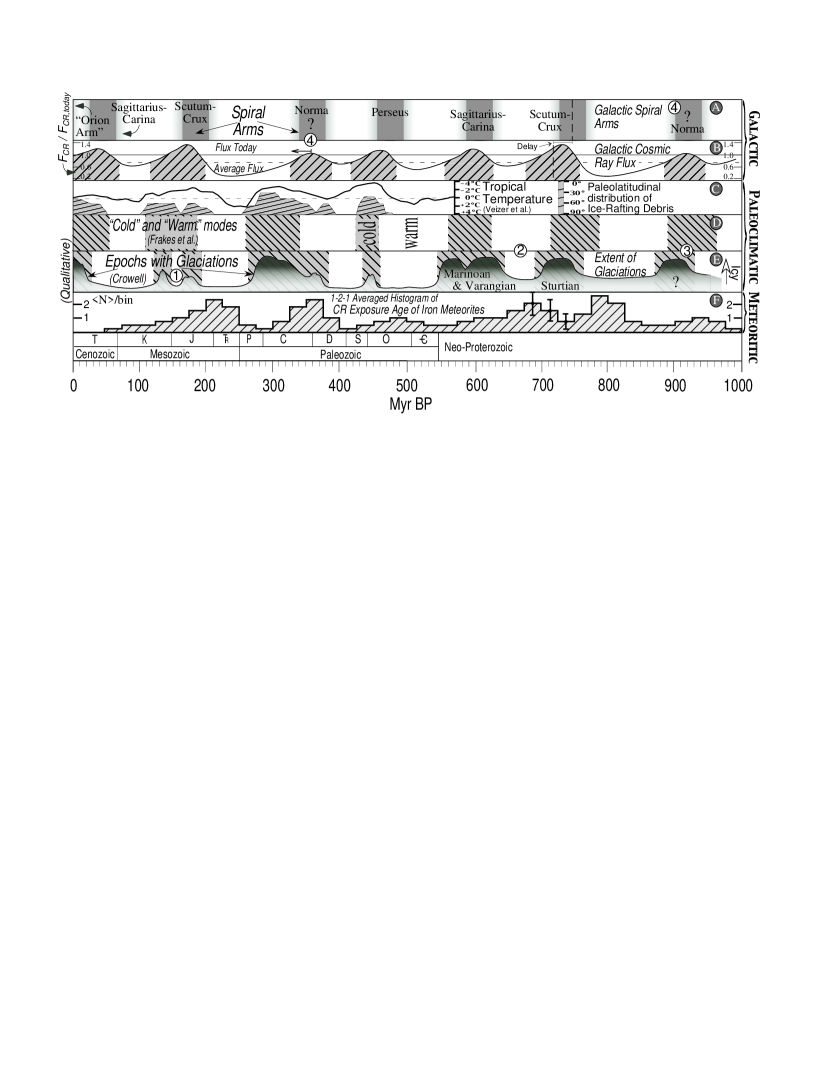
Figure 10: Earth’s recent history. The top panel (A) describes past crossings of the Galactic spiral arms assuming a relative pattern speed of $\Omega_{p}-\Omega_{\odot}=-11.0$ km sec^-1 kpc^-1(which best fits the IAEs). Note that the Norma arm’s location is actually a logarithmic spiral extrapolation from its observations at somewhat smaller Galactic radii Leitch & Vasisht, (1998); Taylor & Cordes, (1993). The second panel (B) describes the Galactic CRF reaching the solar system using the CR diffusion model, in units of the current day CRF. An important feature is that the flux distribution around each spiral arm is lagging behind spiral arm crossings. This can be seen with the hatched regions in the second panel, which qualitatively show when IAEs are predicted to occur if the critical CRF needed to trigger them is the average CRF. Two dashed lines mark the middle of the spiral crossing and to the expected mid-glaciation point. Panels (C) (D) and (E) describe the paleoclimatological record of the past Eon. The solid line in panel (C) depicts the tropical sea surface temperatures relative to today, as inferred from calcite and aragonite shells in the past $\sim 550$ Myr Veizer et al., (2000). The filled areas describe the paleolatitudinal distribution of ice rafted debris Veizer et al., (2000). Panel (D) and (E) qualitatively describes the epochs during which Earth experienced ice-ages, the top part as described by Frakes et al., (1992), while the bottom one by Crowell, (1999). The Phanerozoic part of panel E is directly taken from Crowell, (1999). The Proterozoic part is its extension using the data in Crowell. It has an elevated base level (since glaciations were more common) and it describes the main epochs of extended glaciations. By fine-tuning the actual pattern speed of the arms (relative to our motion) to best fit the IAEs, a compelling correlation arises between the two. The correlation does not have to be absolute since additional factors may affect the climate (e.g., continental structure, atmospheric composition, etc.). Panel (F) is a 1-2-1 smoothed histogram of the exposure ages of Fe/Ni meteors. The meteor exposure ages are predicted to cluster around epochs with a lower CRF flux.

IV.2 Comparison with CRF record in Fe/Ni meteorites

A smoking gun, which would unequivocally demonstrate that the spiral-arm $\rightarrow$ cosmic-ray $\rightarrow$ climate connection is real, would be a “historic” record which would reveal that the CRF was indeed variable. Such an independent record could on one hand show that the CRF varied as expected from the spiral arm CR diffusion model, while on the other hand, that it varied synchronously with the appearance of ice-age epochs on Earth. In §II.4, a new method was developed with which we could extract the actual CRF history.

It was found that the CRF record shows a clear variability signal with a periodicity of $143\pm 10$ Myr. This variability is consistent both in periodicity and phase, with the predictions of the CR diffusion model which incorporates the spiral arms, of which the expected periodicity is $134\pm 25$ Myr. This is clearly demonstrated in fig. 4.

Since the periodicity in the CRF is more accurately known than the spiral arm pattern speed (because of both statistical and systematic errors), it is a much stronger tool to use when comparing the astronomical data with the geological one. Indeed, the periodicity of the IAEs as can be obtained from table 2, is found to be $145.5\pm 7$ Myr, which nicely agrees with the aforementioned CRF period of $143\pm 10$ Myr. This agreement in phase can also be seen in fig. 4 where the clusters of exposure ages tend to be anti-correlated with the occurrence of IAEs.

The last result is of course trivial once we consider that the CRF as recorded in Fe/Ni meteorites was already shown to agree with the predicted CRF using the galactic model and that the latter was shown to agree both in phase and period with the occurrence of IAEs.

The implications are not only statistical, but also qualitative, since the above agreements provide a “missing link” which explicitly point to the cosmic rays as being the culprit in climatic variability. Namely, it looks as if we found the smoking gun we sought after.

IV.3 The past Star Formation rate history and ice-epochs

A summary of the past star formation rate history was given in §II.3. It is summarized again in figure 2, together with the epochs during which Earth witnessed ice-ages.

The main correlation apparent from the graph is the paucity in the MW’s star formation rate between 1 and 2 Gyr BP (with the cautionary note of §V.1), which coincides with a long interval on Earth during which there were no apparent glaciations whatsoever. On the other hand, during the last eon, and the one between 3 and 2 Gyrs BP, Earth did have glaciations and the SFR was higher. Although it is speculative, this variability in SFR appears to correlate with perigalacticon passages of the LMC, and in fact, also with the SFR in the LMC.

For the SFR on shorter time scales, we have to rely on the cluster data (see fig. 2), or the mass distribution of nearby stars Scalo, (1987), which have a ‘finer’ resolution than the SFR calculated using chromospheric ages of nearby stars. These show that at 0.3 Gyr BP, there was a higher than average SFR. A second peak appearing in the cluster data, could have occurred at 600 Myrs BP (though the data is not statistically significant). Interestingly enough, the IAE 300 Myrs and 600-700 Myr BP appear to be correlated with more extensive glaciations: The recent peak correlates with the Carbonaceous-Permian IAE, while the peak at 600-700 Myrs coincides with the late Neo-Proterozoic IAE, both of which were relatively extensive.

Although it is hard to quantify the statistical significance of the SFR-climate correlation, the fact that the results are consistent with that expected from the theory is reassuring (though see the possible caveats in §V.1). Namely, we expect and indeed find the relation: Higher star formation rate $\rightarrow$ more CR generation $\rightarrow$ colder climate.

V Discussion

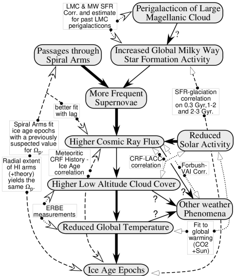
Figure 11: The model for how the Galaxy affects the ice ages. Solid arrows reflect physical cause and effect. Bold lines are hard to dispute relations while thin lines are reasonable relations based on observational correlations. Arrows with question mark are unknown though possible relations. Dotted and dashed arrows reflect observational correlations which relate two (or more) physical ingredients. Dotted lines are previously found correlations while dashed lined are correlations obtained and described here.

The basic evidence presented supports a picture in which climate on Earth is affected by our changing location in the Milky Way, by way of a variable cosmic-ray flux. The various physical links and the observational evidence which support these relations are charted in fig. 11. One should note the redundancy in the key results which support this conclusion. These are the temporal correlations between the expected spiral arm crossing, the variable CRF observed in Iron meteorites, and the appearance of ice-ages on Earth.

For nominal values taken, we find an effect of +5 to -10^∘K relative to today, however, there are some large uncertainties. A factor of order unity arises from the uncertainty in the cloud – temperature relation. Another factor of order unity arises from the uncertainty in the relation between the Cosmic Ray flux itself and the cloud cover. The normalization of the latter can be achieved using the solar modulation with the complication however that it modulates CR fluxes of different energies differently. Nevertheless, it is clear that the low altitude nature of the CRF-climate effect, requires the relevant energies to be high ($\gtrsim 10$ GeV). Thus, a normalization factor of 2 higher or lower between the CRF and cloud cover connection is conceivable. A consistency check which verifies that the net CR $\rightarrow$ LACC $\rightarrow$ temperature relations that we obtained are reasonable, is using global warming in the past century to directly calculate the CR $\rightarrow$ temperature relation.

The last source for an inaccuracy in the CR $\rightarrow$ temperature relation arises because we extrapolate a several percent effect to several tens of percent. Without knowing the physical process behind the effects of the CRs on the atmosphere. We cannot know, for example, whether the effect does not saturate at small relative changes.

Although the actual links presented here relate the CRF to the changing global temperature, there is good reason to believe that the link itself is through a variable cloud cover. First, such a link was already empirically observed in the form of a direct correlation between the low altitude cloud cover and the CRF. Moreover, the observed correlation yields a radiation driving that is more than sufficient to explain the occurrence of ice-ages, but also the changes in the past century which are attributable to solar activity. In other words, other pathways relating the CRF with temperature are not required at this point, but clearly, we cannot rule them out.

If the link is not through the variable low altitude cloud cover (or if an additional link exists), then lower energy CRs could be affecting the climate as well. In this case, the effects that a dense ISM cloud has on the heliosphere Begelman & Rees, (1976) could clearly be affecting the climate as well since these events will drastically change the low energy charge particle flux reaching Earth. In such a case, the ice-age epochs could be dotted with relatively short events during which the climate changes dramatically for the typical durations it takes to cross such ISM clouds (either heating or cooling, depending on whether the reduced flux of solar CRs or the increased galactic CRs are more important, and on the actual climatic mechanism).

For example, if relatively low molecular cloud densitites of 100 cm³ can significanty alter the heliospheric structure and with it the low energy cosmic ray flux reaching Earth, and if the latter do affect climate, then an effect could actually take place for $10^{7}$ years, which is the typical duration it would take the solar system to cross a 100 pc cloud. In any case, These events are more likely to be synchronized with the spiral arm crossing itself and not lagged behind it.

One should also note that passing through young stellar nurseries could also locally increase the intrinsic CRF reaching the solar system. Through the low altitude cloud cover connection, this would cause dramatic short term reduction in the temperature. Namely, the long ice-age epochs could be dotted with short events of even colder climate.

The CR diffusion model developed here, has shown that the spiral structure should be incorporated in CR diffusion models since qualitative and quantitative corrections are otherwise missed. (The model described here is nowhere as complex as some CR models, so neither it nor previous models should be the final word). Moreover, even the spiral structure itself deserves a more detailed description. For example, the spiral arms were assumed to be straight “rods”. A much bigger effect could however arise from the approximation that the diffusion coefficient is the same everywhere. However it is expected that the diffusion coefficient will be lower in the denser spiral arms. This could have an effect on the entrapment of the CR in the spirals for a longer time, thereby increasing the CR density contrast.

To the extent that spiral density wave theory applies to the Milky Way’s spiral arms, the spiral structure of the outer parts of our galaxy ($R\gtrsim R_{\odot}$) is apparently pinned down. Therefore, it should serve as an outer boundary when Milky Way models are constructed. We found that the structure between us and the center will however be different in nature. The reason is that the outer 4-arm spiral cannot extend much further inside the solar galactocentric orbit, though spiral arms are seen further inside the disk. This implies that models previously used to describe the galaxy with only one pattern speed are not sufficient. It could explain why previous results for the number were in contradiction.

Another interesting observation is that geology is now is a unique position to serve as a tool in the study of galactic dynamics. For example, it now appears that the life time of spiral arms is at least $\sim 900$ Myr or 1.5 rotations. This is expected whether the spiral arms are a ‘transient’ phenomenon or a more permanent one (an issue which is still not settled). Should however the same periodicity be found in the glaciations 2-3 Gyr BP, then a very interesting constraint could be placed on the spiral dynamics.

Moreover, using temporal variability (either in the CRF or the glaciations), we have managed to measure the spiral pattern speed more accurately than using pure ‘astronomical’ methods. The accuracy with these temporal methods is in fact large enough that one needs to consider that the corrections from our diffusion in the galaxy results in an offsetted pattern speed, since this correction is of order the error bars themselves or even larger. This is the first time a temporal record (instead of a “snapshot”) is used to study galactic dynamics.

It is also worth noting that the effects of terrestrial magnetic reversals on climate are probably not dramatic as could be naively expected, even though the total CRF is significantly increased in such events. The main reason is that the LACC-CRF connection is observed in low altitudes and low latitude clouds. This necessarily implies that high energy CRs are those mostly responsible for the effect. These CRs reach the equator irrespective of the strength of Earth’s magnetic field. For example, if we look at the original results of Compton, (1933), we find that the change in atmospheric ionization at sea level varies by only $\sim 14\%$ between the magnetic equator and poles. Therefore, even if the Earth’s magnetic field were to completely vanish, our estimates for the temperature change would correspond to at most a 1 to 2^∘K reduction in temperature. This is corroborated by the Laschamp event (36-41.5 kyr BP) during which the terrestrial field was significantly reduced Guyodo & Valet, (1996). During the event, an increased ¹⁰Be and ³⁶Cl flux was recorded in Greenland ice cores, but no statistically significant climatic effect was recorded in ¹⁸O or CH₄ Wagner et al., (1999). This is expected considering that the temperature variability recorded in the ice cores, either before or after the event, is much larger than 1 to 2^∘K.

V.1 Caveats

The picture presented here includes many elements which add up to what appears to be a coherent picture. Unfortunately, most if not all observational data used here, whether astronomical, meteoritic, or paleoclimatological does not come without a grain of salt. The purpose of this section is to discuss and summarize the limitations of the data and possible caveats. Hopefully, by illuminating where the problems may rest, future research will try to address these points with the goal of resolving them.

Paleoclimatological Data: By far, the least conclusive data used is the past evidence for the occurrence of glacial epochs. In particular, it is debated whether ice-age epochs in the past billion years have been periodic or not. Some claim that a periodicity exists Williams, (1975); Frakes et al., (1992), while others claim that insufficient data exists to claim periodicity Crowell, (1999). Besides the timing of the glaciations (which becomes poorer as we go back in time), there is also the problem that ice-age epoch severity clearly varies from one IAE to the next. For example, the mid-Mesozoic ice-age epoch ($\sim 150-170$ Myr BP) was clearly very ’mild’ compared to other IAEs. On the other hand, from 800 Myr BP until well after 600 Myr BP, it seems that Earth continuously had some sort of glaciations present, with colder episodes around 600 and 750 Myrs BP. In fact, around 750 Myrs BP, there is evidence for glaciations at sea level and equatorial latitudes. That is, glaciations more extensive than anything seen by Earth at any period Hoffman et al., (1995). In addition to the problem of a varying severity or extensiveness, there is also the question of length. For example, the Carboniferous-Permian glaciations were 3 or 4 times the duration of the short Silurian-Devonian glaciations that preceded. These problems are also noted in figure 10. Note however, that even though the above problems exist, the timing of the IAEs of Frakes and of Crowell are generally consistent with each other.

Another point which one might note at first glance of fig. 10 is that although the general agreement is good, there are some inconsistencies between spiral crossings and actual occurrence of IAEs. As previously explained, this should not be a concern because of several reasons. First, the actual spiral crossing signal is expected to have a ‘jitter’ because of the epicyclic motion of the solar system. Second, since the Milky Way is not a ‘grand design’ spiral galaxy, the spiral arms are not the perfect geometrical objects they are assumed to be. In particular, ‘gaps’ in which the spiral arms are weaker or arm ‘spurs’ which fill the inter-spiral-arm with young CR producing stars are not uncommon. The lifetime of the spurs, however, is less than a galactic orbit. Therefore, they are not expected to repeat themselves after 4 spiral crossings. Third, geological factors are also expected to be important in climate change. For example, the changing continental structure might free the poles of land masses, and could even allow temperate ocean currents to reach the poles. This can hinder Earth from triggering the formation of ice sheets.

The above factors appear to be particularly important in the last IAE. Although the main spiral arm crossing took place about 50 Myr BP, the last IAE started only ‘recently’, about 30 Myrs BP. The reason we are now in an IAE is easy to explain since we are in the Orion armlet. This leaves the question of why didn’t the IAE begin as the solar system entered the Sagittarius-Carina arm? This could be a result of factors intrinsic to Earth. The main factors often cited as the reason that the latter part of the Cretaceous was one of the warmest periods in Earth’s history (e.g., Huber, (1998)), are that the land mass did not occupy the poles and that the global sea level was highest than ever (thus moderating the temperatures). Nevertheless, if careful attention is given to the temperature variations over the Cretaceous and Cenozoic (e.g., Huber, (1998), Zachos et al., (2001)) then it is apparent that the temperature variations were more complicated than a simple monotonic cooling. At 90 Myr BP, the average global temperature peaked. But in the 10 Myr preceding the K/T transition (at 66 Myr BP), the temperature dropped by more than 5^∘K. The temperature rose again by several degrees, and peaked at around 52 Myr BP, after which it declined (though non-monotonically) until present, when extensive glaciations are common. It is tempting to attribute the first minimum to the crossing of the Sagittarius-Carina arm. Namely, Earth did experience a reduced global temperature however, because of intrinsic effects (and perhaps because the arm at the point of crossing was not prominent), the temperature did not fall enough to trigger glaciations. After the Sag.-Car. arm was crossed, the temperature rose again. However, the Orion arm and the changing global conditions caused a large cooling afterwards.

Although the above explanation is far for satisfactory, it shows that the model developed in the paper is incomplete. In particular, it is probably the case that “standard” paleoclimatic factors intrinsic to Earth are as important at determining the global climate as the external effect of the cosmic rays.

Astronomical Data: We have used in the analysis astronomical data describing the spiral structure, spiral pattern speed and star formation rate. Unfortunately, there is still no consensus on any one of them.

Although the analysis presented here, and in particular the meteoritic exposure age data, seems to be consistent with the various spiral arm indicators located outside the solar galactocentric radius, if we look inwards, the structure and dynamics appear significantly less clear. In particular, there are convincing arguments which indicate that the solar galactic orbit is close to co-rotation (e.g., Mishurov & Zenina, (1999)). If true, it would imply a spiral arm pattern speed similar to $\Omega_{\odot}$, instead of a much larger $\Omega_{\odot}-\Omega_{p}$, as found here. Obviously there is a contradiction that should be resolved. One possibility raised in §2, is that the Milky Way has more than one set of spiral arms with different pattern speeds. This is required if the outer parts have a low pattern speed, and it would explain the large confusion that exists in the field. Clearly, this issue is still not resolved and deserves more attention than it has received in recent years.

Interestingly, having two sets of spiral arms also has the potential of explaining the ‘staggered’ severity and length seen in the ice-age epochs. Namely, it could be that we are also affected by the spiral structure internal to our galactocentric radius, and that its period relative to us is about 300 Myr. Nevertheless, this is quite speculative, and it is not unlikely that this staggered behavior arises from terrestrial factors. For example, atmospheric CO₂ levels around the Carboniferous-Permian period were several times smaller than the other periods in global history with the exception of recent geological times.

Another caveat has to do the location of the Norma arm at our galactic radius. This location was obtained through a logarithmic extrapolation from where it is observed at smaller galactic radii (à la Leitch & Vasisht, (1998); Taylor & Cordes, (1993)). However, as discussed in §II.2.3, there are good reasons to believe that the structure within the solar circle is different from the one at our radius and outwards. This would imply that the Norma arm seen at smaller radii is not necessarily part of the same structure that should be localized between the Scutum-Crux and the Perseus external arms, on the other side of the galaxy. If so, the preferred crossing of this arm would be later by $\sim 40$ Myr, as its preferred location would be symmetrically in between the adjacent arms. If we look at fig. 10, we see the this will in fact increase the agreement between the predicted location of the spiral crossings around 300 and 900 Myr BP and both the time of occurrence of the relevant IAEs and the observed CRF variability. It would not explain though the extent the the Carboniferous-Permian IAE.

A third astronomical caveat has to do with the star formation rate. The SFR with which the glacial activity on Earth was compared with was that of Rocha-Pinto et al., (2000b), which is also consistent with various other authors. However, like most results quoted here, there are a few contradictions published in the literature, which, if verified will pose a problem for the model presented here. In particular, Hernandez et al., (2000) have used the Hipparcos astrometric data combined with detailed theoretical isochrones to obtain the SFR of nearby stars (which due to diffusion corresponds to the azimuthally averaged SFR on periods over a billion years). The gross features they obtained are inconsistent with other analyses (for example, with Rocha-Pinto et al., (2000b)). In particular, the SFR they obtained decreased from 2 Gyr BP until today with only relatively small ‘wiggles’. Moreover, they did not find a dip between 1 and 2 Gyr BP. Thus, an independent study of the Hipparcos data should be pursued in order to resolve this discrepancy.

Meteoritic Data:

Regarding the variable CRF from exposure age data, one should note the following. Just the data showing the clustering of meteorites by itself can be interpreted in several ways. The clustering can either be a manifestation of a variable CRF, or, it can be a genuine clustering of exposure ages.

Since the stable isotopes used in the currently employed methods for exposure dating Fe/Ni meteorites (e.g., ³⁶Ar, ²¹Ne, ⁴¹K), are all formed primarily from Galactic CRs Michel et al., (1995), the observed data could not be a result of a variable solar CRF. Thus, within the interpretation of a variable CRF, the observed variability can arise from either an intrinsic variability in the Galactic CRF (as assumed in this work) or a variability induced by a variable heliosphere. In the second possibility, one can accredit the exposure data to a variable solar wind (with the observed periodicity of $\sim 150$ Myr) and attribute the observed correlated climatic variability to the solar variations. Although possible, this option which has far reaching implications, seems less reasonable because of the correlation of the CRF and climatic data with the observed galactic pattern speed with the same period. Namely, it would be strangely coincidental if the sun were to have a variability that is synchronized with the spiral arm crossings.

The third possibility for interpreting the exposure age data is that the CRF was constant and that the clustering in the exposure ages is real. Namely, episodes in the past in which asteroids or comets were more likely to break apart existed periodically. This is not an unreasonable hypothesis. For example, one could claim that the Oort cloud is perturbed more often during spiral arm crossing, injecting more comets to the inner solar system, thus breaking apart more asteroids. Moreover the more numerous debris could reasonably have climatic effects as well (see §I). Within the context of this interpretation, clusters of meteoritic exposure ages, as well as the ice age epochs, should coincide with the spiral arm crossing with no phase lag. The data however shows that the clusters are not in phase with either the spiral crossings or the IAEs, nor are the IAEs in phase with the spiral arm crossings.

Thus, the most consistent picture arises if we interpret the exposure age clusters as a result of an intrinsically variable Galactic CRF. One way to prove this, is to look at age distributions of Iron meteorites which were CR exposure dated using a method in which the stable isotope that accumulates is sensitive primarily to the solar cosmic-ray flux. The reason is that if the clustering is real (and not due to a variable Galactic CRF) then the same clustering will appear in solar sensitive dating methods. This would also be useful to rule out the possibility that the apparent variations are not Galactic in origin, but are induced by solar variability instead. If this unlikely case is true (which would imply that IAEs are linked with solar variability, since the CRF-climate correlation exists irrespectively), then the opposite clustering will be present in solar sensitive data. With the most reasonable interpretation, though, no clustering is predicted in the solar sensitive data, once it could be obtained.

VI Summary and Conclusions

The thesis presented here relates the following topics: The Milky Way dynamics, Cosmic Ray diffusion in the Galaxy, the CR record in Iron meteorites, the effect of Cosmic Rays on climatology, and glaciology. This is achieved by considering the intimation that CRs can affect the global cloud cover and that the CR flux from the Galaxy should be variable. Before summarizing the main conclusions relating the above topics, “preliminary” conclusions on each of the various topics can be drawn from the background analysis.

Milky Way Dynamics: By studying the 4-arm structure seen in HI, extending to roughly $2R_{\odot}$, stringent constraints can be placed on the spiral pattern and dynamics of the Milky Way:

1. Since observations of HI outside the solar circle suffer no velocity-distance ambiguity, the observations of 4-spiral arms should be considered robust. If one further assumes that these arms are density waves (which is by far the most consistent explanation for spiral arms) then these arms cannot extend further out than the 4 to 1 Lindblad resonance. This implies $\Omega_{p}\lesssim 16\pm 2.5$ km sec^-1 kpc^-1. This number agrees with roughly half the determinations of $\Omega_{p}$, which cluster around this value.

2. Several additional considerations point to the above value being not an upper limit for $\Omega_{p}$, but the actual value of it.

3. The 4-arm spiral cannot extend much further in from the solar galactocentric radius. Several possibilities were raised. Since the MW has a bar, at least two different pattern speeds exist in the MW.

4. On a more speculative note, long term activity in the star formation rate appear to correlates with activity in the LMC and possibly with its perigalacticon passages, suggesting that long term star formation in the Milky Way and LMC are related.

CR Diffusion:

1. Since CR sources are clearly more common to the Galactic spiral arms, models for CR propagation in the MW should take this fact into account. Otherwise, significant discrepancies can arise. In particular, quantities such as the “age” of the cosmic rays reaching Earth can be distorted.

2. For typical diffusion model parameters, the CRF is expected to vary by ${\mathcal{O}}(1)$, which is consistent with radio observations of external spiral galaxies.

3. The distribution of CRs is both lagging behind the spiral crossings (when defined for example by the HII regions) and skewed towards later times. The skewness arises from the asymmetry introduced by the spiral arm motion. The lag in the peaks arises because the SN explosions are lagging the ionizing photons that produce the HII regions, and which were used here (and in Taylor & Cordes, (1993)) to define the location of the arms.

CR record in Iron meteorites:

1. The “standard” method for extracting historic variability of the CRF, by comparing ${}^{41}{\rm K}/^{40}$K dating to dating with a short lived unstable nucleotide (such as ${}^{10}\mathrm{Be}/^{21}\mathrm{Ne}$) are effective only at extracting “recent” changes (over several Myrs) or secular changes over longer durations, but they are not effective at extracting the signal expected from the periodic variability of the spiral arm passages.

2. An effective method for finding the periodic CRF variations is a statistical analysis of CR exposure ages. It assumes that the rate at which “new exposed surfaces” appear in Iron meteorites does not vary rapidly.

3. This method shows that the exposure age data is consistent with it being periodic, with a period of $143\pm 10$ Myr, and a CRF contrast of $\max(\Phi)/\min(\Phi)\gtrsim 3$. It uses 50 meteorites which were dated only with ${}^{41}{\rm K}/^{40}{\rm K}$. The method reveals that statistically, it is unlikely that the meteor exposure ages were generated by a random process.

The Milky Way – Climate connection: By comparing the above findings to the appearance of glaciations on Earth, the following conclusions can be deduced:

1. Periodic glaciation epochs on earth in the past 1 Gyr can be consistently explained using the proposed scenario: Periodic passages through the Galactic spiral arms are responsible for an increased CRF, an increased LACC, a reduced global temperature and consequent ice-ages.

2. Long term glaciation activity is apparently related to the global SFR activity in the Milky Way. This may be related to LMC perigalacticon passages which would imply that the nearby extragalactic environment could be added to the factors affecting the global climate.

The evidence upon which the above conclusions were based, is the following:

1. The period with which spiral arm passages have occurred using the HI data alone (and which should also correspond to the CRF period), is $163\pm 50$ Myr. By combining the result of the 8 total measurements that scatter around this value, the predicted spiral arm crossing period is $134\pm 22$ Myr. The period with which the CRF appears to vary using Fe/Ni meteorites, is $143\pm 10$ Myr. The period with which glaciations have been observed to reoccur on Earth is $145.5\pm 7$ Myr on average. Clearly, all three signals are consistent with each other.

2. By comparing the actual prediction for the location of the spiral arms to the glaciations, a best fit of $143\pm 5$ Myr is obtained. The phase of all the three signals using this periodicity is then found to fit the predictions. In particular:

   • The average mid-point of the glaciations is lagging by $33\pm 20$ Myr after the spiral arm crossing, as is predicted ($31\pm 8$ Myr, from a possible range of $\pm 75$ Myr).

   • The CR exposure ages of Iron meteorites cluster around troughs in the glaciations.

3. A random phenomenon for the appearance of glaciations is excluded with very high statistical significance.

4. Long term variability in the appearance glaciations correlates with the observed SFR variability of the Milky Way. In particular, the lack of apparent glaciation between 1 and 2 Gyr BP, correlates with a particularly low SFR in the milky way (less than half of today), while a high SFR rate between 2 and 3 Gyr BP (with a peak towards 2 Gyrs), correlate with the glaciations that Earth experienced between 2 and 3 Gyrs BP.

Additional conclusions: More conclusions can be reached by considering the above results. They do not pertain to climatic variability, but instead, they can be drawn by assuming that long term climate variability is indeed a measure of CRF variability, as the above results seem to endorse.

1. Once more accurate “Eulerian” measurements of the Galactic pattern speed will be available, interesting constraints could be placed on solar migration in the galaxy. This is achieved by comparing the “Eulerian” measurements of the pattern speed to the “Lagrangian” pattern speed (as measured by the moving solar system), which is now known to an accuracy of $\pm 3\%$.

2. The variability observed in the CRF record in Iron meteorites (see point 10) can be used to place constraints on models for the CR diffusion in the Milky Way. This is in addition to the currently used constraint on the survival ratio of spallation products (primarily Be). Thus, from CRF variability, we find $D\lesssim 2\times 10^{28}{\rm~{}cm}^{2}/{\rm sec}$ and $l_{H}\lesssim 2$ kpc.

3. The 4-arm spiral pattern has been stable for at least a billion years. A better understanding of past Glaciations (e.g., 2-3 Gyrs ago) could place interesting constraints on the lifetime of the spiral arms which cannot be done by any other means.

As apparent from the above list, there are several interesting ramifications to the picture presented here. However, one which bears particular interest on global warming and which was not discussed here, is that it now appears even more plausible that cosmic rays indeed affect the global climate, as suggested for example by Ney, (1959), Tinsley & Deen, (1991), and Svensmark & Friis-Christensen, (1997). This implies that it is now more plausible that solar variations are affecting climate through modulation of the cosmic ray flux. This would explain an important part of the global warming observed over the past century. It is because of this important aspect, in particular, that we are obligated to iron out the still unclear points raised in the caveats section, whether it be the paleoclimatological record, the possible mechanism by which cosmic rays affect climate, or our astronomical understanding of the structure and dynamics of the Milky Way.

Appendix A: The “Age” of cosmic rays in the spiral arm diffusion model

The tightest constraint on different types of CR diffusion models in the galaxy can be placed by comparing their predictions to the expected ratio between ¹⁰Be, which is a radioactive isotope, to ⁹Be, which is stable. Both nucleotides are formed by CR spallation of mainly C, N and O.

In a leaky box model, the ratio at steady state between the density of specie $i$ of a stable isotope to that of an unstable isotope $j$, can be obtained from eq. 5. It is:

$${N_{j}\over N_{i}}={{\tilde{Q}}_{j}\over{\tilde{Q}}_{i}}{\tau_{r}\over\tau_{e,lb}+\tau_{r}}$$ (18)

where $\tau_{r}$ is the decay rate of the unstable isotope and $\tau_{e,lb}$ is the leaky box decay rate. It is assumed that the spallation time is much longer than $\tau_{e,lb}$ or $\tau_{r}$.

Different measurements for the isotope ratio ¹⁰Be/Be are $6.4\pm 1.5$% Wiedenbeck & Greiner, (1980), $3.9\pm 1.4$% Simpson & Garcia-Munoz, (1988), $4.3\pm 1.5$% Lukasiak et al., (1994). These ratios respectively yield a $\tau_{e,lb}$ of $18.1^{+8.1}_{-5.0}$ Myr, $30.3^{+21.5}_{-10.0}$ Myr, and $27.1^{+18.9}_{-9.0}$ Myr Lukasiak et al., (1994). We shall adopt an age of $24^{+12}_{-6}$ Myr which is the measurements’ average and a somewhat conservative error which is the maximum error divided by $\sqrt{3}$.

In the spiral arm diffusion model, there is no steady state, so the calculation of the ratio ${N_{j}/N_{i}}$ is more complicated.

To simplify the calculation, we utilize the previously obtained result that to a reasonable approximation, the effects of the boundaries is to have the CR distribution decay exponentially, not unlike the leaky box model. (Namely, we approximate the $\vartheta_{4}$-function as an exponent). This implies that the number density of the CRs that were emitted at a given time decays exponentially with a time constant of $\tau_{e}=l_{H}^{2}/(2.47D)$. Thus, the density of specie $k$ which is the parent nucleotide of the spallation products (namely, C, N and O producing the Be) and which where generated at time $t^{\prime}$ will decay as $\exp(-(t-t^{\prime})/\tau_{e})$.

The two (united) equations that describe the production and decay of the spallation products formed by parent nucleotides that were generated at time $t^{\prime}$, are therefore:

$${dn_{i,j}\over dt}=-{n_{i,j}\over\tau_{e}}+q_{i,j}\exp\left(-{t-t^{\prime}\over\tau_{e}}\right)-\left\{0~{}{\rm or}~{}{n_{j}\over\tau_{r}}\right\}.$$ (19)

$n_{i,j}(t,t^{\prime})$ is the density of specie $i$ (stable) or $j$ (unstable) that were generated from nucleotides of type $k$ at $t=t^{\prime}$.

The solution to the two equations with the assumption that $n_{i,j}(t=t^{\prime})=0$ (namely, that the spallation products are not found initially in the accelerated CRs) are:

$$n_{i}(t,t^{\prime})=q_{i}\exp(-\Delta t/\tau_{e})\Delta t$$ (20)

$$n_{j}(t,t^{\prime})=q_{j}\left[\exp\left(-{\Delta t\over\tau_{e}}\right)-\exp\left(-{\Delta t\over\tau_{\mathrm{eff}}}\right)\right]{\tau_{e}\tau_{\mathrm{eff}}\over\tau_{e}-\tau_{\mathrm{eff}}}$$ (21)

with $\tau_{\mathrm{eff}}^{-1}\equiv\tau_{r}^{-1}+\tau_{e}^{-1}$, and $\Delta t\equiv t-t^{\prime}$. If we write eq. III.2 as:

$$\Phi(x,z=0,t)=\int_{-\infty}^{t}dt^{\prime}G(x,t,t^{\prime})\vartheta_{4}\left(0,\exp\left[-\tau/(\Delta t+\delta t)\right]\right)$$ (22)

with $\delta t\equiv\sigma_{z}^{2}/(2D)$, then:

$$N_{i}\approx q_{i}\int_{-\infty}^{t}dt^{\prime}G(x,t,t^{\prime})\exp\left[-(t-t^{\prime}+\delta t)/\tau_{e}\right]$$ (23)

and

$$N_{j} \approx q_{j}\int_{-\infty}^{t}dt^{\prime}G(x,t,t^{\prime}){\tau_{e}\tau_{\mathrm{eff}}\over\tau_{e}-\tau_{\mathrm{eff}}}$$ (24)

$$\times\left[\exp\left(-{\Delta t+\delta t\over\tau_{e}}\right)-\exp\left(-{\Delta t+\delta t\over\tau_{\mathrm{eff}}}\right)\right].$$

If we define ${\mathcal{R}}\equiv{N_{j}/N_{i}}$, and compare the above result to those of the leaky box model, then the effective leaky box decay time $\tau_{e,lb}$ is related to $\tau_{e}$ and ${\mathcal{R}}$ through:

$$\tau_{e,\mathrm{lb,eff}}=\tau_{e}\left({1\over{\mathcal{R}}}-1\right).$$ (25)

This allows us to calculate the effective age of the CRs that the Be isotope ratio would correspond to in a “leaky box” model.

Appendix B: Systematic errors from diffusion and epicycles in the solar orbit

In this work, we compare two completely different types of measurements of the spiral pattern speed. On one hand, there are the present day astronomical measurements of the spiral pattern speed. On the other hand, there are the temporal records of passages through spiral arms—either as recorded in the ice age reoccurrence, or as recorded in the variable CRF in Iron meteorites. The two types of measurements should yield the same result if the solar orbit is stable at its current radius. This is not the general case however, we are therefore required to estimate the error that can arise when comparing the two.

Although collisions that drastically change the solar orbit are statistically unexpected, the Solar system undergoes many small angle deflection such that its orbit parameters slowly diffuse. Namely, the “Lagrangian” record of spiral arm crossings, as measured by the moving solar system, need not be exactly the same as a test “Eulerian” particle would experience when fixed at the current $R_{\odot}$.

The solar motion itself can be broken down to a circular motion of the guiding center at radius $R_{m}$ and an epicyclic motion at frequency $\kappa$ and radius $a_{R}$.

According to Wielen, (1977) and Wielen et al., (1996), both amplitudes undergo diffusion, according to:

$$\Delta R_{\mathrm{m,rms}}\equiv\sqrt{\left<\Delta R_{m}^{2}\right>}=\sqrt{D_{m}t}~{}~{};~{}~{}D_{m}=\mathrm{(0.72~{}{kpc})^{2}/Gyr,}$$ (26)

and

$$\Delta a_{\mathrm{R,rms}}\equiv\sqrt{\left<\Delta a_{R}^{2}\right>}=\sqrt{D_{a}t}~{}~{};~{}~{}D_{a}=\mathrm{(0.84~{}kpc)^{2}/Gyr},$$ (27)

for $t>10^{8}$ yrs. Also relevant, is the “diffusion” along the azimuthal angle direction. This is given by:

$$\Delta S_{\mathrm{rms}}\equiv\sqrt{\left<\Delta S^{2}\right>}=\sqrt{D_{s}t^{3}}~{}~{};~{}~{}D_{s}=\mathrm{(12.7~{}kpc)^{2}/Gyr^{3}}.$$ (28)

If we look at a given time $t$ before present, the uncertainties in $R_{m}$ and $S$ will be given by the above formulae. The uncertainty in $a_{R}$ is a trifle more complicated. This is because we have the prior knowledge that at $t_{0}=4.5$ Gyr BP, $a_{R,0}=0$ while today it is $a_{R,1}=0.6~{}\mathrm{kpc}$. To calculate $\Delta a_{\mathrm{R,rms}}$, we calculate the probability of the solar system having a given $a_{R}$ at time $t$ before present. It is given by:

$$P(a_{R},t) =$$

$$\hskip-22.76219pt{\rm G(a_{R},\sqrt{D_{a}(t_{0}-t)})\rm G(a_{R}-a_{R,1},\sqrt{D_{a}t})\over\int_{-\infty}^{\infty}\rm G(a_{R},\sqrt{D_{a}(t_{0}-t)})\rm G(a_{R}-a_{R,1},\sqrt{D_{a}t})da_{R}}$$

with

$$\rm G(x,\sigma)\equiv{1\over\sqrt{2\pi}\sigma}\exp\left(-x^{2}\over 2\sigma\right).$$ (30)

Using this, we find that:

$$\Delta a_{R,\mathrm{rms}} = \sqrt{\int_{-\infty}^{\infty}a_{R}^{2}P(a_{R},t)da_{R}}$$

$$= \sqrt{(t_{0}-t)(D_{a}t_{0}t+(t_{0}-t)a_{R,1}^{2})\over t_{0}^{2}}.$$

This result is the expected amplitude of the epicyclic motion as a function of time before present.

The diffusion processes will translate into two types of errors. One is the measurement error in the location of each spiral arm. The second is an error arising when calculating the average pattern speed over several periods.

The main contribution to the error in each spiral arm location is due to the epicyclic motion of the solar system around the ‘guiding center’, at a typical period of 200 Myrs. This implies that each spiral arm crossing is inaccurately predicted. This translates into a phase shift within the spiral passages. The r.m.s. of the variation is:

$$\Delta\phi_{\mathrm{{a,rms}}}={\Delta a_{\mathrm{{R,rms}}}/\sqrt{2}\over\pi R_{\odot}\sin i},$$ (32)

assuming 4 arms inclined at an angle $i$, and that the r.m.s. of the “circular” epicyclic motions is $1/\sqrt{2}$ of the radius. For a 140 Myr period (which will be a typical value found), we obtain that the phase error ranges from $\Delta\phi_{\mathrm{rms}}=15\%$ today to $\Delta\phi_{\mathrm{rms}}=22\%$ at 800 Myr BP. For a typical spiral arm crossing period of 140 Myr, this translates into an error of 21 to 31 Myrs respectively.

If we measure the pattern speed by dividing the duration it takes for $N$ spiral passages, several errors appear. First, the solar orbit can diffuse in or out. This introduces two errors by itself. The first is a phase error. Averaged over $N$ spiral passages, it introduces a relative error of:

$$\Delta\phi_{\mathrm{m,rms,1}}={2\Delta R_{\mathrm{{m,rms}}}\over\pi NR_{\odot}\tan i},$$ (33)

where $\Delta R_{\mathrm{m,rms}}$ is the value expected after $N$ spiral passages. This will give an absolute error of:

$$\Delta\Omega_{\mathrm{m,rms,1}} = \Delta\phi_{\mathrm{m,rms,1}}\left|\Omega_{\odot}-\Omega_{p}\right|$$

$$= {2\Delta R_{\mathrm{m,rms}}\left|\Omega_{\odot}-\Omega_{p}\right|\over\pi NR_{\odot}\tan i}$$

$$\approx 0.4~{}\mathrm{km~{}sec^{-1}~{}kpc^{-1}}{\rm~{}~{}for~{}~{}}t=800~{}{\rm Myr}$$

in the relative pattern speed. The second error from the diffusion of the solar orbit arises from the fact that at a different orbit, the pattern speed it different. Again, averaged over $N$ spiral passages, it introduces an absolute error in the pattern velocity of:

$$\Delta\Omega_{\mathrm{m,rms,2}} = {\Delta R_{\mathrm{m,rms}}\Omega_{\odot}\over 2R}$$ (34)

$$\approx 1.1~{}\mathrm{km~{}sec^{-1}~{}kpc^{-1}}{\rm~{}~{}for~{}~{}}t=800{\rm~{}Myr}.$$

A phase error also arises from the diffusion along the orbit:

$$\Delta\Omega_{\mathrm{S,rms}} = \Delta\phi_{\mathrm{S,rms,1}}\left|\Omega_{\odot}-\Omega_{p}\right|={2\Delta S_{\mathrm{rms}}\left|\Omega_{\odot}-\Omega_{p}\right|\over\pi NR_{\odot}}$$ (35)

$$\approx 0.3~{}\mathrm{km~{}sec^{-1}~{}kpc^{-1}}{\rm~{}~{}for~{}~{}}t=800~{}{\rm Myr}.$$

The first two errors are maximally correlated (they would have been anti correlated if either $\Omega_{p}>\Omega_{\odot}$ or $i<0$, but not both), and they are almost uncorrelated with the last. Therefore, the total error is:

$$\Delta\Omega_{\mathrm{rms}} = \sqrt{\left(\Delta\Omega_{\mathrm{m,rms,1}}+\Delta\Omega_{\mathrm{m,rms,1}}\right)^{2}+\Delta\Omega_{\mathrm{S,rms}}^{2}}$$ (36)

$$\approx 1.5~{}\mathrm{km~{}sec^{-1}~{}kpc^{-1}}{\rm~{}~{}for~{}~{}}t=800~{}{\rm Myr}.$$

Some indication to the radial solar migration can be obtained from its anomalously higher metallicity than its neighbors. This is statistically not very significant, but it does bias our expectation for solar diffusion. By comparing the solar metallicity to the surroundings and taking into account the apparent radial gradient in metallicity in the Milky Way, Wielen et al., (1996) found that the sun has migrated outwards by $\Delta R_{0}=1.9\pm 0.9$ kpc. Namely, we expect that the probability for the formation radius $R_{0}$ of the sun be given by $\rm G(R_{\odot}-R_{0}-1.9~{}{\rm kpc},\sigma_{0}=0.9~{}{\mathrm{k}pc})$. Therefore, the probability at time $t$ before present, to find the solar system at a radius $R$ is given by:

$$P(R,t)={\int_{-\infty}^{\infty}K(R_{0},R,R_{\odot},t)dR_{0}\over\int_{-\infty}^{\infty}K(R_{0},R,R_{\odot},t)dR_{0}dR}$$ (37)

$$K(R_{0},R,R_{\odot},t) \equiv \rm G(R_{\odot}-R_{0}-\Delta R_{0},\sigma_{0})$$ (38)

$$\rm G(R-R_{0},\sqrt{D_{m}(t_{0}-t)})$$

$$\times\rm G(R_{\odot}-R,\sqrt{D_{m}t})$$

We then obtain that the expectation value for $R$ at time $t$. It is:

$$\left<R\right> = \int_{-\infty}^{\infty}RP(R,t)dR$$

$$= R_{\odot}-{D_{m}t\Delta R_{0}\over D_{m}t_{0}+\sigma_{0}^{2}}\approx|_{t=0.8~{}{\rm Gyr}}~{}R_{\odot}-0.25~{}\mathrm{kpc}$$

and its r.m.s. error at $t=800$ Myr is:

$$\Delta R_{\mathrm{rms}}^{2} \equiv \left<R^{2}\right>-\left<R\right>^{2}$$

$$= \int_{-\infty}^{\infty}R^{2}P(R,t)dR-\left(\int_{-\infty}^{\infty}RP(R,t)dR\right)^{2}$$

$$= D_{m}t\left(1+{D_{m}t\over D_{m}t_{0}+\sigma_{0}^{2}}\right)\approx|_{t=0.8~{}{\rm Gyr}}(0.59~{}{\rm kpc})^{2}.$$

Using the previous results, we obtain that for a measurement baseline spanning 800 Myrs BP until today, the difference between the “Lagrangian” and “Eulerian” measurements is

$$(\Omega_{\odot}-\Omega_{p})_{\rm Lag}-(\Omega_{\odot}-\Omega_{p})_{\rm Euler}\approx 0.54\pm 1.5~{}{\rm km~{}s^{-1}~{}kpc^{-1}}.$$ (41)

References

- Alvarez et al., (1980) Alvarez, L. W., Alvarez, W., Asaro, F., & Michel, H. V. 1980. Science, 208, 1095.
- Amaral & Lepine, (1997) Amaral, L. H., & Lepine, J. R. D. 1997. Mon. Not. Roy. Astr. Soc., 286, 885.
- Avedisova, (1989) Avedisova, V. S. 1989. Astrophys., 30, 83.
- Barry, (1988) Barry, D. C. 1988. Astrophys. J. , 334, 436.
- Bazilevskaya, (2000) Bazilevskaya, G. A. 2000. Sp. Sci. Rev., 94, 25.
- Beer et al., (2000) Beer, J., Mende, W., & Stellmacher, R. 2000. Quat. Sci. Rev., 19, 403.
- Begelman & Rees, (1976) Begelman, M. C., & Rees, M. J. 1976. Nature (London), 261, 298.
- Bell, (1978) Bell, A. R. 1978. Mon. Not. Roy. Astr. Soc., 182, 443.
- Berezinskiĭ et al., (1990) Berezinskiĭ, V. S., Bulanov, S. V., Dogiel, V. A., & Ptuskin, V. S. 1990. Astrophysics of cosmic rays. Amsterdam: North-Holland, 1990, edited by Ginzburg, V.L.
- Binney & Tremaine, (1988) Binney, J., & Tremaine, S. 1988. Galactic Dynamics. Princeton University Press, Princeton.
- Blitz et al., (1983) Blitz, L., Fich, M., & Kulkarni, S. 1983. Science, 220, 1233.
- Christensen-Dalsgaard et al., (1974) Christensen-Dalsgaard, J., Dilke, F. W. W., & Gough, D. O. 1974. Mon. Not. Roy. Astr. Soc., 169, 429.
- Comeron & Torra, (1991) Comeron, F., & Torra, J. 1991. Astron. Astrophy., 241, 57.
- Compton, (1933) Compton, A. H. 1933. Phys. Rev., 43, 387.
- Creze & Mennessier, (1973) Creze, M., & Mennessier, M. O. 1973. Astron. Astrophy., 27, 281.
- Crowell, (1999) Crowell, J. C. 1999. Pre-Mesozoic Ice Ages: Their Bearing on Understanding the Climate System. Vol. 192. Memoir Geological Society of America.
- Dame et al., (2001) Dame, T. M., Hartmann, D., & Thaddeus, P. 2001. Astrophys. J. , 547, 792.
- Dickinson, (1975) Dickinson, R. E. 1975. Bull. Amer. Met. Soc., 56, 1240.
- Dilke & Gough, (1972) Dilke, F. W. W., & Gough, D. O. 1972. Nature (London), 240, 262.
- Dopita et al., (1997) Dopita, M. A. et al. 1997. Astrophys. J. , 474, 188.
- Dragicevich et al., (1999) Dragicevich, P. M., Blair, D. G., & Burman, R. R. 1999. Mon. Not. Roy. Astr. Soc., 302, 693.
- Duric, (2000) Duric, N. 2000. Supernova remnants and cosmic rays in M31 and M33. Pages 179–186 of: Proceedings 232. WE-Heraeus Seminar, 22-25 May 2000, Bad Honnef, Germany. Edited by Elly M. Berkhuijsen, Rainer Beck, and Rene A. M. Walterbos. Shaker, Aachen, 2000, p. 179.
- Efremov, (1983) Efremov, Y. N. 1983. Sov. Astron. Lett., 9, 51.
- Egorova et al., (2000) Egorova, L. Y., Vovk, V. Ya., & Troshichev, O. A. 2000. J. Atmos. Solar-Terr. Phys., 62, 955.
- Elmegreen, (1998) Elmegreen, D. M. 1998. Galaxies and Galactic Structure. Prentice Hall.
- Evans, (1991) Evans, N. J. 1991. in ASP Conf. Ser. 20: Frontiers of Stellar Evolution, p. 45.
- Fastrup et al., (2001) Fastrup, B. et al. 2001. A study of the link between cosmic rays and clouds with a cloud chamber at the CERN PS. CERN-SPSC-2000-021. Also as: LANL physics/0104048.
- Feitzinger & Schwerdtfeger, (1982) Feitzinger, J. V., & Schwerdtfeger, H. 1982. Astron. Astrophy., 116, 117.
- Fernández et al., (2001) Fernández, D., Figueras, F., & Torra, J. 2001. Astron. Astrophy., 372, 833.
- Frakes et al., (1992) Frakes, L. A., Francis, E., & Syktus, J. I. 1992. Climate modes of the Phanerozoic; the history of the Earth’s climate over the past 600 million years. Cambridge: Cambridge University Press, 1992.
- Friis-Christensen & Lassen, (1991) Friis-Christensen, E., & Lassen, K. 1991. Science, 254, 698.
- Gallagher et al., (1996) Gallagher, J. S. et al. 1996. Astrophys. J. , 466, 732.
- Gardiner et al., (1994) Gardiner, L. T., Sawa, T., & Fujimoto, M. 1994. Mon. Not. Roy. Astr. Soc., 266, 567.
- Georgelin & Georgelin, (1976) Georgelin, Y. M., & Georgelin, Y. P. 1976. Astron. Astrophy., 49, 57.
- Gordon, (1978) Gordon, M. A. 1978. Astrophys. J. , 222, 100.
- Grivnev, (1981) Grivnev, E. M. 1981. Sov. Astron. Lett., 7, 303.
- Grivnev, (1983) Grivnev, E. M. 1983. Sov. Astron. Lett., 9, 287.
- Guyodo & Valet, (1996) Guyodo, Y., & Valet, J. 1996. Earth Planet. Sci. Lett., 143, 23.
- Haigh, (1996) Haigh, J. D. 1996. Science, 272, 981.
- Hambrey & Harland, (1985) Hambrey, M. J., & Harland, W. B. 1985. Palaeogeography, Palaeoclimatorlogy, Palaeoecology, 51, 255.
- Hampel & Schaeffer, (1979) Hampel, W., & Schaeffer, O. A. 1979. Earth. Planet. Sci. Lett., 42, 348.
- Harrison, (2000) Harrison, R. G. 2000. Sp. Sci. Rev., 94, 381.
- Hernandez et al., (2000) Hernandez, X., Valls-Gabaud, D., & Gilmore, G. 2000. Mon. Not. Roy. Astr. Soc., 316, 605.
- Herschel, (1796) Herschel, W. 1796. Phil. Trans. Roy. Soc., London, 166.
- Herschel, (1801) Herschel, W. 1801. Phil. Trans. Roy. Soc., London, Part 1, 265.
- Heyer et al., (1998) Heyer, M. H., Brunt, C., Snell, R. L., Howe, J. E., Schloerb, F. P., & Carpenter, J. M. 1998. Astrophys. J. Supp., 115, 241.
- Hodell et al., (2001) Hodell, D. A., Brenner, M., Curtis, J. H., & Guilderson, T. 2001. Science, 292, 1367.
- Hoffman et al., (1995) Hoffman, P. F., Kaufman, A. J., Halverson, G. P., & Schrag, D. P. 1995. Science, 281, 1342.
- Hoyle & Lyttleton, (1939) Hoyle, F., & Lyttleton, R. A. 1939. Proc. Cambridge Phil. Soc., 35, 405.
- Hoyle & Wickramasinghe, (1978) Hoyle, F., & Wickramasinghe, C. 1978. Astrophys. Space Sci., 53, 523.
- Huber, (1998) Huber, B. T. 1998. Science, 282, 2199.
- IPCC, (1995) IPCC. 1995. Climate Change 1995, Intergovernmental Panel on Climate Change. Cambridge University Press.
- Ivanov, (1983) Ivanov, G. R. 1983. Pis ma Astronomicheskii Zhurnal, 9(Apr.), 200.
- Kirkby & Laaksonen, (2000) Kirkby, J., & Laaksonen, A. 2000. Sp. Sci. Rev., 94, 397.
- Labitzke & van Loon, (1992) Labitzke, K., & van Loon, H. 1992. J. Clim., 5, 240.
- Lavielle et al., (1999) Lavielle, B., Marti, K., Jeannot, J., Nishiizumi, K., & Caffee, M. 1999. Earth Planet. Sci. Lett., 170, 93.
- Lees & Lo, (1990) Lees, J. F., & Lo, K. Y. 1990 (July). Dissociation and ionization of molecular gas in the spiral arms of M51. in NASA, Ames Research Center, The Interstellar Medium in External Galaxies: Summaries of Contributed Papers, p 296 (SEE N91-14100 05-90).
- Leitch & Vasisht, (1998) Leitch, E. M., & Vasisht, G. 1998. New Astron., 3, 51.
- Leitherer et al., (1999) Leitherer, et al. 1999. Astrophys. J. Supp., 123, 3.
- Lin et al., (1995) Lin, D. N. C., Jones, B. F., & Klemola, A. R. 1995. Astrophys. J. , 439, 652.
- Lisenfeld et al., (1996) Lisenfeld, U., Alexander, P., Pooley, G. G., & Wilding, T. 1996. Mon. Not. Roy. Astr. Soc., 281, 301.
- Lo et al., (1987) Lo, K. Y., Ball, R., Masson, C. R., Phillips, T. G., Scott, S., & Woody, D. P. 1987. Astrophys. J. Letters, 317, L63.
- Loktin et al., (1994) Loktin, A. V., Matkin, N. V., & Gerasimenko, T. P. 1994. Astron. Astrophys. Trans., 4, 153.
- Longair, (1994) Longair, M. S. 1994. High energy astrophysics. Vol.2: Stars, the galaxy and the interstellar medium. Cambridge: Cambridge University Press, 1994, 2nd ed.
- Lukasiak et al., (1994) Lukasiak, A., Ferrando, P., McDonald, F. B., & Webber, W. R. 1994. Astrophys. J. , 423, 426.
- Lynds, (1980) Lynds, B. T. 1980. Astron. J., 85, 1046.
- Marsh & Svensmark, (2000) Marsh, N., & Svensmark, H. 2000. Sp. Sci. Rev., 94, 215.
- Michel et al., (1995) Michel, R. et al. 1995. Nuc. Inst. Meth. Phys. Res. B, 103, 183.
- Mishurov et al., (1979) Mishurov, I. N., Pavlovskaia, E. D., & Suchkov, A. A. 1979. Astronomicheskii Zhurnal, 56, 268.
- Mishurov & Zenina, (1999) Mishurov, Y. N., & Zenina, I. A. 1999. Astron. Astrophy., 341, 81.
- Napier & Clube, (1979) Napier, W. M., & Clube, S. V. M. 1979. Nature (London), 282, 455.
- Neff et al., (2001) Neff, U., Burns, S. J., Mangnini, A., Mudelsee, M., Fleitmann, D., & Matter, A. 2001. Nature, 411, 290.
- Nelson & Matsuda, (1977) Nelson, A. H., & Matsuda, T. 1977. Mon. Not. Roy. Astr. Soc., 179, 663.
- Ney, (1959) Ney, E. P. 1959. Nature, 183, 451.
- Olling & Merrifield, (1998) Olling, R. P., & Merrifield, M. R. 1998. Mon. Not. Roy. Astr. Soc., 297, 943.
- Palle Bago & Butler, (2000) Palle Bago, E., & Butler, J. 2000. Astron. & Geophys., 41, 18.
- Palous et al., (1977) Palous, J., Ruprecht, J., Dluzhnevskaia, O. B., & Piskunov, T. 1977. Astron. Astrophy., 61, 27.
- Perko, (1987) Perko, J. S. 1987. Astron. Astrophy., 184, 119.
- Pudovkin & Veretenenko, (1995) Pudovkin, M. I., & Veretenenko, S. V. 1995. J Atmos. Terr. Phys., 57, 1349.
- Rind & Overpeck, (1993) Rind, D., & Overpeck, J. 1993. Quat. Sci. Rev., 12, 357.
- Robin et al., (1992) Robin, A. C., Creze, M., & Mohan, V. 1992. Astrophys. J. Letters, 400, L25.
- Rocha-Pinto et al., (2000a) Rocha-Pinto, H. J., Scalo, J., Maciel, W. J., & Flynn, C. 2000a. Astron. Astrophy., 358, 869.
- Rocha-Pinto et al., (2000b) Rocha-Pinto, H. J., Scalo, J., Maciel, W. J., & Flynn, C. 2000b. Astrophys. J. Letters, 531, L115.
- Ruphy et al., (1996) Ruphy, S., Robin, A. C., Epchtein, N., Copet, E., Bertin, E., Fouque, P., & Guglielmo, F. 1996. Astron. Astrophy., 313, L21.
- Scalo, (1987) Scalo, J. M. 1987. in Starbursts and Galaxy Evolution, p. 445.
- Schaeffer et al., (1981) Schaeffer, O. A., Nagel, K., Fechtig, H., & Neukum, G. 1981. Planet. Space Sci., 29, 1109.
- Shaviv, (2002) Shaviv, N. J. 2002. Phys. Rev. Lett. , 89, 051102.
- Simpson & Garcia-Munoz, (1988) Simpson, J. A., & Garcia-Munoz, M. 1988. Sp. Sci. Rev., 46, 205.
- Singer, (1954) Singer, S. F. 1954. Astrophys. J. , 119, 291.
- Soon et al., (1996) Soon, W. H., Posmentier, E. S., & Baliunas, S. L. 1996. Astrophys. J. , 472, 891.
- Soon et al., (2000) Soon, W. H., Posmentier, E. S., & Baliunas, S. L. 2000. Annales Geophysicae, 18, 583.
- Steiner & Grillmair, (1973) Steiner, J., & Grillmair, E. 1973. Geol. Soc. Am. Bull., 84, 1003.
- Stozhkov & et al., (1995) Stozhkov, Yu. I., & et al. 1995. Il Nuovo Cimento C, 18, 335.
- Svensmark, (1998) Svensmark, H. 1998. Phys. Rev. Lett. , 81, 5027.
- Svensmark & Friis-Christensen, (1997) Svensmark, H., & Friis-Christensen, E. 1997. J. Atmos. Terr. Phys., 59, 1225.
- Tammann et al., (1994) Tammann, G. A., Löffler, W., & Schröder, A. 1994. Astrophys. J. Supp., 92, 487.
- Taylor & Cordes, (1993) Taylor, J. H., & Cordes, J. M. 1993. Astrophys. J. , 411, 674.
- Tinsley & Deen, (1991) Tinsley, B. A., & Deen, G. W. 1991. J. Geophys. Res., 12, 22,283.
- Vallée, (1995) Vallée, J. P. 1995. Astrophys. J. , 454, 119.
- Vallée, (2002) Vallée, J. P. 2002. Astrophys. J. , 566, 261.
- Vallenari et al., (1996) Vallenari, A., Chiosi, C., Bertelli, G., & Ortolani, S. 1996. Astron. Astrophy., 309, 358.
- van den Bergh & McClure, (1994) van den Bergh, S., & McClure, R. D. 1994. Astrophys. J. , 425, 205.
- Veizer et al., (2000) Veizer, J., Godderis, Y., & Francois, L. M. 2000. Nature, 408, 698.
- Voshage, (1967) Voshage, H. 1967. Zeitschrift Naturforschung Teil A, 22, 477.
- Voshage & Feldmann, (1979) Voshage, H., & Feldmann, H. 1979. Earth Planet. Sci. Lett., 45, 293.
- Voshage et al., (1983) Voshage, H., Feldmann, H., & Braun, O. 1983. Zeitschrift Naturforschung Teil A, 38, 273.
- Wagner et al., (1999) Wagner, G., Beer, J., Kubik, P. W., & Synal, H.-A. 1999. in Annul Report of the Paul Scherrer Institute, Swiss Federal Institute of Technology (ETH), Zurich.
- Webber & Soutoul, (1998) Webber, W. R., & Soutoul, A. 1998. Astrophys. J. , 506, 335.
- Westerlund, (1990) Westerlund, B. E. 1990. Astron. Astrophys. Rev., 2, 29.
- Wiedenbeck & Greiner, (1980) Wiedenbeck, M. E., & Greiner, D. E. 1980. Astrophys. J. Letters, 239, L139.
- Wielen, (1977) Wielen, R. 1977. Astron. Astrophy., 60, 263.
- Wielen et al., (1996) Wielen, R., Fuchs, B., & Dettbarn, C. 1996. Astron. Astrophy., 314, 438.
- Williams, (1975) Williams, G. E. 1975. Earth Planet. Sci. Lett., 26, 361.
- Yabushita & Allen, (1985) Yabushita, S., & Allen, A. J. 1985. The Observatory, 105, 198.
- Yu, (2002) Yu, F. 2002. J. Geophys. Res., in press, .
- Yuan, (1969a) Yuan, C. 1969a. Astrophys. J. , 158, 871.
- Yuan, (1969b) Yuan, C. 1969b. Astrophys. J. , 158, 889.
- Zachos et al., (2001) Zachos, J., Pagani, M., Sloan, L., Thomas, E., & Billups, K. 2001. Science, 292, 686.