Star Formation and the Initial Mass Function
Juliane Maries Vej 30, DK-2100 Copenhagen Ø, Denmark 22institutetext: Jet Propulsion Laboratory, 4800 Oak Grove Drive, MS 169-506
California Institute of Technology, Pasadena, CA 91109-8099, USA
Star Formation and the Initial Mass Function111Invited tutorial, Simulations of Magnetohydrodynamic Turbulence in Astrophysics: Recent Achievements and Perspectives, Eds.: E. Falgarone and T. Passot, Lecture Notes in Physics
Abstract
Supersonic turbulence fragments the interstellar medium into dense sheets, filaments, cores and large low density voids, thanks to a complex network of highly radiative shocks. The turbulence is driven on large scales, predominantly by supernovae. While on scales of the order of the disk thickness the magnetic energy is in approximate equipartition with the kinetic energy of the turbulence, on scales of a few pc the turbulent kinetic energy significantly exceeds the magnetic energy.
The scaling properties of supersonic turbulence are well described by a new analytical theory, which allows to predict the structure functions of the density and velocity distributions in star-forming clouds up to very high order.
The distribution of core masses depends primarily on the power spectrum of the turbulent flow, and on the jump conditions for isothermal shocks in a magnetized gas. For the predicted velocity power spectrum index , consistent with results of numerical experiments of supersonic turbulence as well as with Larson’s velocity-size relation, one obtains by scaling arguments a power law mass distribution of dense cores with a slope equal to = 1.33, consistent with the slope of the Salpeter stellar initial mass function (IMF). Results from numerical simulations confirm this scaling. Both the analytical model for the stellar IMF and its numerical estimate show that turbulent fragmentation can also explain the origin of brown dwarfs. The analytical predictions for the relative abundance of brown dwarfs are confirmed by the observations.
The main conclusion is that the stellar IMF directly reflects the mass distribution of prestellar cores, due predominantly to the process of turbulent fragmentation.
1 Introduction
Turbulence in the interstellar medium (ISM) of the Milky Way – and more generally turbulence in the discs of other galaxies – is of crucial importance for both the structure and evolution of the galaxy. The importance of turbulence is both direct, through its influence on the pressure equilibrium and stratification, and indirect, through its influence on the star formation process.
The vertical pressure equilibrium and stratification of the ISM is determined by the level of turbulence, together with the temperature distribution of the medium (which is in turn probably tightly coupled to the turbulence), and it is likely that even the distributions of magnetic fields and cosmic ray particles, which also contribute to the pressure and stratification, are integral parts of the same process; it is unlikely that the near equipartition of the energy content of turbulence, magnetic fields, and cosmic ray particles is a mere coincidence.
It has long been realized that turbulence in the interstellar medium, in particular in the cold, molecular cloud components, is highly supersonic 1979MNRAS.186..479L ; 1981MNRAS.194..809L ; 1982MNRAS.200..159L ; 1990ApJ…359..344F ; 1992A&A…257..715F . More recently, it has been realized that the supersonic nature of the turbulence is a boon, rather than a nuisance, when trying to understand the properties of the ISM, the cold molecular clouds, and star formation 1995MNRAS.277..377P ; 1999ApJ…526..279P ; 2000ApJ…530..277E . It turns out that supersonic turbulence is in many respect similar to ordinary, subsonic turbulence, and that it thus has a number of generic, statistical properties. Much like ordinary turbulence, its decay time is of the order of the dynamical time, even in the MHD-case MacLow_Puebla98 ; 1998ApSS.261..195M ; 1999ApJ…524..169M ; Stone+98 ; 1999ApJ…526..279P . And much like ordinary turbulence, it is characterized by power law velocity power spectra and structure functions over an inertial range of scales Boldyrev ; Boldyrev+1 ; Boldyrev+2 .
An important difference between supersonic and subsonic turbulence is the distribution of density. A supersonic medium is, by definition, highly compressible; on average its gas pressure is small relative to the dynamic pressure . As a consequence, a supersonic medium is characterized by a wide distribution of densities. A turbulent and isothermal supersonic medium has a log-normal density probability distribution (PDF) 1994ApJ…423..681V ; 1997MNRAS.288..145P ; Passot+98 , with a dispersion of linear density proportional to the Mach number 1997MNRAS.288..145P ; 1999intu.conf..218N ; 2001ApJ…546..980O . Cold molecular clouds are indeed approximately isothermal, and are known to have a very intermittent density distribution, consistent with the properties of isothermal supersonic turbulence 1997ApJ…474..730P . Deviations from isothermal conditions are in general of the type where compression leads to even lower temperatures (effective gas gamma less than unity) 1998ApJ…504..835S , resulting in a density PDF skewed towards greater probability at high densities. The PDF may be described as a skewed log-normal, with a high density asymptote that formally tends to a power law in the limit 1998ApJ…504..835S ; 1999intu.conf..218N .
Effectively then, supersonic turbulence acts to fragment the ISM, causing local density enhancements also over a range of geometrical scales. Molecular clouds themselves represent relatively large scale density enhancements, probably caused by the random convergence of large scale ISM velocity features 1999ApJ…515..286B ; 1999ApJ…527..285B ; 2001ApJ…562..852H . Inside molecular clouds smaller scale turbulence leads to high contrast local density enhancements in corrugated shocks, intersections of shocks, and in knots at the intersection of filaments. Such small scale density enhancements are ‘up to grabs’ by gravity; if their density is sufficiently high, relative to their temperature and the local magnetic field strength, they form pre-stellar cores, and eventually collapse to form stars. The decisive importance of turbulence in this process makes it possible to predict the distribution of masses of the pre-stellar cores, and hence the distribution of new borne stars, the initial mass function (IMF) Padoan+Nordlund-IMF ; Padoan_etal-IMF .
The process of star formation is indeed crucial to understand. Only by understanding star formation, qualitatively and quantitatively, can we understand galaxy formation. We need to understand evolution effects to answer questions such as “Was star formation different in the Early Universe?”. We need to understand environmental effects to answer questions such as “Do other galaxies have different ‘Larson laws’?”
We also need to understand star formation to answer questions related to Gamma-Ray Bursts; e.g., “Are Very Massive Stars progenitors of Gamma-Ray Bursts?”, and “What environment does the blast wave associated with Gamma-Ray Bursts encounter”?
Finally, we would like to understand star formation as such, because it is a neat problem – one that involves supersonic, selfgravitating MHD turbulence and thus was thought to be enormously difficult. With access to supercomputer modeling the problem has become tractable, and it has turned out a posteriori that it is even partly amenable to analytical theory.
In the subsequent sections of this tutorial star formation and turbulence in the interstellar medium is discussed in more detail. Section 2 discusses supernova driving of the ISM, Section 3 discusses properties of supersonic turbulence, Section 4 summarizes a new theory of supersonic turbulence, while Section 5 discusses star formation and the initial mass function. Conclusions are summarized in Section 6.
2 Supernova driving of the Interstellar Medium
With turbulence being of such fundamental importance in determining the structure and star formation efficiency of the interstellar medium it is important to understand what its primary sources are, and what its overall energy budget is.
First, an estimate and lower limit of the energy input needed to sustain interstellar turbulence is given by Kolmogorov’s scaling expression for the energy transfer rate in a turbulent cascade K41 ,
| (1) |
where and are velocity amplitudes and length scales, respectively. In Kolmogorov’s classical theory this quantity is assumed to be invariant across the inertial range, and for our purposes this is adequate; subsequent enhancements of Kolmogorov’s theory SL94 and modifications for supersonic conditions Boldyrev+2 would not change the following estimates significantly.
Observationally, the velocity dispersion in the ISM adheres to Larson’s scaling law,
| (2) |
with 1979MNRAS.186..479L ; 1981MNRAS.194..809L ; 1992A&A…257..715F , which means that an estimate based on (1) only depends very weakly on the scale on which the estimate is based. On scales kpc, the turbulent velocity dispersion is of the order km s-1 1979MNRAS.186..479L , which leads to the estimate erg kpc-3 Myr, using an average ISM density g cm-3 1990ApJ…365..544B .
For comparison, the rate of energy input to the ISM from supernovae is of the order of erg kpc-3 Myr, based on a rate of one SN per 70 years in a galactic volume spanned by a radius of 15 kpc and a disk thickness of 200 pc 2000MNRAS.315..479D . Thus, less than one percent of the average supernova energy input is necessary to sustain the turbulent cascade of energy in the ISM.
Two questions come to mind: 1) Is there at all a turbulent cascade, and 2) is the energy from supernova at all available for feeding such a cascade?
The answer to the first question is definitely affirmative; whatever its source, the observed velocity field at large scales can do nothing but drive a cascade towards smaller scale, since there is no dissipation mechanism that operates at such large scales. As has recently been shown Boldyrev+1 ; Boldyrev+2 , it makes little difference whether turbulence is subsonic or supersonic; similar cascades arise in both cases, only details such as power law exponents differ. The predicted scaling of the velocity dispersion with size is consistent with the observed (Larson’s law) scaling 1979MNRAS.186..479L ; 1981MNRAS.194..809L ; 1992A&A…257..715F . Most of the observed scatter around the expected scaling (e.g., Fig. 9 in 1992A&A…257..715F ) is probably due to cloud-to-cloud variations – observations for a single cloud (Polaris) define a remarkably well defined scaling over more than three orders of magnitude in size Ossenkopf+02 . A complementary piece of evidence for power law behavior comes from the observed relation between age difference and spatial separation 2000ApJ…530..277E .
The answer to the second question is less obvious, but in the end also affirmative. One might think that supernova energy input occurs at small scales, and hence cannot be a source at large scales for the turbulent cascade. However, as has been demonstrated by detailed numerical simulations 1999ApJ…514L..99K ; Gudiksen99 ; 2000MNRAS.315..479D , supernovae are indeed capable of sustaining a turbulent cascade with velocity dispersions consistent with observed values. The transfer of energy to large scales occurs through the expansion of supernova bubbles and super-bubbles; i.e., via the hot component of the ISM. The hot component coexists with cooler components (or rather a continuous distribution of temperatures), and the expansion of the hot component into channels and chimneys creates kinetic energy on large scales, available for cascading to smaller scales, also in the cooler components.
The numerical models demonstrate that supernova-driving of the interstellar medium is a viable and probably dominating mechanism, at least in the disc of our galaxy. The detailed numerical models are also broadly consistent with analytical and semi-analytical models of supernova feedback and turbulent self-regulation in galactic discs 2000MNRAS.317..697E ; 1999ApJ…527..673S .
One may ask whether other sources of energy input could be significant. Winds from hot stars is one candidate that may contribute 1995ApJ…441..702V ; 1995ApJ…455..536P ; regions that create supernovae of type II are likely to also contain hot, early type stars. Jets from new-borne stars have been mentioned as an energy input candidate, but it is unlikely to be significant on scales above a few pc.
Larson’s original paper 1979MNRAS.186..479L lists irregularities and asymmetries in the rotation curve as larger scales that fit into a general power law behavior, at kpc, although with a break at kpc. This could be taken as an indication that such irregularities, stemming for example from large scale density waves, could also be a source of driving for the turbulent cascade. But the relation could also go the other way; irregularities on scales of several kpc could be the imprint of old super-bubbles, stretched in the direction of rotation by the differential rotation.
In other contexts, such as star-burst galaxies, the balance between contributions to the driving may be different; kinetic energy input from collisions or close interactions between galaxies may be an important energy input channel there, for example.
3 Turbulent cascade of the Interstellar Medium
When regarded as an isolated phenomenon, molecular clouds have traditionally given rise to concerns about the source of their turbulence, their life times, and about their support against gravity 1987ARA&A..25…23S ; 2001ApJ…562..852H .
3.1 Molecular clouds as part of a turbulent cascade
Molecular clouds are known to be significantly supersonic, with observed turbulent velocities of the order km s-1, while typical sound speeds at molecular cloud temperatures are 0.2–0.3 km s-1. The supersonic velocities were assumed to give rise to very rapid dissipation in shocks, and hence explaining how the observed velocities are sustained was regarded as a problem. A popular suggestion for a solution to the problem was that the observed velocities are essentially magneto-hydrodynamic waves, with very low dissipation rates 1975ApJ…196L..77A ; 1983ApJ…270..511Z .
But in light of the conclusions of the previous section there is really no reason to be concerned about how the turbulence of molecular clouds is sustained; supply of kinetic energy at molecular cloud size scales is available from the turbulent cascade; i.e., simply from larger scale motions. In fact, a molecular cloud is probably borne precisely because the larger scale velocity field happens to have a local maximum of convergence there 1999ApJ…515..286B ; 1999ApJ…527..285B ; 2001ApJ…562..852H .
3.2 Supersonic turbulent cascades

Figure 1 shows examples of power spectra of supersonic turbulence, for two values of the numerical resolution. The numerical simulations were performed with the same method as in 1997MNRAS.288..145P ; 1999ApJ…526..279P ; Padoan+Corsica02 ; 2001ApJ…553..227P ; a fifth order in space, third order in time staggered mesh method, using per-unit-mass variables. The turbulence is driven by a random external force that is applied in in Fourier space. Only the solenoidal components of the force are used. In order to ensure a smooth forcing the time derivatives of the Fourier components of the force are regenerated at time intervals of about one dynamical time and the force is computed from a time integral.
An inertial (power law scaling) range is present, and extends to progressively higher wavenumbers at higher numerical resolution. How is it possible that supersonic turbulence gives rise to a turbulent cascade much like that of incompressible turbulence? One clue comes from the dissipation rate of supersonic turbulence. Numerical experiments revealed it to be similar to that of incompressible turbulence, if expressed in terms of dynamical times , even for MHD-turbulence Biskamp+Muller00 ; MacLow_Puebla98 ; 1998ApSS.261..195M ; 1999ApJ…524..169M ; 1999ApJ…526..279P ; Stone+98 . In qualitative terms one reason why the dissipation rate is not as high as was naively expected is that shocks in three-dimensional supersonic turbulence are typically oblique rather than head-on, and that fragmentation decreases the efficiency of interaction 1982ApJ…258L..29S ; 1995MNRAS.277..377P .
The ratio of compressional to solenoidal kinetic energy is small in isotropic supersonic turbulence; typically Boldyrev+1 (cf. Fig. 1). To appreciate why this is so it is helpful to consider the velocities on either side of a shock sheet formed by two interacting large scale streams. By definition, the gas upstream of the two stand-off shocks on either side of the sheet have no casual connection, and their orientations are therefore random with respect to each other.
In terms of a coordinate system with one axis perpendicular to the plane of the sheet, two of the three velocity components are parallel to the sheet and hence incompressible, and only one is perpendicular (compressional). The compressional component is the one that gives rise to the shock, with its associated stagnant region inside the shock sheet. It follows that one should indeed expect the compressional component to, on the average, carry less than one third of the kinetic energy, consistent with what is found in the numerical experiments.
More generally, one may think of three-dimensional supersonic turbulence as an ensemble of shock sheets, and their associated intersections in filaments and knots. The typical history of a trace particle in such a flow is that it participates in a series of oblique shocks where, in each shock, the particle looses some of its kinetic energy.
If the system consisted of an ensemble of stationary, plane-parallel shock sheets a fluid parcel would first hit one sheet, where its perpendicular kinetic energy would be essentially lost. It would then slide along the sheet until it hit the filamentary intersection with another sheet, and finally slide along the filament until it ended up in the stagnant region of a knot-like intersection of filaments.
In a more general picture shock sheets are neither stationary nor plane-parallel, which allows trace particles to participate in a more extended series of shocks. As its kinetic energy is gradually reduced, so is the scale over which new shocks are likely to be produced.
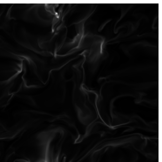
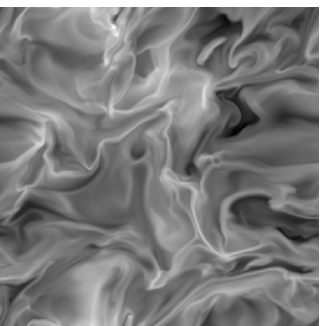
Figure 2 illustrates the structure of the density field in supersonic turbulence, modeled at a resolution of . The left hand side panel shows linear density. Due to the large density contrast, only a few shock sheets and filaments are visible. The right hand side panel shows logarithmic density, and illustrates the general presence of intermittent density structure over a range of scales and density levels.


The history of a fluid parcel in the real ISM might be as follows: It achieves initial, large kinetic energy by either being part of the ejecta from a supernova or, more likely, by being hit by the ejecta from a supernova. It becomes further compressed as the stream to which it belongs collides with other streams. As density increases cooling becomes significant, and the temperature decreases. The parcel may eventually end up as part of a molecular cloud. Inside the cloud, the process repeats itself, on successively smaller scales, creating in the end a shock core massive enough to form a star. More likely, though, the fluid parcel ends up in a structure too small to collapse by self-gravity, where it survives until being hit by the blast wave from another supernova, or the wind from a new-borne massive star.
3.3 Super-Alfvénic conditions
The proposal that magneto-hydrodynamic waves are main contributors to the velocity field in molecular clouds is now obsolete for several independent reasons. First, with the velocity field of molecular clouds part of a turbulent cascade there is no longer a problem to sustain the motions. Second, with the demonstrations that MHD-turbulence decays more or less as rapidly as hydrodynamic turbulence Biskamp+Muller00 ; MacLow_Puebla98 ; 1998ApSS.261..195M ; 1999ApJ…524..169M ; 1999ApJ…526..279P ; Stone+98 , the presumed ‘advantage’ of MHD-turbulence has gone away. Third, with observational and theoretical evidence that star formation takes place on a time scale not much longer than a crossing time 2000ApJ…530..277E the required life times of molecular clouds are much shorter than was assumed in earlier work.


The notion that the velocity field in molecular clouds is essentially Alfvén waves lead to the assumption that the kinetic and magnetic energy in molecular clouds are in near equipartition. Although inverting observations to obtain the magnetic field strength, density and velocity in the same structures is notoriously difficult (cf. the discussion in Section 4.1 of Goodman+Heiles94 ), equipartition remained a popular null-hypothesis.
With access to numerical simulations it is possible to use the more robust ‘forward analysis’ method, where synthetic diagnostics computed from the results of numerical simulations are compared directly with the corresponding observational diagnostics. Comparisons of extinction statistics, synthetic molecular lines, the antenna temperature – line width relation, and the statistical upper envelope relation between density and magnetic field strength (cf. Figs. 3–6) all lead to the same conclusion; models with equipartition between magnetic and kinetic energy are inconsistent with the observations while models where the kinetic energy dominates over the magnetic energy (super-Alfvénic models) are consistent with the observations 1997ApJ…474..730P ; 1998ApJ…504..300P ; 1999ApJ…525..318P ; 1999ApJ…526..279P .
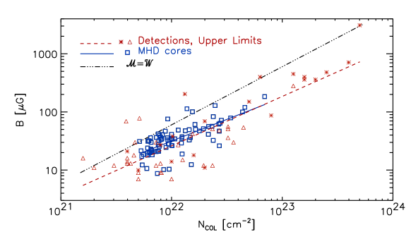
A direct illustration of the consistency of super-Alfvénic conditions with Zeeman observations of magnetic field strength is given in Fig. 7. Note that several cores with B in excess of 100 G are found, even though the average B in the simulation is only 2.4 G. This is a good example of the power of forward comparisons in situations with strong intermittency; it would be very difficult to recover the mean field strength, or the mean magnetic energy, directly from the observations, which sample only the very small fraction of the cloud volume filled by the densest regions. Further illustrations are given in Figs. 8–9, which show comparisons of velocity statistics with observations.
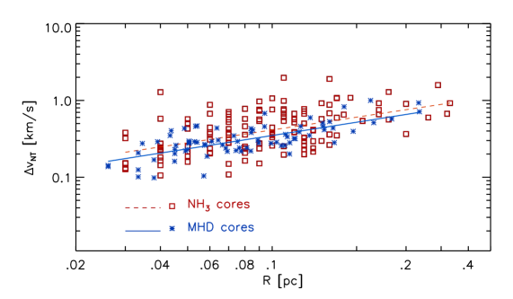
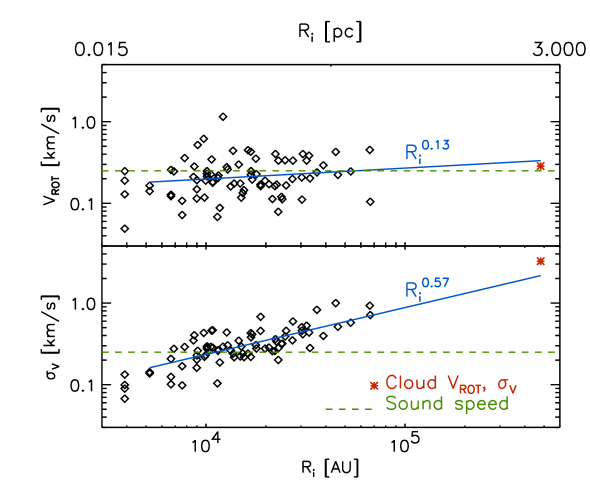
Figure 8 is a comparison of the correlation of non-thermal line width with size in NH3 cores from the compilation by Jijina, Myers & Adams 1999ApJS..125..161J and in cores selected from a simulation of supersonic and super-Alfvénic turbulence Padoan+Corsica02 . The least squares fit to the observational data yields the power law exponent and the fit to the data the exponent . Figure 9 shows the correlation of rotational velocity (upper panel) and internal velocity dispersion (lower panel) with size, for the numerical cores only. The rotational velocities are very low and of the order of the sound speed, as found in the observational data. In both panels of Fig. 9 the asterisk symbols that correspond to a size of almost 3 pc provide the values of rotational velocity and velocity dispersion computed over the whole simulated volume. Although the least squares fits are computed only for the cores, the values for the whole system are consistent with the fits.
3.4 The magnetic flux problem
A “magnetic flux problem” is often mentioned in this context. It is argued that since the average density of molecular clouds is at least 100 times larger than the average density in the galactic disk, and assuming magnetic flux freezing, the average magnetic field strength of molecular clouds should be much larger than the average galactic values of a few G. As demonstrated by Fig. 7 there is in fact no real problem – observations of core magnetic fields are completely consistent with predictions from models with average magnetic field strengths of a few G – there is at most a conceptual / perceived problem.
This conceptual problem has a straightforward solution, which, ironically, is most easily demonstrated by the equipartition model. It has been shown in many numerical works that supersonic turbulence, even with equipartition of kinetic and magnetic energy (the traditional model for molecular clouds) generates a complex density field, with very large contrast sheetlike and filamentary density structures. These density enhancements do not correspond to significant variations of the magnetic field strength in equipartition models, since in them strong compression can occur only along magnetic field lines. To the extent that turbulence on large scales (disk thickness) has approximate equipartition of kinetic and magnetic energy, molecular clouds can still easily form, as a consequence of compressions along magnetic field lines.
Once a cloud is formed by large scale equipartition turbulence, it has a mean magnetic field strength close to the galactic value, and its internal dynamics is super-Alfvénic, because of the much increased density. Equipartition on the large scale, therefore, is not a problem for the origin of super-Alfvénic clouds.
The argument applies recursively; should the super-Alfvénic cloud by chance create a region with local equipartition, further increase of the density is still possible, by inflow of mass along magnetic field lines. One sees the statistical outcome of this in the B-n relation (Fig. 6); for any given density there is a wide distribution of magnetic field strengths, up to an upper envelope given by approximate equipartition.
Inflow along magnetic field lines is also likely to occur in the phase when gravitation has taken over, after local cores are formed along filaments and in corrugated sheets. In that situation the magnetic field has already been compressed, and is oriented predominantly along the same filaments and sheets that also contain abundant mass at high density.
3.5 Gravitationally bound and unbound clouds
The scenario where star formation takes place in essentially a crossing time 2000ApJ…530..277E also alleviates earlier concerns about how to support molecular clouds against gravitational collapse. The gravitational binding energy of molecular clouds is often comparable to their turbulent kinetic energy, and hence quite a bit larger than their thermal energy 1981MNRAS.194..809L ; 1992A&A…257..715F . This raised the question of the support of the clouds against gravitational collapse. Could the turbulent velocities be translated into a turbulent pressure that was able to support the clouds against collapse 1987A&A…172..293B ; 1992JFM…245….1B ; 1995A&A…303..204V ; 2000ApJ…535..887K ? Or did the solution lie in the observed, strong fragmentation of the medium 1982ApJ…258L..29S ; 1995MNRAS.277..377P ?
In the ‘turbulent fragmentation & star formation in a crossing time’ paradigm it is natural to find some molecular clouds with roughly virial mass, as well as some with substantially less than virial mass, while there are essentially none with much larger than virial mass (cf. Fig. 7 of 1992A&A…257..715F ). Turbulent fragmentation creates clouds, initially without regard to gravity. Some of the clouds that are produced are gravitationally unbound (but may contain sub-structures that are gravitationally bound). Some other clouds are massive enough to be gravitationally bound (at least until their first supernovae blow out a major part of the cloud gas). Clouds that are created with a mass larger than virial start to collapse, which increases the velocity dispersion of their sub-structures until they appear to be essentially virial.
The latter case represents the most direct and simple mechanism by which turbulence prevents global collapse of molecular clouds; i.e., through fragmentation rather than through “turbulent pressure”. The mechanism may be illustrated by considering that extreme intermittency caused by strongly supersonic turbulence and cooling could create conditions where individual density maxima move in essentially ballistic orbits relative to one another 1982ApJ…258L..29S . Even under less extreme conditions intermittency may cause individual density maxima to collapse, while the cloud as such does not 1995MNRAS.277..377P ; 1997MNRAS.288..145P ; 2000ApJ…535..887K ; 2001ApJ…547..280H .
3.6 Power laws and equipartition
As mentioned above, even highly supersonic turbulence is characterized by power laws Boldyrev+1 ; Boldyrev+2 . However, because of the strong intermittency of density and its correlation with the velocity field, the spectrum of kinetic energy is not the same as the power spectrum of velocity.
It is appropriate to define the spectrum of kinetic energy as the power spectrum of , since the sum of squares of its Fourier components is equal to the kinetic energy. Empirically, from numerical simulations, one finds that the spectrum of kinetic energy is quite a bit more shallow than the power spectrum of velocity. The latter has a power exponent consistent with the theoretical expectation Boldyrev+1 . The former has a power exponent .
The power spectrum of the magnetic field is approximately parallel to that of velocity in the high-k part of the inertial range, and hence the spectrum of magnetic energy is steeper than the spectrum of kinetic energy. This may appear strange, at first. Why would the magnetic field have a power spectrum similar to that of velocity, when magnetic energy, , is measured in the same units as kinetic energy and not in the units of velocity power ? A possible explanation is that is weighted more towards the kinetic energy of the bulk of the volume. Assuming a log-normal PDF of density, with a dispersion of linear density 1999intu.conf..218N
| (3) |
where , the most common density is
| (4) |
which is smaller than the average density . Thus, if the magnetic energy is in equipartition with the kinetic energy at those densities, rather than at the higher densities towards which the average kinetic energy is weighted, this would explain both why the spectrum of is similar to that of and why the average magnetic energy is below equipartition with the kinetic energy.
With a difference in the power law exponents a gap develops from the (observed) equipartition at large scales ( 100 pc). A power law index difference of 0.65 implies at pc scales, which is consistent with the forward analysis of numerical simulations 1999ApJ…526..279P .
Note that the discussion above is complementary to the one at the end of Sect. 3.3 – both views are helpful for understanding why small scale ISM motions are super-Alfvénic.
4 A new analytical theory of supersonic turbulence
Due to the complexity of the Navier-Stokes equations, mathematical work on turbulence is often inspired by experimental and observational measurements. Since geophysical and laboratory flows are predominantly incompressible, turbulence studies have been limited almost entirely to incompressible flows (or to infinitely compressible ones, described by the Burgers equation). Little attention has been paid in the past to highly compressible, or super-sonic turbulence.
Turbulent flows are traditionally described statistically by the structure functions of their velocity field Frisch95 . The structure functions are defined as
| (5) |
where is the component of the velocity field perpendicular (transversal structure functions) or parallel (longitudinal structure functions) to the vector . In the inertial interval the structure functions obey scaling laws and the exponent can be determined. The power spectrum of the velocity is the Fourier transform of the second order structure function, and may be expressed as .
One may think that the study of high order structure functions is interesting only for testing models of intermittency in turbulent flows, and not very useful in the context of ISM turbulence and star formation. Actually, the intermittent nature of turbulence is crucial in modeling the process of star formation driven by turbulent fragmentation. Stars are formed in the densest regions of turbulent flows. These regions contain only a few percent of the total mass and fill an almost insignificant fraction of the total volume of a star forming cloud. High order moments defining the tails of statistical distributions of velocity and density are therefore very important in the process of star formation. Furthermore, low order density structure functions, which are obviously important to describe basic properties of turbulent fragmentation, can be shown to depend on velocity structure functions of very high order Boldyrev+2 .
The scaling of the velocity structure functions in incompressible turbulence is best described by the She-Leveque formula SL94 ,
| (6) |
The scaling exponents are computed relative to the third order, , because according to the concept of extended self-similarity Benzi+93 ; Dubrulle94 the relative exponents are universal and better defined than the absolute ones.
Boldyrev Boldyrev has proposed an extension of the She-Leveque’s formalism SL94 to the case of supersonic turbulence. Based on the physical interpretation of (6) by Dubrulle Dubrulle94 , a fundamental parameter in the derivation of the velocity structure functions is the Hausdorff dimension of the support of the most singular dissipative structures in the turbulent flow. In incompressible turbulence the most dissipative structures are organized in filaments along coherent vortex tubes with Hausdorff dimension , while in supersonic turbulence dissipation occurs predominantly in sheet-like shocks, with Hausdorff dimension . The new velocity structure function scaling proposed by Boldyrev Boldyrev for supersonic turbulence is
| (7) |
This velocity scaling has been found to provide a very accurate prediction for numerical simulations of supersonic and super-Alfvénic turbulence Boldyrev+1 , and has been used to infer the structure of the density distribution in turbulent clouds Boldyrev+2 .
5 Star formation and the Initial Mass Function
At least three unrelated ways of explaining the process of star formation and the origin of the stellar initial mass function (IMF) may be found in the literature: i) Ambipolar drift contraction of sub-critical cores 1987ARA&A..25…23S ; 1996ApJ…464..256A ; ii) opacity-limited gravitational fragmentation 1953ApJ…118..513H ; 1963ApJ…138.1050G ; 1972PASJ…24…87Y ; 1976SvA….19..403S ; 1976MNRAS.176..367L ; 1976MNRAS.176..483R ; 1977ApJ…214..718S ; 1977ApJ…214..152S ; 1985ApJ…295..521Y ; and iii) turbulent fragmentation 1971ApJ…169..289A ; 1981MNRAS.194..809L ; 1982ApJ…258L..29S ; 1993ApJ…419L..29E ; 1994ApJ…423..681V ; 1995MNRAS.277..377P ; 2001ApJ…553..227P ; Padoan+Nordlund-IMF .
The first type of models rely on the assumption that both protostellar cores and their parent clouds are long lived systems in near equilibrium, supported against their gravitational collapse by magnetic field pressure. As discussed above, this assumption has been proven incorrect based on observational data and is inconsistent with the turbulent nature of star-forming clouds 1999ApJ…526..279P ; 2000ApJ…530..277E ; 2001ApJ…562..852H ; 2001ApJ…553..227P . Furthermore, these type of models do not address the problem of the formation of massive stars or brown dwarfs, and have traditionally focused more on the evolution of individual protostars, without providing a self-consistent picture for the origin of the initial conditions.
The second type of models is also inconsistent with the properties of star-forming clouds, because it applies the concept of gravitational fragmentation to the large scale, in the attempt of modeling the formation of a whole stellar population. The concept of gravitational instability is based on a comparison between the gas thermal and gravitational energies to define the smallest unstable mass, or Jeans’ mass. However, star-forming clouds, as any region of the cold ISM above a scale of approximately 0.1 pc, contain a kinetic energy of turbulence that is much larger (typically 100 times larger) than their thermal energy, making the comparison of thermal and gravitational energies irrelevant on the large scale. Attempts to redefine the Jeans’ mass Chandrasekhar58 ; 1971ApJ…169..289A assuming that turbulence can provide pressure support against the gravitational collapse are flawed, because they miss the basic point that supersonic turbulence is actually fragmenting the gas. The main effect of the large kinetic energy of turbulence, relative to the thermal energy, is that the gas density and velocity fields in star-forming regions are highly non-linear, against the assumption of the gravitational instability model. In other words, clouds are already fragmented by turbulence, quite independent of their self-gravity.
The third type of models, which we refer to as turbulent fragmentation models, focus on the importance of the observed supersonic turbulence in molecular clouds and are therefore consistent with the large scale dynamics of star-forming regions. The idea of star formation driven by supersonic turbulence was proposed twenty years ago by Larson 1981MNRAS.194..809L , but has become popular only in the last few years, thanks to the progress of numerical simulations of supersonic magneto-hydrodynamic (MHD) turbulence.
According to the model of turbulent fragmentation, protostellar cores are formed from gas compressed by shocks in the supersonic turbulent flow 2001ApJ…553..227P . While scale-free turbulence generates a power law mass distribution down to very small masses, only cores with a gravitational binding energy in excess of their magnetic and thermal energy can collapse. The shape of the stellar IMF is then a power law for large masses, since the majority of large cores are larger than their Jeans’ mass. At smaller masses, the IMF flattens and then turns around according to the probability of small cores to be dense enough to collapse, which is determined by the PDF of gas density.
5.1 The Initial Mass Function
The mass distribution of dense cores formed in a supersonic turbulent flow follows from a number of properties of such flows Padoan+Nordlund-IMF : i) The power spectrum of the turbulence is a power law; ii) the dynamics on scales covered by the power law is approximately selfsimilar; iii) the typical size of a dense core scales as the thickness of the postshock gas; iv) the relevant shock jump conditions are those of MHD shocks.
These properties are to a considerable extent already verified by numerical simulations, which also produce corresponding numerical IMFs Padoan+Corsica02 , but for the purpose of deriving a theoretical IMF one may just adopt them as assumptions Padoan+Nordlund-IMF .
The second assumption, about approximate selfsimilarity, is a crucial one. Since velocity amplitudes do depend on scale (by the first assumption and by Larson’s relation) it is not an exact property. Nevertheless, since these flows are supersonic they follow essentially inertial paths in a large fraction of space (upstream of shocks). The thickness and density of the downstream, shocked gas does depend on the Mach number, and hence on the scale, but the filling factor of the shocked gas is quite small and does not disturb the overall selfsimilarity much.
The distribution of cores that form in the shocked, downstream gas may be regarded as a distribution over linear sizes of the upstream flows out of which they formed. By the assumption of approximate selfsimilarity the number of such regions per unit log scales as . The upstream (Alfvénic) Mach number is denoted and is assumed to scale as , where is related to the power spectrum index .
The typical mass of the cores that form in the shocked gas scales as , where (from the MHD shock jump conditions) is the thickness of the postshock gas, is its density, where is the upstream mass density (similar to the mean density). The typical core mass is thus
| (8) |
which leads to the following expression for the mass distribution of dense cores:
| (9) |
If the power spectral index is consistent with the observed velocity dispersion-size Larson relation 1981MNRAS.194..809L and with the numerical and analytical results Boldyrev ; Boldyrev+1 , then and the mass distribution is
| (10) |
which is almost identical to the Salpeter stellar IMF 1955ApJ…121..161S .


If is defined as the scale of a molecular cloud, with average mass density and Alfvénic Mach number , the mass of the largest cores formed by turbulent fragmentation is estimated to be
| (11) |
In MCs with mass M⊙ and Mach number , M⊙.
While the majority of massive cores are larger than their Jeans’ mass, , the probability that small cores are dense enough to collapse is determined by the PDF of the density of the cores, which is approximately Log-Normal. Even very small (sub-stellar) cores have a finite chance to be dense enough to collapse. If is the Jeans’ mass distribution obtained from the PDF of gas density 1997MNRAS.288..145P , the fraction of cores of mass with gravitational energy in excess of their thermal energy is given by the integral of from 0 to . The mass distribution of collapsing cores is therefore
| (12) |
The mass distribution is plotted in Fig. 10, for . In the top panel the mass distribution is shown for three different values of the largest turbulent scale , assuming Larson type relations 1981MNRAS.194..809L to rescale the average gas density, , and the rms Mach number, , as a function of size, . The mass distribution is a power law, determined by the power spectrum of turbulence, for masses larger than approximately 1 m⊙. At smaller masses the mass distribution flattens, reaches a maximum at a fraction of a solar mass, and then decreases with decreasing stellar mass. The mass distribution peaks at approximately m⊙ for the values , cm-3, K and , typical of nearby molecular clouds. Collapsing sub-stellar masses are found, thanks to the intermittent density distribution in the turbulent flow. This provides a natural explanation for the origin of brown dwarfs.
Note that the power law shape of the IMF for mass values larger than about 1 m⊙ is not affected by the average physical properties of the system. On the other hand the abundance of brown dwarfs is very sensitive to the average gas density and the rms Mach number of the flow. The middle and bottom panels of Fig. 10 show the dependence of the mass distribution on the rms Mach number of the flow and on the average gas density respectively. One can see in the middle panel that for an average gas density of cm-3 and an rms Mach number , typical of a molecular cloud complex such as Taurus, brown dwarfs are very rare, while for the same average gas density and an rms Mach number , typical of a molecular cloud complex such as Orion (the density may be even larger), brown dwarfs are very abundant (even more abundant if the IMF were plotted in units of linear mass interval). This prediction is in fact unambiguously confirmed by the observations 2000ApJ…544.1044L .
The thermal Jeans’ mass is a more strict condition for collapse than the magnetic critical mass. The magnetic critical mass depends on the core morphology in relation to the magnetic field geometry and strength. The latter correlates with the gas density with a very large scatter 1999ApJ…526..279P . It is possible therefore that magnetic pressure support against the gravitational collapse limits the efficiency of star formation, while its effect on the shape of the mass distribution is of secondary importance.
Observations show that the stellar IMF is a power law above 1–2 m⊙, with exponent around the Salpeter value , roughly independent of environment Elmegreen_rev98 ; Elmegreen_rev2000 , gradually flattens at smaller masses, and peaks at approximately 0.2–0.6 m⊙ 1997AJ….113.1733H ; 1998A&A…336..490B ; 1999ApJ…525..440L ; 1999ApJ…525..466L ; 2000ApJ…540.1016L ; 2000ApJ…544.1044L . The shape of the IMF below 1–2 m⊙, and particularly the relative abundance of brown dwarfs, may depend on the physical environment 2000ApJ…544.1044L . These observational results are all consistent with our theoretical IMF.
It has been argued that only a small fraction of the mass of each collapsing core may end up into the final star, due to mass loss in protostellar winds, with a major effect on the stellar IMF. However, stellar winds could be important for the origin of the stellar IMF only if the ratio of initial core mass to final stellar mass were comparable to the total mass range for stars (, from M⊙ to M⊙), as pointed out by Elmegreen 1999ApJ…522..915E . This is highly unlikely, because i) the correct slope and mass range of the IMF is already achieved by turbulent fragmentation alone and ii) observational results indicate that the mass distribution of prestellar cores is indistinguishable from the stellar IMF 1998A&A…336..150M ; 2001A&A…372L..41M ; 1998ApJ…508L..91T ; 1999sf99.proc..153O , as predicted in earlier work on turbulent fragmentation and the origin of the stellar IMF 1995MNRAS.277..377P .
5.2 Mass distribution of prestellar cores in numerical simulations
The mass distribution of prestellar cores may be measured directly in numerical simulations of supersonic turbulence. With a mesh of 2503 computational cells, and assuming a size of the simulated region of a few pc, it is not possible to follow numerically the gravitational collapse of individual protostellar cores. However, dense cores at the verge of collapse can be selected in numerical simulations by an appropriate clumpfind algorithm. Such an algorithm should scan all density levels and recognize when a large core is fragmented into smaller and denser ones, in which case the large core should not be counted. Cores should also be excluded if their gravitational energy is not large enough to overcome thermal and magnetic support against the collapse, since only collapsing cores should be selected.

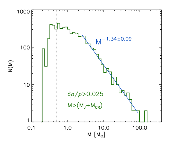
A mass distribution of collapsing cores, derived from the density distribution in a numerical simulation is shown in Fig. 11. The computational box with 1283 cells has been scaled to two scale ranges, suitable for sampling cores in the intervals 0.2–2 M⊙ and 2–100 M⊙, respectively. The mass distribution above 1 M⊙ is a power law consistent with our analytical result and with the observations. Below 1 M⊙ the histogram flattens and then turns around at approximately 0.3 M⊙, also consistent with the analytical theory and the observations. The cut-off at 0.2 M⊙ is due to the finite numerical resolution; the grid size, rms Mach number, and mean density together impose a limitation on the mass of collapsing cores.
Stretching the mass interval of sampled cores further into the brown dwarf regime requires larger numerical resolution. Figure 12 shows the mass distribution of collapsing cores derived from two snapshots of a 2503 simulation. The average gas density has been scaled to 500 cm-3 and the size of the computational box to 10 pc. These values have been chosen to be able to select cores in a range of masses from a sub-stellar mass to approximately 10 M⊙. With this particular values of average gas density and size of the computational box, the smallest mass that can be achieved numerically is 0.057 M⊙. Brown dwarfs masses ( M⊙) are therefore included. With an even larger numerical mesh, or assuming a larger average density (and a smaller size), even smaller masses would be selected. Turbulent fragmentation thus provides a natural explanation for the origin of brown dwarfs. This was found from the analytical model of the IMF presented above and is here confirmed from the numerical mass distribution.
Observed star-forming clouds appear very filamentary, as the projected density field of supersonic turbulent flows. We have performed accurate comparisons of statistical properties of turbulent flows with observational data, by computing synthetic spectral maps of molecular transitions 1998ApJ…504..300P ; 1999ApJ…525..318P ; 2001ApJ…553..227P . The synthetic spectral maps are obtained by computing the non-LTE radiative transfer problem using the density and velocity fields of the MHD simulations. We have shown that fundamental statistical properties of supersonic turbulence are unambiguously found in the observational data of star-forming clouds 2001ApJ…553..227P .
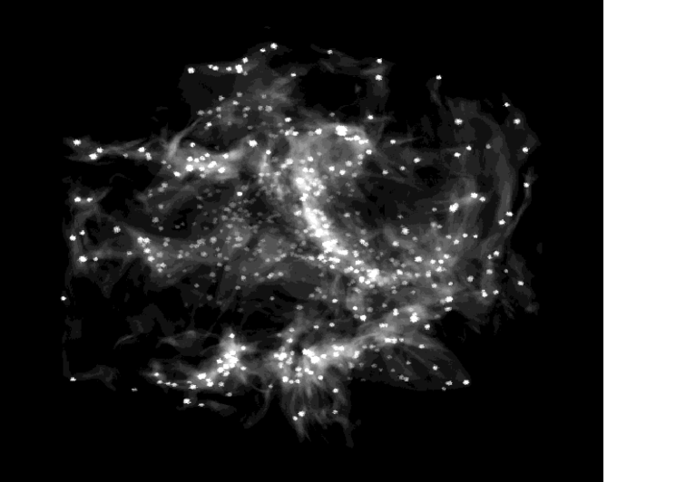
In star-forming clouds, prestellar cores and young stars tend to concentrate in the densest filaments and cores. Since filaments and cores of the same nature are found in the numerical simulations, it is interesting to visualize the position of the collapsing cores selected numerically, relative to the gas density distribution. In Fig. 13 a voxel projection of the density field is shown, where all the numerically selected cores have been highlighted as bright spheres. The size and brightness is a function of the core mass. The brightness is also a function of the optical depth of the gas between the observer and the stars, to mimic the effect of dust extinction. Figure 13 shows beautiful filamentary structure in both the gas and the stellar distribution, very reminiscent of observed star-forming regions. It is quite amazing that a numerical simulation of randomly driven supersonic and super-Alfvénic turbulence with periodic boundary conditions is able to produce at the same time i) density structures morphologically and statistically consistent with the observations; ii) prestellar cores correlated with the gas distribution in a way qualitatively similar to the observations and with a value of magnetic field strength typically observed; iii) a mass distribution of the same prestellar cores that agrees with the observed stellar (and prestellar cores) mass distribution over the whole range of stellar masses, from brown dwarfs to massive stars; and iv) a star formation efficiency consistent with that in observed molecular clouds of only a few percent per large scale dynamical time.
6 Conclusions
The main conclusion from the preceding sections is that the statistics of star formation is primarily controlled by supersonic turbulence, rather than by gravity. Star formation takes place in cold molecular clouds, which are part of a turbulent cascade in the interstellar medium. The ultimate energy input to the cascade comes from supernovae, with a possibly significant contribution from local variations of the galactic rotation curve (density waves). The clouds owe their existence to random convergence of the interstellar medium velocity field, which creates local density enhancements over a range of scales. The internal, supersonic and super-Alfvénic velocity field in molecular clouds is responsible for their fragmentation, thus preventing global collapse but triggering local collapse at the many local density maxima whose mass exceeds the local Jeans’ mass. Such prestellar cores are formed as sheet corrugations and filamentary density enhancements, and are taken over by self-gravity only after they have been shaped by the turbulence.
The velocity field of the cascade is dominated by power in solenoidal (shearing) motions, even though it is supersonic and super-Alfvénic. Its spectrum of kinetic energy is less steep than its velocity and magnetic field power spectra, which explains how conditions can be super-Alfvénic on small (molecular cloud) scales, even though there is rough equipartition between magnetic and kinetic energy density on large (disk thickness) scales.
A Salpeter like IMF is the result of the near-self-similar, power law nature of turbulence in molecular clouds, in combination with density jump amplitudes determined by MHD-shock jump conditions.
Star formation (at least in our galaxy) bites its own tail; it is driven by supernovae and at the same time the birth of massive stars gives rise to new supernovae that re-enforce the driving. External sources of turbulence, such as kinetic energy from galaxy collisions and merging may be the primary driving agent in star-burst galaxies.
Different physical conditions (primarily higher temperatures and lower metal abundances) in the Early Universe would lead to higher mass at the low-mass cut-off, and a much weaker magnetic field would lead to a steeper IMF slope.
Acknowledgments
The work of ÅN was supported by a grant from the Danish Natural Science Research Council, and in part by the Danish National Research Foundation, through its establishment of the Theoretical Astrophysics Center. The work of PP was in part performed while PP held a National Research Council Associateship Award at the Jet Propulsion Laboratory, California Institute of Technology.
References
- (1) Adams, F. C. and Fatuzzo, M.: Astrophys. J. 464, 256 (1996)
- (2) Arny, T.: Astrophys. J. 169, 289 (1971)
- (3) Arons, J. and Max, C. E.: Astrophys. J. 196, L77 (1975)
- (4) de Avillez, M. A.: MNRAS 315, 479 (2000)
- (5) Ballesteros-Paredes, J., Vázquez-Semadeni, E., and Scalo, J.: Astrophys. J. 515, 286 (1999)
- (6) Ballesteros-Paredes, J., Hartmann, L., and Vázquez-Semadeni, E.: Astrophys. J. 527, 285 (1999)
- (7) Benzi, R., Ciliberto, S., Tripiccione, R., Baudet, C., Massaioli, F., and Succi, S.: Phys. Rev. E 48, 29 (1993)
- (8) Biskamp, D., and Muller, W. C.: Physics of Plasmas, 7 (12), 4889 (2000)
- (9) Boldyrev S., Astrophys. J. 569, No. 2, April 20; astro-ph/0108300 (2002)
- (10) Boldyrev S.: private communication (2002)
- (11) Boldyrev, S., Nordlund, Å., and Padoan, P.: Astrophys. J. 573, (2002)
- (12) Boldyrev, S., Nordlund, Å., and Padoan, P.: Supersonic turbulence and structure of interstellar molecular clouds, submitted to Phys. Rev. Lett., astro-ph/0203452 (2002)
- (13) Bonazzola, S., Heyvaerts, J., Falgarone, E., Perault, M., and Puget, J. L.: Astron. Astrophys. 172, 293 (1987)
- (14) Bonazzola, S., Perault, M., Puget, J. L., Heyvaerts, J., Falgarone, E., and Panis, J. F.: Journal of Fluid Mechanics 245, 1 (1992)
- (15) Boulares, A. and Cox, D. P.: Astrophys. J. 365, 544 (1990)
- (16) Bourke, T. L., Myers, P. C., Robinson, G., and Hyland, A. R.: Astrophys. J. 554, 916 (2001)
- (17) Bouvier, J., Stauffer, J. R., Martin, E. L., Barrado y Navascues, D., Wallace, B., and Bejar, V. J. S.: Astron. Astrophys. 336, 490 (1998)
- (18) Chandrasekhar, S.: Proc. R. Soc. London, Ser. A, 246, 301 (1958)
- (19) Dubrulle, B.: Phys. Rev. Lett. 73, 959 (1994)
- (20) Efstathiou, G.: MNRAS 317, 697 (2000)
- (21) Elmegreen, B. G.: Astrophys. J. 419, L29 (1993)
- (22) Elmegreen, B. G.: in M. Livio (ed.), Unsolved Problems in Stellar Evolution, Cambridge University Press, p. 59 (1998)
- (23) Elmegreen, B. G.: Astrophys. J. 522, 915 (1999)
- (24) Elmegreen, B. G.: in T. Montmerle and Ph. André (eds.) From Darkness to Light, ASP Conference Series (2002)
- (25) Elmegreen, B. G.: Astrophys. J. 530, 277 (2000)
- (26) Falgarone, E. and T. G. Phillips: Astrophys. J. 359, 344 (1990)
- (27) Falgarone, E., J.-L. Puget, and M. Perault: Astron. Astrophys. 257, 715 (1992)
- (28) Frisch, U.: Turbulence, Cambridge University Press (1995)
- (29) Gaustad, J. E.: Astrophys. J. 138, 1050 (1963)
- (30) Goodman, A., and Heiles, C.: Astrophys. J. 424, 208 (1994)
- (31) Goodman, A. A., Barranco, J. A., Wilner, D. J., and Heyer, M. H.: Astrophysical Journal 504, 223 (1998)
- (32) Gudiksen, B. V.: PhD thesis, Niels Bohr Institute for Astronomy, Physics, and Geophysics, University of Copenhagen (1999)
- (33) Hartmann, L., Ballesteros-Paredes, J., and Bergin, E. A.: Astrophys. J. 562, 852 (2001)
- (34) Heitsch, F., Mac Low, M., and Klessen, R. S.: Astrophys. J. 547, 280 (2001)
- (35) Hillenbrand, L. A.: Astronomical Journal 113, 1733 (1997)
- (36) Hoyle, F.: Astrophys. J. 118, 513 (1953)
- (37) Jijina, J., Myers, P. C., and Adams, F. C.: Astrophysical Journal Supplement Series 125, 161 (1999)
- (38) Klessen, R. S., Heitsch, F., and Mac Low, M.: Astrophys. J. 535, 887 (2000)
- (39) Kolmogorov, A. N.: Dokl. Akad. Nauk. SSSR, 30, 301 (1941)
- (40) Korpi, M. J., Brandenburg, A., Shukurov, A., Tuominen, I., and Nordlund, Å.: Astrophys. J. 514, L99 (1999)
- (41) Lada, C. J., Lada, E. A., Clemens, D. P., Bally, J.: Astrophys. J., 429, 694 (1994)
- (42) Larson, R. B.: MNRAS 186, 479 (1979)
- (43) Larson, R. B.: MNRAS 194, 809 (1981)
- (44) Larson, R. B.: MNRAS 200, 159 (1982)
- (45) Low, C. and Lynden-Bell, D.: MNRAS 176, 367 (1976)
- (46) Luhman, K. L.: Astrophys. J. 525, 466 (1999)
- (47) Luhman, K. L.: Astrophys. J. 544, 1044 (2000)
- (48) Luhman, K. L. and Rieke, G. H.: Astrophys. J. 525, 440 (1999)
- (49) Luhman, K. L., Rieke, G. H., Young, E. T., Cotera, A. S., Chen, H., Rieke, M. J., Schneider, G., and Thompson, R. I.: Astrophys. J. 540, 1016 (2000)
- (50) Mac Low, M.-M.: in J. Franco, A. Carramiñana (eds.), Interstellar Turbulence, Cambridge University Press (1999)
- (51) Mac Low, M.-M.: Astrophys. J. 524, 169 (1999)
- (52) Mac Low, M., Smith, M. D., Klessen, R. S., and Burkert, A.: jtitleThe Decay of Supersonic and Super-Alfvenic Turbulence in Star-Forming Clouds Astrophysics and Space Science 261, 195 (1998)
- (53) Motte, F., Andre, P., and Neri, R.: Astron. Astrophys. 336, 150 (1998)
- (54) Motte, F., André, P., Ward-Thompson, D., and Bontemps, S.: Astron. Astrophys. 372, L41 (2001)
- (55) Nordlund, Å. and Padoan, P.: in J. Franco, A. Carramiñana (eds.), Interstellar Turbulence, Cambridge University Press, p. 218 (1999)
- (56) Onishi, T., Mizuno, A., Kawamura, A., and Fukui, Y.: in T. Nakamoto (ed.) Proceedings of Star Formation 1999, Nobeyama Radio Observatory, p. 153 (1999)
- (57) Ossenkopf, V., and Mac Low, M.-M.: Turbulent Velocity Structure in Molecular Clouds submitted to Astron. Astrophys., astro-ph/0012247 (2002)
- (58) Ostriker, E. C., Stone, J. M., and Gammie, C. F.: Astrophys. J. 546, 980 (2001)
- (59) Padoan, P.: MNRAS 277, 377 (1995)
- (60) Padoan, P., Jones, B. J. T., and Nordlund, Å.: Astrophys. J. 474, 730 (1997)
- (61) Padoan, P., Nordlund, Å., and Jones, B. J. T.: MNRAS 288, 145 (1997)
- (62) Padoan, P., Juvela, M., Bally, J., and Nordlund, A.: Astrophys. J. 504, 300 (1998)
- (63) Padoan, P., Bally, J., Billawala, Y., Juvela, M., and Nordlund, Å.: Astrophys. J. 525, 318 (1999)
- (64) Padoan, P. and Nordlund, Å.: Astrophys. J. 526, 279 (1999)
- (65) Padoan, P., Juvela, M., Goodman, A. A., and Nordlund, Å.: Astrophys. J. 553, 227 (2001)
- (66) Padoan, P., and Nordlund, Å.: The Stellar IMF from Turbulent Fragmentation, submitted to Astrophys. J., astro-ph/0011465 (2002)
- (67) Padoan, P., Nordlund, Å., Rögnvaldsson, Ö. E., and Goodman, A.: in T. Montmerle and Ph. André (eds.) From Darkness to Light, ASP Conference Series (2002)
- (68) Padoan, P., Nordlund, Å., Rögnvaldsson, Ö. E., and Goodman, A.: submitted to Astrophys. J., astro-ph/0011229 (2002)
- (69) Passot, T., Vazquez-Semadeni, E., and Pouquet, A.: Astrophys. J. 455, 536 (1995)
- (70) Passot, T., and Vazquez-Semadeni, E.: Phys. Rev. E 58, 4501 (1998)
- (71) Rees, M. J.: MNRAS 176, 483 (1976)
- (72) Salpeter, E. E.: Astrophys. J. 121, 161 (1955)
- (73) Scalo, J. M. and Pumphrey, W. A.: Astrophys. J. 258, L29 (1982)
- (74) Scalo, J., Vazquez-Semadeni, E., Chappell, D., and Passot, T.: Astrophys. J. 504, 835 (1998)
- (75) She, Z.-S., and Lévêque, E.: Phys. Rev. Lett. 72 336 (1994)
- (76) Shu, F. H., Adams, F. C., and Lizano, S.: Annual Review of Astronomy and Astrophysics 25, 23 (1987)
- (77) Silk, J.: Astrophys. J. 214, 152 (1977)
- (78) Silk, J.: Astrophys. J. 214, 718 (1977)
- (79) Stone, J. M., Ostriker, E. C., Gammie, C. F.: Astophys. J. Lett. 508, L99 (1998)
- (80) Struck, C., and Smith, D. C.: Astrophys. J. 527, 673 (1999)
- (81) Suchkov, A. A., and Shchekinov, I. A.: Soviet Astronomy 19, 403 (1976)
- (82) Testi, L., and Sargent, A. I.: Astrophys. J. 508, L91 (1998)
- (83) Vazquez-Semadeni, E.: Astrophys. J. 423, 681 (1994)
- (84) Vazquez-Semadeni, E. and Gazol, A.: Astron. Astrophys. 303, 204 (1995)
- (85) Vazquez-Semadeni, E., Passot, T., and Pouquet, A.: Astrophys. J. 441, 702 (1995)
- (86) Yoneyama, T.: Publications of the Astronomical Society of Japan 24, 87 (1972)
- (87) Yoshii, Y. and Saio, H.: Astrophys. J. 295, 521 (1985)
- (88) Zweibel, E. G. and Josafatsson, K.: Astrophys. J. 270, 511 (1983)