Natural Inflation, Planck Scale Physics
and Oscillating Primordial Spectrum

Abstract

In the “natural inflation” model, the inflaton potential is periodic. We show that Planck scale physics may induce corrections to the inflaton potential, which is also periodic with a greater frequency. Such high frequency corrections produce oscillating features in the primordial fluctuation power spectrum, which are not entirely excluded by the current observations and may be detectable in high precision data of cosmic microwave background (CMB) anisotropy and large scale structure (LSS) observations.

I Introduction

In the past decade, inflation theory has successfully passed several non-trivial tests. In particular, recent cosmic microwave background (CMB) observations show that the spatial geometry of the observable Universe is very close to flat de Bernardis00 ; Lange00 ; Hanany00 ; Balbi00 ; Jaffe00 , just as inflation theory predicts. Inflation theory also offers an elegant way of generating the primordial fluctuations which seed the formation of galaxies and large scale structures (LSS)(see e.g., Ref. Lyth-Riotto99 and references therein). In particular, slow-roll inflation models predict that the perturbations are adiabatic, gaussian, and nearly scale-invariant (i.e with a power index $n_{s}\simeq 1$). It has long been known that these predictions are also in broad agreement with the observed properties of large scale structures and CMB anisotropy, although at present the data is still not very restrictive Wang01 : $n_{s}=0.91^{+0.15}_{-0.07}$.

This general success of inflation theory brings up the hope of extracting even more detailed information of the inflaton potentialLyth-Riotto99 ; Lidsey97 from high quality observational data. There are two complementary approaches to this problem. In the first approach, one tries a model-independent (subject to some standard assumptions) reconstruction of the primordial power spectrum, then the inflaton potential from the data Hannestad01 ; MSY01 ; Wang-Mathews02 . Alternatively, one can look for specific features in the power spectrum and study their observational consequences. In particular, there have been many investigations on inflationary models with broken scale invarianceKLS85 ; Starobinsky92 ; ARS97 ; LPS98 ; Chung00 ; WK00 ; L00 . Such features have been invoked to explain the tentatively observed feature at $k\sim 0.05Mpc^{-1}$GSZ00 ; HHV01 ; BGSS00 ; GH01 , or even to solve the small scale problem of the CDM model KL00 .

In the present work, we consider a new type of feature, periodic in the primordial power spectrum. This type of feature is interesting from both a theoretical and phenomenological point of view. Theoretically, if discovered, it gives a strong hint on the nature of the inflaton field. Phenomenologically, it might change the position, shape or even the number of acoustic peaks in the CMB power spectrum.

This paper is organized as follows: in Sec. II, we describe our model, and show how this type of feature could arise from Planck scale physics by constructing a toy model. Our toy model, which is based on the “natural inflation” model, is by no means the only possibility, but in this context it is particularly easy to see how this might happen. In Sec. III we derive the power spectrum in this model, and then consider how it would affect CMB and large scale structure in Sec. IV. The final section, Sec.V is on the summary and discussions of our results.

II The Model

In addition to phenomenological success, a compelling inflation model should also be based on plausible particle physics. To be in agreement with observations, the inflaton potential must be very flat. Since the radiative corrections to a scalar field mass are quadratically divergent, some physical mechanism, e.g., a symmetry is required to maintain the flatness of the potential, unless we want to accept ad hoc fine tuning.

For the natural inflation model FFO90 , several possible physical mechanisms ABFFO93 are available for producing a inflaton potential of the form

$$V(\phi)=\Lambda^{4}\left[1\pm\cos(\phi/f)\right].$$ (1)

Customarily, the positive sign is taken, with identical results for the negative sign. If $\Lambda\sim 10^{16}\,{\rm GeV}$ and $f\sim 10^{19}\,{\rm GeV}$, which are the grand unification scale and Planck scale respectively, a successful inflation model could be obtained, with the correct quantum fluctuation amplitudes MT01 .

In this paper we extend the natural inflation model above and include a term in the potential in Eq.(1) which is also periodic but with greater frequency:

$$V_{planck}(\phi)=\delta\Lambda^{4}\cos(N\phi/f+\theta).$$ (2)

We will argue below that this term may come from the Planck scale physics.

In natural inflation, one introduces a pseudo Nambu-Goldstone boson (PNGB) as the inflaton. Specifically let’s consider an anomalous global $U(1)$ symmetry which is spontaneously broken at scale $f$ via a non-vanishing value of a complex scalar field $\Phi\sim\frac{1}{\sqrt{2}}fe^{i\phi/f}$ with $\phi$ the Nambu-Goldstone boson. At lower energy scale $\Lambda$ like Axion a potential for the Goldstone boson $\phi$ is generated from the non-perturbative effects and its mass is order of $m_{\phi}\sim\frac{\Lambda^{2}}{f}$.

Recently there are a lot of interests in studying the effects of the Planck scale physics on the primordial spectrum and CMB anisotropy laoB . In the original paper of this subject, Martin and Brandenberger considered a modified dispersion relation and showed explicitly a sizable effect. In this paper we take an effective lagrange approach to new physics and argue that Planck scale physics can correct the inflaton potential, generate oscillating and scale-dependent power spectrum which may be detectable in the future.

The Planck scale physics which can be parameterized by higher dimensional operators makes two types of contributions to the effective lagrangian of the inflaton $\phi$. Since $\phi$ is the phase of the scalar field $\Phi$, if the Planck scale physics preserves the $U(1)$ symmetry the Goldstone theorem requires that there must be derivatives involved in the operators with $\phi$. The operators with the lowest dimension are like $\frac{\partial^{2}\phi\partial^{2}\phi}{M_{pl}^{2}}$. The authors of Ref.kaloper have studied the effects of this type of operators on CMB and shown that the corrections to CMB is order of $H^{2}_{inflation}/M^{2}_{planck}\sim 10^{-11}$. And Ref.shiu pointed out that higher order terms like $\frac{{(\partial_{\mu}\phi\partial^{\mu}\phi)}^{2}}{M_{pl}^{4}}$ would be possible to enhance the effects. In this paper we study another type of the Planck scale physics effects where the higher dimensional operators involve no derivatives and modify the inflaton potential. This requires an explicit violation of the global symmetry U(1). In fact, as argued in Refs.kamion the quantum gravitational interactions break the global symmetries and one expects the existence of a type of higher dimension operators like

$${O_{planck}}(\Phi,\Phi^{{\dagger}})=g_{MN}\frac{(\Phi^{{\dagger}}\Phi)^{M}\Phi^{N}}{M_{Pl}^{2M+N-4}}+h.c.,$$ (3)

which gives rise to a correction to the inflaton potential of $\phi$:

$$V_{planck}(\phi)=\delta\Lambda^{4}\cos(N\phi/f+\theta),$$ (4)

where

$$\delta=2^{-M-N/2+1}\left|g_{MN}\right|\frac{{M_{Pl}^{4}}}{\Lambda^{4}}\left(\frac{f}{M_{Pl}}\right)^{2M+N}$$ (5)

with $\theta$ the phase of the parameter $g_{MN}$. Taking $M=2$, we have

$$\delta=\frac{|g|f^{4}}{2\Lambda^{4}}\left(\frac{f}{\sqrt{2}M_{Pl}}\right)^{N}\simeq\frac{f^{4}}{2\Lambda^{4}}\left(\frac{f}{\sqrt{2}M_{P}}\right)^{N},$$ (6)

where we have taken $\left|g\right|\sim 1$.

For most of the studies in this paper we will assume that the gravitational interaction correction to the mass of the Goldstone scalar $\phi$ is less than that from the non-perturbative effects i.e. $\delta N^{2}<1$. This implies that $N$ in general is expected to be large. For instance taking $f=0.5M_{pl}$ and $\Lambda=2.6\times 10^{-4}M_{Pl}$, $\delta N^{2}<1$ requires that $N>36$, and for $f=0.95M_{pl},\Lambda=9.7\times 10^{-4}M_{Pl}$ , one needs $N>90$. This requirement makes the basic feature of the original natural inflation phenomenologically unchanged, however theoretically it requires an convincing argument to understand why the operators with dimensions less than $N$ are forbidden or much suppressed. In this paper we will focus on the phenomenological studies.

The inflaton potential under investigation in this paper is the sum of $V_{planck}$ and the one in Eq.(1), namely

$$V(\phi)=\Lambda^{4}[1+\cos(\phi/f)+\delta\cos(N\phi/f+\theta)].$$ (7)

In additional to the two parameters $\Lambda$ and $f$ in the original natural inflation we introduce in our model three more parameters $\delta,N$ and $\theta$. The $\delta$ and $N$, however are related by Eqs.$(5)$ and $(6)$. And for simplicity of the discussions we will restrict ourself to two cases that $\theta=0$ or $\theta=\pi$ in this paper. Choosing $\theta=\pi$ is equivalent to changing $\delta$ to $-\delta$. Before concluding this section, we point out that $\delta$ term shifts the minimum of the potential away from zero, however since $\delta$ is extremely small, it will not change the results when minimizing the potential to zero, which we have made a numerical check for the calculation of the primordial spectrum and CMB results.

III Primordial Power Spectrum Calculation

During inflation, the contribution of other matter can be neglected, and the background evolution of the Universe is described by

$$H^{2}=\frac{8\pi}{3M^{2}_{Pl}}\left[V(\phi)+\frac{1}{2}\dot{\phi}^{2}\right],$$ (8)

$$\ddot{\phi}+3H\dot{\phi}+V_{\phi}=0,$$ (9)

where $H\equiv\dot{a}/a$ is the expansion rate, and $V_{\phi}\equiv\partial V/\partial\phi$. Slow rolling (SR) requires

$$\epsilon\equiv\frac{-\dot{H}}{H^{2}}\approx\frac{M_{Pl}^{2}}{16\pi}(\frac{V_{\phi}}{V})^{2}\ll 1,$$ (10)

$$\beta\equiv\frac{\ddot{\phi}}{H\dot{\phi}}\approx\frac{M_{Pl}^{2}}{16\pi}(\frac{V_{\phi}}{V})^{2}-\frac{M_{Pl}^{2}}{8\pi}\frac{V_{\phi\phi}}{V}\ll 1.$$ (11)

For the model under consideration in this paper, we have

$$\epsilon\approx\frac{M_{Pl}^{2}}{16\pi f^{2}}\frac{(\sin(\phi/f)+\delta N\sin(N\phi/f))^{2}}{\left(1+\cos(\phi/f)\right)^{2}},$$ (12)

$$\beta\approx\frac{M_{Pl}^{2}}{16\pi f^{2}}\left(1+\frac{2\delta N^{2}\cos(N\phi/f)}{1+\cos(\phi/f)}\right).$$ (13)

The primordial spectrum of the scalar perturbation is defined as

$$P_{S}(k)\equiv\frac{k^{3}}{2\pi^{2}}\left|\zeta_{k}\right|^{2},$$ (14)

where $\zeta_{k}$ is the coefficient of the Fourier transform of the Bardeen parameter $\zeta$ MFB92 . The scalar spectrum index is given by

$$n_{s}(k)\equiv 1+\frac{d\ln P_{s}(k)}{d\ln k}.$$ (15)

The primordial spectrum of the tensor perturbation is

$$P_{T}(k)\equiv\frac{k^{3}}{2\pi^{2}}\left|\psi_{k}\right|^{2},$$ (16)

where $\psi_{k}$ is the coefficient of the Fourier transform of tensor linear perturbations $\psi$ MFB92 . For the tensor spectrum index:

$$n_{T}(k)\equiv\frac{d\ln P_{T}(k)}{d\ln k}.$$ (17)

In SR regime,

$$n_{s}=1-4\epsilon-2\beta,\qquad n_{T}=-2\epsilon.$$ (18)

One can see from Eq. (12) and Eq. (13) that the relative contributions of the $\delta$ term to the SR parameter $\epsilon$ given by the terms of $\delta N$ or $\delta^{2}N^{2}$ are proportional to $1/N$ or $\delta$ for a fixed $\delta N^{2}$. Numerically they are small with the parameters (large $N$ and small $\delta$) we consider in this paper. But $\beta$ can be strongly modulated by large $\delta N^{2}$, then $P_{s}(k)$ and $n_{s}$ are changed correspondingly. Note here $V$ and $V_{\phi}$ are changed minorly by $\delta$ term, hence the background evolution of the inflaton field will not be affected much.

During inflation, the equation of motion for a Fourier mode of fluctuation is MFB92

$$u_{k}^{\prime\prime}+\left(k^{2}-\frac{z^{\prime\prime}}{z}\right)u_{k}=0,$$ (19)

where

$$u\equiv z\zeta,\qquad z\equiv a\dot{\phi}/H.$$ (20)

Here the prime denotes the derivative with respect to the conformal time $d\eta\equiv dt/a(t)$. Well inside the horizon, according to flat spacetime quantum field theory, the vacuum modes are

$$u_{k}\rightarrow\frac{1}{\sqrt{2k}}e^{-ik\eta}~{}~{}~{}\text{as}~{}~{}~{}~{}k^{2}\gg\frac{z^{\prime\prime}}{z};$$ (21)

Coming out of the horizon, the growing mode solution is

$$u_{k}\propto z~{}~{}~{}~{}~{}~{}~{}~{}~{}~{}~{}~{}~{}~{}~{}\text{for}~{}~{}~{}~{}k^{2}\ll\frac{z^{\prime\prime}}{z},$$ (22)

with no explicit dependence on the behavior of scale factor $a$ in this limit (frozen). For the slow roll approximation (SRA), $\frac{z^{\prime\prime}}{z}$ can be expressed in terms of two SR parameters $\epsilon$ and $\beta$:

$$\frac{z^{\prime\prime}}{z}=2a^{2}H^{2}(1+\frac{3}{2}\beta+\epsilon+\frac{1}{2}\beta^{2}+\frac{1}{2}\epsilon\beta+\frac{1}{2}\frac{1}{H}\dot{\epsilon}+\frac{1}{2}\frac{1}{H}\dot{\beta}).$$ (23)

If $\epsilon$ and $\beta$ can be approximatively considered as constants, Eq. (19) can be rewritten as

$$u_{k}^{\prime\prime}+\left(k^{2}-\frac{\nu^{2}-\frac{1}{4}}{\eta^{2}}\right)u_{k}=0,$$ (24)

where $\nu=\frac{1+\beta+\epsilon}{1-\epsilon}+\frac{1}{2}$ and $\eta=\frac{-1}{aH}\left(\frac{1}{1-\epsilon}\right)$. The solution of Eq. (24) is a Bessel function,

$$u_{k}=\frac{1}{2}\sqrt{\pi}e^{i(\nu+\frac{1}{2})\frac{\pi}{2}}(-\eta)^{\frac{1}{2}}H_{\nu}^{(1)}(-k\eta).$$ (25)

When $k/aH\rightarrow 0$, from the asymptotic form of $H_{\nu}$ one obtains an expression of the scalar spectrum $P_{S}$:

$$P_{S}(k,a)\rightarrow\frac{2^{2\nu-3}}{4\pi^{2}}\frac{\Gamma^{2}(\nu)}{\Gamma^{2}(\frac{3}{2})}(1-\epsilon)^{2\nu-1}\frac{H^{4}}{\dot{\phi}^{2}}(\frac{k}{aH})^{3-2\nu},$$ (26)

where $P_{S}(k,a)$ varies with time. Traditionally one takes $k=aH$, and gets the primordial spectrum SL

$$P_{S}(k)\approx\frac{2^{2\nu-3}}{4\pi^{2}}\frac{\Gamma^{2}(\nu)}{\Gamma^{2}(\frac{3}{2})}(1-\epsilon)^{2\nu-1}\frac{H^{4}}{\dot{\phi}^{2}}\mid_{k=aH}.$$ (27)

The calculation for the gravitational wave spectrum is very similar MFB92 . The equation of motion for tensor linear perturbations is

$$v_{k}^{\prime\prime}+(k^{2}-\frac{a^{\prime\prime}}{a})v_{k}=0,$$ (28)

where $v\equiv a\psi$, and

$$v_{k}\rightarrow\frac{1}{\sqrt{2k}}e^{-ik\eta}~{}~{}~{}\text{as}~{}~{}~{}~{}k^{2}\gg\frac{a^{\prime\prime}}{a};$$ (29)

$$v_{k}\propto a~{}~{}~{}~{}~{}~{}~{}~{}~{}~{}~{}~{}~{}~{}~{}\text{for}~{}~{}~{}k^{2}\ll\frac{a^{\prime\prime}}{a}.$$ (30)

Therefore,

$$P_{T}(k)=\frac{k^{3}}{2\pi^{2}}|\frac{v_{k}}{a}|^{2}.$$ (31)

For SRA, one can get

$$P_{T}(k)\approx 2^{2\mu-3}\frac{\Gamma^{2}(\mu)}{\Gamma^{2}(\frac{3}{2})}(1-\epsilon)^{2\mu-1}\frac{H^{2}}{4\pi^{2}}\mid_{k=aH},$$ (32)

where

$$\mu=\frac{1}{1-\epsilon}+\frac{1}{2}.$$ (33)

The Stewart-Lyth formula given in Eq.(27) and Eq.(32) are valid under certain conditions that both of the parameters $\epsilon$ and $\beta$ are almost constants and the asymptotic value of $P_{S}(k)$ can be approximated by $P_{S}(k=aH)$. In Ref.WenBin the authors pointed out a subtlety in the approximations in obtaining the formula in Eq.(27), however numerically they have also demonstrated that the Stewart-Lyth formula works fairly well for the chaotic and natural inflation models. In the presence of the $\delta$ term, the SRA is not necessarily true and $\beta$ is oscillating, especially in the case when $\delta N^{2}$ is relatively large. Thus, to ensure the validity of Eq.(18), we calculate the spectrum numerically in this paper.

We numerically solve Eq. (8), Eq. (9), Eq. (19) and Eq. (28) and obtain the horizon crossing amplitude for each mode with the following initial conditions WenBin ; ACE01 :

$$u_{k}(0) = \frac{1}{\sqrt{2k}}~{},$$ (34)

$$u_{k}^{\prime}(0) = \frac{-ik}{\sqrt{2k}}~{};$$ (35)

$$v_{k}(0) = \frac{1}{\sqrt{2k}}~{},$$ (36)

$$v_{k}^{\prime}(0) = \frac{-ik}{\sqrt{2k}}~{}.$$ (37)

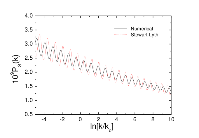
Figure 1: Plot of the power spectrum with numerical results and Stewart-Lyth approximation. In the calculation, we take $f=0.95M_{pl}$, $\delta N^{2}\approx 11$ ($\delta=-3\times 10^{-5},N=599$). $k_{c}$ is taken to be $k_{c}=7.0a_{0}H_{0}$.

Our results show that for $\delta N^{2}<1$, the Stewart-Lyth formula works well and the relative error is within $1\%$ in comparison with the numerical results. However, for $\delta N^{2}>1$, which we will discuss in detail in section V, the error could be large. In Fig.1, we plot $P_{S}(k)$ with numerical results and the Stewart-Lyth approximation. One can see that the difference is about 30 percent; for gravitational waves, the difference is little.

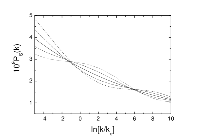
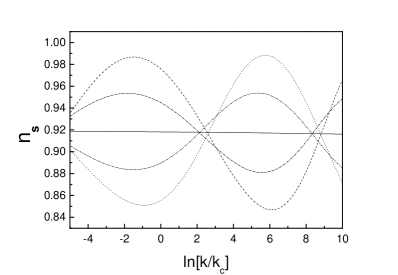
Figure 2: Modulation of the power spectrum and index, with $f=0.7M_{Pl}$, $\Lambda^{4}=2.0\times 10^{-13}M_{Pl}^{4}$. From left top to bottom, the lines stand for $\delta N^{2}=0.8,0.42,0,-0.42,-0.8$ respectively.

In the natural inflation model, the scalar spectrum index $n_{s}$ is generally smaller than 1. The $\delta$ term in our inflaton potential induces a modulation on the power spectrum. In Fig. 2, we plot the primordial scalar spectrum and index for a typical set of model parameters: $f=0.7M_{Pl}$, and $\Lambda^{4}=2.0\times 10^{-13}M_{Pl}^{4}$. As can be seen from the figures, the amplitude of the modulation in this model could be $\mathcal{O}(10\%)$.

Before concluding this section we should point out that the size of the modulation depends on the parameters of the model, and $P_{S}(k)$ behaves quite differently for small and large $f$. This can be understood qualitatively from the following two equations for natural inflation in the SR regime (Here we’ve set $8\pi G=1$) :

$$\frac{d\phi}{d\ln a}\sim\frac{\frac{1}{f}\sin(\phi/f)}{1+\cos(\phi/f)},$$ (38)

and

$$\phi_{\mathcal{N}}=2f\arcsin(\frac{\sqrt{2}f}{\sqrt{1+2f^{2}}}e^{-\frac{\mathcal{N}}{2f^{2}}}),$$ (39)

where $\mathcal{N}$ is the number of $e$-$folding$ between the corresponding horizon exit and the end of inflation . For smaller $f$, $\phi_{\mathcal{N}}$ would be much smaller than for larger $f$. For example $\phi_{\mathcal{N}}\approx 2.03$ for $f=0.95M_{Pl}$, while $f=0.4M_{Pl}$ gives $\phi_{\mathcal{N}}\approx 6.3\times 10^{-4}$ for a given number of $e$-$folding$ $\mathcal{N}=70$. Such a small $\phi$ for $f=0.4M_{Pl}$ would also make $\frac{d\phi}{d\ln a}$ much smaller than $f=0.95M_{Pl}$. This is also true for our model when SRA is well satisfied.

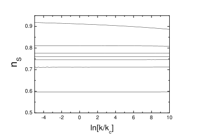
Figure 3: The same as Fig.2, however with different model parameters, $f=0.4M_{Pl}$, $\Lambda^{4}=5.0\times 10^{-17}M_{Pl}^{4}$. From above, the lines represent $\delta N^{2}$=$-0.7$, $-0.2$, $-0.07$, $0$, $0.07$, $0.2$, $0.7$ respectively.

In Fig.3, we plot the $P_{S}(k)$ and $n_{S}(k)$ for a small $f$. One can see from this figure that for $f=0.4M_{Pl}$, $P_{S}(k)$ has lost the feature of oscillation in the range of scale relevant to CMB and LSS, but the amplitudes of $P_{S}$ and $n_{S}$ change a lot.

IV Results and comparison with observations

In this section we study the implications of our model on CMB and LSS. The matter power spectrum is related to the primordial scalar power spectrum by

$$P(k)=T^{2}(k)P_{S}(k),$$ (40)

where $T(k)$ is the matter transfer function, which can be calculated for a given set of the cosmological background parameters. The matter power spectrum in a large range of scales can now be obtained by combining different data sets of CMB and LSS measurementsTZ02 . For example, currently the Lyman alpha forest probes comoving scale of $0.1\sim 10hMpc^{-1}$, the 2dF galaxy correlation $0.01\sim 0.1hMpc^{-1}$, and CMB measurements $0.001\sim 0.1hMpc^{-1}$. The CMB anisotropy is related to the primordial scalar power spectrum byMB95

$$\langle\Delta(\vec{n}_{1})\Delta(\vec{n}_{2})\rangle\equiv\frac{1}{4\pi}\sum\limits_{l=0}^{\infty}(2l+1)C_{l}P_{l}[\cos(\vec{n}_{1}\cdot\vec{n}_{2})],$$ (41)

$$C_{l}\equiv\frac{2\pi}{l(l+1)}\tilde{C_{l}}=\frac{4\pi}{(2l+1)}\int\frac{dk}{k}T_{l}^{2}(k)P_{S}(k),$$ (42)

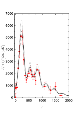
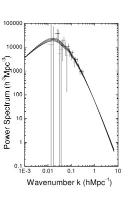
Figure 4: The CMB anisotropy and matter power spectrum for the parameters shown in Fig. 2, with $\delta N^{2}=0.8,0.42,0,-0.42,-0.8$ from above. The observational LSS data is from the PSCZ catalogueHT .

where $T_{l}(k)$ is the photon transfer function, which can be calculated for a given set of the cosmological parameters. Here $C_{l}$, $\tilde{C_{l}}$ and $T_{l}$ stand for the temperature angular power spectrum and transfer function. We’ve omitted the subscript $T$ for simplicity. We calculate $C_{l}$ by modifying the publicly available CMBFAST Seljak ; CMBFAST code. Similar calculations for running $n_{S}$ have been performed in, for example, Refs. Chung00 ; MT01 ; Covi . The fiducial model adopted in our calculation is the best fit model of Ref. Wang01 : $h=0.64,\Omega_{\Lambda}=0.66,\Omega_{b}h^{2}=0.02$ and $\Omega_{k}=0$. We used the combined CMB data set from Ref.MM02 in our plots. In Fig. 4 we plot the CMB angular power spectrum and the matter power spectrum with the primordial power spectrum shown in Fig.2. One can see that the theoretical predictions of our model are quite different from that with $\delta=0$ and the CMB data disfavor the case with $\delta N^{2}=0.8$.

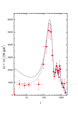
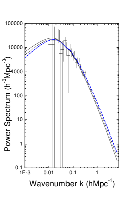
Figure 5: $\tilde{C_{l}}$ (left) and matter power spectrum (right) for a fixed $f=0.4M_{Pl}$ but different values of other model parameters. For the solid line, $\Lambda^{4}=1.3\times 10^{-16}M_{Pl}^{4}$, $\delta N^{2}=0$; The dotted line stands for $\Lambda^{4}=3.6\times 10^{-16}M_{Pl}^{4}$, $\delta N^{2}=-0.34$; For the dashed line, $\Lambda^{4}=5.2\times 10^{-16}M_{Pl}^{4}$, $\delta N^{2}=-0.78$.

One interesting point of our model is the running behavior of $n_{s}$ in the case with a small $f$, which we have shown in Fig. 3. One can see that without $\delta$ term the model predicts $n_{s}$ below 0.8, which is ruled out already by the data. However with the help of the $\delta$ term the theoretical predictions can be made to be consistent with the observations which can be seen from Fig. 5. Numerically in natural inflation with $f=0.4M_{pl}$ it predicts $n_{S}\approx 0.76$. And the fine tuning of the $V_{0}$ would not be able to make the theory consistent with $C_{l}$ and $P(k)$ Wang01 . However the presence of the $\delta$ term makes the fit better.

Up to now we have restricted ourself to the parameter space $\delta N^{2}<1$, however it would be interesting to take the potential in Eq. (7) as a phenomenological model and study the cosmological implications with an extended parameter space $\delta N^{2}>1$ . In this case, there are four parameters, where we take $f$ , $N$ and $\delta$ free, however $\Lambda$ can be normalized by observations.

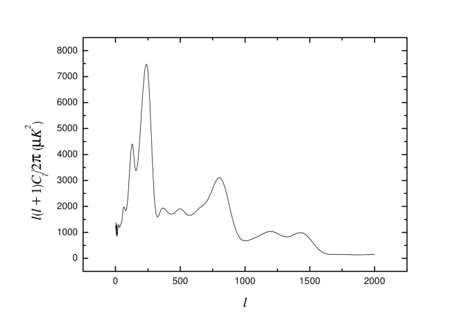
Figure 9: Theoretical prediction on $C_{l}$ with $f=.95M_{pl}$, $\delta=0.0007$ and $N=799$.

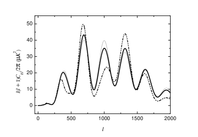
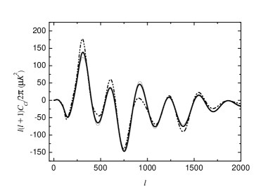
Figure 10: CMB polarization for the same parameters as in the right panel of Fig. 8 .

The effect of the modulation on the power spectrum depends on the amplitude, frequency, and phase. And the effect is more apparent for a high frequency (large $N$), as can be seen in Figs. 6-10. In Fig. 6 we take $N=599$ and find the variation of primordial scalar spectrum index is very frequent and its amplitude changes from about $0.3$ to $1.6$, although the value of $\delta$ is very small. However, our results also show that the tensor perturbation $P_{T}$ changes little since $\epsilon\ll 1$. We have checked the validity of the consistency relationCR0 . One can see from Fig. 7 for different range of $k$, $|n_{T}|$ is larger or smaller than $P_{T}/P_{S}$. The reason responsible for the violation of consistency relation in our model is due to a large running of $\beta$ from $-0.3$ to $0.3$ , which indicates SRA isn’t satisfied well. However, we will show below that this type of primordial spectrum doesn’t contradict to the current observations. In Fig.8 we plot the CMB anisotropy and the matter power spectrum for the given parameters and find that there can be a clear modulation on the matter power spectrum, which is somewhat similar to the baryonic oscillation wiggles, but has an entirely different origin. Of course, at present there is no observational evidence of such wiggles in the power spectrum. The peaks found in recent CMB measurements seem to agree reasonably well with the predictions of power law primordial spectrum. In the large scale structure data, there is some tentative report on wiggles in the power spectrum P01 ; M01a ; M01b ; H02 . These are generally thought to be due to baryonic oscillation, but the effect discussed here could also give rise to such wiggles. Since the position and frequency of the baryonic wiggles can be predicted, and there is no reason to expect that the primordial power spectrum modulation to coincide with it, there is hope to distinguish these two cases with high precision data. However, we note that at present time there is still no clear evidence even for the baryonic wiggles Xu ; MNC02 . Note that the modulation on the power spectrum is coherent, with different $P_{S}$ the shape of the CMB peaks can be also quite different, some would drastically change the structure of the $\tilde{C_{l}}$ spectrum, the peaks of the $\tilde{C_{l}}$ can be split into two in some particular cases. In the left panel of Fig.8, the first peaks have been clearly split, while in Fig.9, it shows that the original first and second peaks have been split, the third peak is highly raised and new peaks are also generated. In Fig. 10 we plot the CMB polarizations which are given by

$$C_{El}=\frac{4\pi}{(2l+1)}\int\frac{dk}{k}T_{El}^{2}(k)P_{S}(k),$$ (43)

$$C_{Cl}=\frac{4\pi}{(2l+1)}\int\frac{dk}{k}T_{l}(k)T_{El}(k)P_{S}(k)$$ (44)

for the E-mode and cross correlation spectrum polarization. These effects might be detectable by further CMB observationsPlank .

Current CMB observations do not exclude entirely the oscillating primordial spectrums. Consider the difference between $\tilde{C_{l}^{0}}$ and $\tilde{C}_{l}^{1}$ where $\tilde{C_{l}^{0}}$ is calculated with $f=0.95M_{pl}$, $\delta=0$ ($n_{S}\approx 0.945$) and $\tilde{C}_{l}^{1}$ with $f=0.95M_{pl}$ , $N=599$ , $\delta=-3\times 10^{-5}$, then compare them with the cosmic variancevariance limits on $\tilde{C_{l}^{0}}$. In Fig.11, the solid line stands for $\frac{\tilde{C}_{l}^{1}-\tilde{C}_{l}^{0}}{\tilde{C}_{l}^{0}}$ and the region between the dashed lines is given by the cosmic variance limits. Here $\tilde{C}_{l}^{1}$ and $\tilde{C}_{l}^{0}$ are normalized by COBE. Cosmic variance plays a fundamental limit to the $\tilde{C_{l}}$ spectrum that can be measured, with

$$\frac{\Delta\tilde{C_{l}}}{\tilde{C_{l}}}\geq\sqrt{\frac{2}{2l+1}}.$$ (45)

One can see from Fig.11 that $\tilde{C}_{l}^{1}$ and $\tilde{C}_{l}^{0}$ are hardly distinguishable. Even though the primordial spectrum (see, Fig.6) is oscillating, its contribution to CMB, because of being averaged over multiple l, becomes insignificant in this case.

V Discussions and Summary

In this paper we present a model which is a variation of natural inflation. We have shown two features of the primordial spectrum of this model, oscillating and scale-dependence and studied the implications on CMB and LSS. In the presence of the $\delta$ term the parameter space allowed for a successful natural inflation will be enlarged relative to the original natural inflation modelMT01 . When the parameter space is enlarged and extended to $\delta N^{2}>1$ for example due to some other physical motivationsFLZZ , there are several additional interesting effects. Although the SR approximation is violated and the spectral index oscillates with a large scale variation, there could be a large parameter space not ruled out by the observations. As we can see from Fig.8 when we gradually increase the value of $\delta$ the effects on CMB firstly take place on the first peak which can be slightly split, meanwhile wiggles on the matter power spectrum are gradually enhanced. The effects on CMB first peak and large scale structure are potentially observable and can be tested by future precise experiments.

In summary we have studied in this paper a model which is a variation of natural inflation and show that there are some interesting phenomenological features of this model, such as oscillating and scale-dependence in the primordial spectrums. And we have also discussed their implications on CMB and LSS.

Acknowledgments We thank R. Brandenberger for comments and suggestions on the manuscript. This work is supported in part by National Natural Science Foundation of China under Grant No.90303004 and by Ministry of Science and Technology of China under Grant No.NKBRSF G19990754.

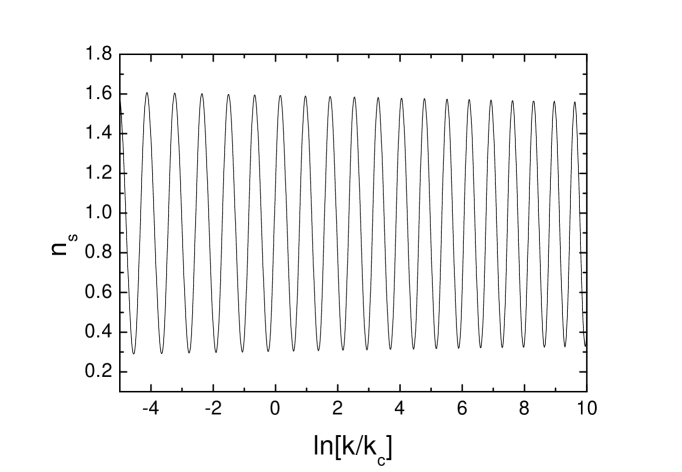
Figure 6: The primordial power spectrum index for $f=0.95M_{Pl}$, $N=599$, $\delta=-3\times 10^{-5}$.

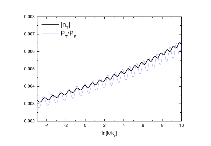
Figure 7: Plot of $|n_{T}|$ and $P_{T}/P_{S}$ for $f=0.95M_{Pl}$, $N=599$ and $\delta=-3\times 10^{-5}$.

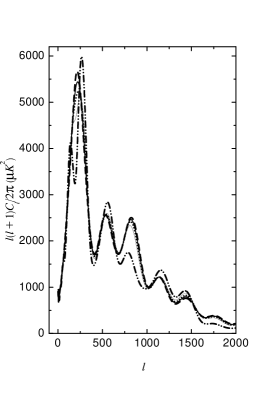
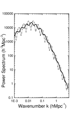
Figure 8: CMB anisotropy and matter power spectrum for $f=0.95M_{Pl},N=599$. Left panel: the dash dot dotted, the dashed, the dotted, the thicker solid and the thinner solid line stand for $\delta=-3\times 10^{-4}$, $\delta=3\times 10^{-5}$, $\delta=-3\times 10^{-5}$, $\delta=0$ and $\delta=-8\times 10^{-5}$ respectively; Right panel: The dash dotted dot, the thicker solid and the thinner solid stand for $\delta=-3\times 10^{-4}$, $\delta=-8\times 10^{-5}$ and $\delta=-3\times 10^{-5}$ respectively.

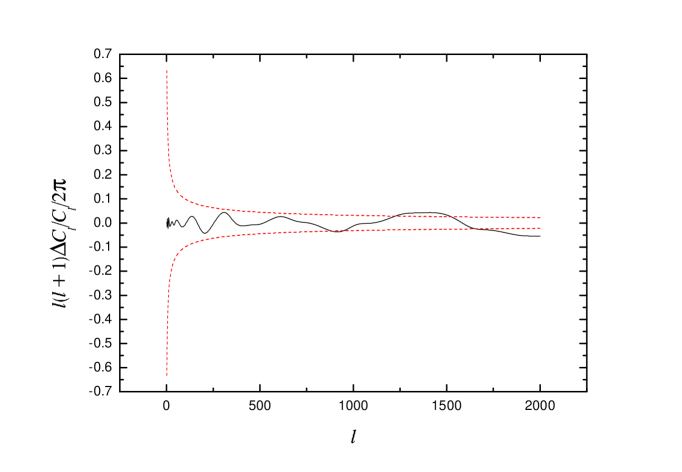
Figure 11: Plot of $\Delta\tilde{C_{l}}$ and the cosmic variance limits.

References

- (1) P. de Bernardis et al., Nature 404, 955 (2000).
- (2) A. E. Lange et al., Phys. Rev. D 63, 042001 (2001).
- (3) S. Hanany et al., Astrophys. J. Lett. 545, L5 (2000).
- (4) A. Balbi et al, Astrophys. J. Lett. 545, L1 (2000).
- (5) A. H. Jaffe et al., Phys. Rev. Lett. 86, 3475 (2001).
- (6) D. H. Lyth and A. Riotto, Phys.Rept. 314, 1 (1999).
- (7) X. Wang, M. Tegmark, M. Zaldarriaga, Phys. Rev. D 65, 123001 (2002).
- (8) J. E. Lidsey, A. R. Liddle, E. W. Kolb, E. J. Copeland and T. Barreiro, Rev. Mod. Phys. 69, 373 (1997).
- (9) S. Hannestad, Phys. Rev. D 63, 043009 (2001)
- (10) M. Matsumiya, M. Sasaki, J. Yokoyama, Phys. Rev. D 65, 083007 (2001).
- (11) Y. Wang, G. J. Mathews, Astrophys. J. 573, 1 (2002).
- (12) L. A. Kofman, A. D. Linde, A. A. Starobinsky, Phys. Lett. B 157, 361 (1985).
- (13) A. A. Starobinsky, JETP. Lett. 55, 489 (1992).
- (14) J. A. Adams, G. G. Ross, S. Sukar, Nucl. Phys. B 503, 405 (1997).
- (15) J. Lesgourgues, D. Polarski, A. A. Starobinsky, Mon. Not. R. Astron. Soc. 297, 769 (1998).
- (16) D. J. J. Chung, E. W. Kolb, A. Riotto and I. I. Tkachev, Phys. Rev. D 62, 043508 (2000).
- (17) L. Wang, M. Kamionkowski, Phys. Rev. D 61, 3504 (2000).
- (18) J. Lesgourgues, Nucl. Phys. B 582, 593 (2000).
- (19) L. M. Griffiths, J. Silk, S. Zaroubi, astro-ph/0010571.
- (20) S. Hannestad, S. H. Hansen, F. L. Villante, Astropart. Phys. 16, 137 (2001).
- (21) J. Barriga, E. Gaztanaga, M. Santos and S. Sarkar, Mon. Not. R. Astron. Soc. 324, 977 (2001).
- (22) M. Gramann, G. H’́utsi, Mon. Not. R. Astron. Soc. 327, 538 (2001).
- (23) M. Kamionkowski, A. R. Liddle, Phys. Rev. Lett. 84, 4525 (2000); A. R. Zentner, J.S. Bullock astro-ph/0205216.
- (24) D.N.Spergel, P.J.Steinhardt, Phys. Rev. Lett. 84, 3760 (2000).
- (25) B.D.Wandelt, et al. Proceedings of Dark Matter 2000 in press,astro-ph/0006344.
- (26) M. Kaplinghat, L. Knox and M. S. Turner, Phys. Rev. Lett. 85, 3335 (2000).
- (27) W.Lin, D.H. Huang , X. Zhang and R. Brandenberger Phys. Rev. Lett. 86, 954 (2001).
- (28) P.Bode, J.P.Ostriker, N.Turok , Astron. J. 556, 93 (2001).
- (29) A. Tasitsiomi,astro-ph/0205464.
- (30) K. Freese, J. A. Frieman, and A. V. Olinto, Phys. Rev. Lett. 65, 3234 (1990).
- (31) F. C. Adams, J. R. Bond, K. Freese and J. A. Frieman, A. V. Olinto, Phys. Rev. D 47, 426 (1993).
- (32) T. Moroi, T. Takahashi, Phys. Lett. B 503, 376 (2001).
- (33) J. Martin and R.H. Brandenberger, Phys. Rev. D 63, 123501 (2001); R.H. Brandenberger and J. Martin, Mod. Phys. Lett. A 16, 999 (2001); J.C. Niemeyer, Phys. Rev. D 63, 123502 (2001); J.C. Niemeyer and R. Parentani, , 101301(R) (2001); A. Kempf, , 083514 (2001); A. Kempf and J.C. Niemeyer, , 103501 (2001); R.Easther, B.R. Greene, W.H. Kinney and G.Shiu, hep-th/0110226; R.H. Brandenberger and J. Martin hep-th/0202142.
- (34) N. Kaloper, M. Kleban, A. Lawrence, and S. Shenker, hep-th/0201158.
- (35) G. Shiu and I. Wasserman, Phys. Lett. B 536, 1 (2002).
- (36) M. Kamionkowski and J. March-Russell, Phys. Lett. B 282, 137 (1992); R. Holman, , Phys. Lett. B 282, 132 (1992); S.M. Barr and D. Seckel, Phys. Rev. D 46, 539 (1992).
- (37) V. F. Mukhanov, H. A. Feldman, and R. H. Brandenberger, Phys.Rept. 215, 203 (1992).
- (38) E.D. Stewart and D.H. Lyth, Phys. Lett. B 302, 171 (1993).
- (39) D. H. Huang, W. B. Lin and X. M. Zhang, Phys. Rev. D 62, 087302 (2000).
- (40) J. Adams, B. Cresswell and R. Easther, Phys. Rev. D 64, 123514 (2001).
- (41) see e.g., M. Tegmark, M. Zaldarriaga, astro-ph/0207047.
- (42) see e.g. C. P. Ma and E. Bertschinger, Astrophys. J. 455, 7 (2995).
- (43) U. Seljak, M. Zaldarriaga Astrophys. J. 469, 437 (1996).
- (44) http://physics.nyu.edu/matiasz/CMBFAST/cmbfast.html.
- (45) D. H. Lyth and L. Covi, Phys. Rev. D 62, 103504 (2000).
- (46) M.Tegmark and M.Zaldarriaga,astro-ph/0207047.
- (47) A. J. S. Hamilton, M. Tegmark Mon. Not. R. Astron. Soc. 330, 506 (2002).
- (48) A.A. Starobinsky, Sov. Astron. Lett 11, 133 (1985); Stewart and D.H. Lyth, Phys. Lett. B 302, 171 (1993).
- (49) L. Hui and W. Kinney, Phys. Rev. D 65, 103507 (2002).
- (50) W. J. Percival et al., Mon. Not. R. Astron. Soc. 327, 1297 (2001).
- (51) C. J. Miller, R. C. Nichol, and D. J. Batuski, Science 292, 2302 (2001).
- (52) C. J. Miller, R. C. Nichol, and D. J. Batuski, Astrophys. J. 555, 68 (2001).
- (53) F. Hoyle et al., Mon. Not. R. Astron. Soc. 329, 336 (2002).
- (54) M. Tegmark, A. J. S. Hamilton, and Y.Xu, astro-ph/0111575.
- (55) C. J. Miller, R. C. Nichol, X. Chen, astro-ph/0207180.
- (56) http://astro.estec.esa.nl/Planck/.
- (57) , M. Zaldarriaga and U. Seljak, Phys. Rev. D 55, 1830 (1997); M. Kamionkowski, A. Kosowsky, and A. Stebbins, Phys. Rev. D 55, 7368 (1997).
- (58) B. Feng, M. Li, R.-J. Zhang, and X. Zhang, Phys. Rev. D 68, 103511 (2003).