Clustering statistics in cosmology

Abstract

The main tools in cosmology for comparing theoretical models with the observations of the galaxy distribution are statistical. We will review the applications of spatial statistics to the description of the large-scale structure of the universe. Special topics discussed in this talk will be: description of the galaxy samples, selection effects and biases, correlation functions, Fourier analysis, nearest neighbor statistics, Minkowski functionals and structure statistics. Special attention will be devoted to scaling laws and the use of the lacunarity measures in the description of the cosmic texture.

1 INTRODUCTION

Cosmology is a science which is experiencing a great development in the last decades. The achievements in the observations are driven the subject into an era of precision. The two fundamental pillars upon which observational cosmology rests are the cosmic microwave background and the distribution of the galaxies. The analysis of the huge amount of data that is now being collected in both areas will provided a unified framework to explain the formation and evolution of the large-scale structure in the universe. In this paper we will review some of the aspects related with the galaxy clustering.

2 OBSERVATIONS OF THE GALAXY CLUSTERING

2.1 Distances

Astronomers can accurately measure the galaxy positions on the sky. Unfortunately, it is not possible to have the same accuracy for the radial distance of each object. Different distance estimators are used in astronomy (see, for example, Ref. 1 for a review). For the luminosity selection effects one has to use the luminosity distance $D_{l}$, for the angular selection effects the angular diameter distance $D_{a}$, and in order to describe spatial clustering the comoving distance $r$ is used. All these distances can be derived from the cosmological redshift of the galaxy $z_{\mbox{\scriptsize cos}}$. Distances however depend on the adopted cosmological model and the value of its parameters. For nearby galaxies, the Hubble law states that $cz_{\mbox{\scriptsize cos}}=H_{0}r$ where $H_{0}$ is the present value of the Hubble parameter. Recent measurementsFreedman01 provide a value of $H_{0}=72\pm 8$ km s^-1 Mpc^-1. As space is curved, for more distant galaxies the distance-redshift relation is not linear any more, and different distances differ. We illustrate this in Fig. 1, where the different cosmological distances are given for the presently popular ’concordance model’. The statistics describing spatial clustering obviously depend on the adopted distance definitions, and thus on the prior cosmological model. This should be kept in mind, as these statistics are frequently used to estimate the ’true’ parameters of the cosmological model.

Figure 1: Different distance measures for a currently popular ’concordance’ model universe. Here $D_{l}$ is the luminosity distance, $r$ is the comoving distance, $D_{m}$ is the usually used Mattig distance (not defined for this model), and $D_{a}$ is the angular diameter distance. All distances are given in the units of the Hubble length $c/H_{0}$.

It is important to mention that the true cosmological redshift is not a measurable quantity since what we really are able to measure for each galaxy is a quantity $z$ satisfying the relation $cz=cz_{\mbox{\scriptsize cos}}+v{\mbox{\scriptsize pec}}$ where $v{\mbox{\scriptsize pec}}$ is the line-of-sight peculiar velocity. Peculiar velocities create a distorted version of the galaxy distribution —namely the redshift space—, as opposed to the real space where galaxies lie at their real positions. Distortions are more severe within the high density regions where effects like the Fingers-of-God —elongated structures along the line-of-sight— are the most evident consequenceveldist . In next sections we will discuss how this distortions affect the statistical clustering measures.

2.2 Recent redshift surveys

Cosmology, like many other modern scientific branches, is technology driven. Nowadays, use of multi-fiber spectrographs permits to measure the redshifts of many galaxies in a single run. Numbers have changed from 5-10 redshifts of galaxies measured per night in the 70s to 2000 redshifts per night at the late 90s. The reachable magnitude limit has moved from 14 to 19.5 in the blueguzzo02 . On the basis of this technology, new huge surveys of redshifts of galaxies are being built. The main two ongoing projects are the 2dF (2-degree Field) and the SDSS (Sloan Digital Sky Survey). More information about these surveys can be found in their Web pages: http://www.mso.anu.edu.au/2dFGRS/  for the 2dF survey and http://www.sdss.org/  for the SDSS survey.

In Fig. 2 we show cone diagrams of these two samples under construction. The visual analysis of these plots reveals the characteristic patterns already noticed in the famous first slice of the universelapparent (also shown in the diagram): a bubbly structure in which filaments and walls surround empty regions nearly devoid of galaxies. The big clusters of galaxies lie typically in the intersections of this labyrinth of structures.

Nevertheless, the new surveys display an important difference with respect to the older shallower slices: The depth of the surveys —being now several times larger— has allowed, for the first time, to be sure that the observed structures are much smaller than the size of the survey itself. This was not the case at the end of the 80s when the first Center for Astrophysics (CfA) slice was compiled. At that time it was not clear if the observed large-scale structures were going to increase in size with the survey depth. The first serious evidence on the contrary came with the Las Campanas Redshift Survey (LCRS)lcrs ; mart99 . This survey represented the beginning of the endkir96 in the sense that the characteristic structures of the galaxy distribution —voids, walls, and filaments— reached a maximum size and no structures of larger size were observed, as it should be expected if the distribution of galaxies was to be an unbounded fractalmart02 . This trend has been reinforced by the 2dF and Sloan first cone diagrams (see Fig. 2).

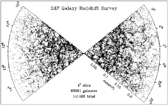
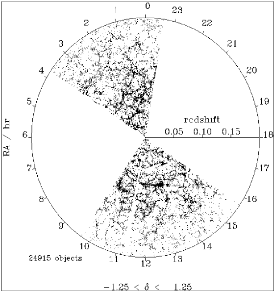
Figure 2: The top panel shows two $4^{\circ}$ slices with 63,381 galaxies from the 2dF redshift survey. The maximum depth is $z=0.25$, (figure from Peacock et al.2dfnature ). The bottom panel shows two $2.5^{\circ}$ slices with 24,915 galaxies from the SDSS survey. The outer circle has redshift $z=0.2$ (figure from Lovedayloveday ). As an inset, the first CfA slice from de Lapparent, Geller, and Huchralapparent is shown to scale.

2.3 Selection effects

One characteristic feature of these plots is that at larger distances the number of galaxies decreases. This phenomenon is entirely due to the way the surveys are built: they are flux-limited, therefore only the galaxies bright enough to have an apparent magnitude exceeding the survey cutoff are detected. At larger distances it is only possible to observe the intrinsically most luminous galaxies. To account for this incompleteness in the statistical analysis of these surveys, one needs to know the selection function $\varphi(r)$, which basically provides the probability that a galaxy at a given distance $r$ is included in the sample. This is the radial selection function that is usually estimated from the —previously calculated— luminosity function, $\phi(L)$. The luminosity function is defined by the number density of galaxies in a given range of intrinsic luminosity $[L,L+dL]$, $\phi(L)dL$. This function varies with morphological type, environmental properties and redshift due to galactic evolution. Traditionally it has been empirically fitted to a Schechter functionSchechter76

$$\phi(L)dL=\phi_{\ast}\left({L\over L_{\ast}}\right)^{\alpha}\exp\left(-{L\over L_{\ast}}\right)d\left({L\over L_{\ast}}\right),$$ (1)

where $L_{\ast}$ is a characteristic luminosity which separates the faint galaxy range where the power-law with exponent $\alpha$ dominates Eq. 1 and the bright end where the number density decreases exponentially.

Other selection effects affect the galaxy samples. Many of them are directional. Some are due to the construction of the sample: masks in given fields, fiber collisions in the spectrographs, etc. In addition, the sky is not equally transparent to the extragalactic light in all directions due to absorption of light performed by the dust of the Milky Way. Since the shape of our own Galaxy is rather flat, the more obscured regions are those with low values of $|b|$ (where $b$ is the galactic latitude). This effect has to be considered when computing the real brightness of a galaxy, which therefore depends on the direction of the line-of-sight. The best way to take this effect into account is to consider the well defined maps of the distribution of galactic dustdust .

For very deep samples, the absolute magnitude has to be estimated considering other adjustments like the K-correction, which takes into account that the luminosity of the galaxies at large redshift is detected at longer wavelength than actually was emitted.

Once the selection effects have been considered, the statistical analysis of the galaxy surveys are performed assigning to each galaxy a weight inversely proportional to the probability that the galaxy was included in the sample. A more clean solution is to consider volume-limited samples at the price of throwing away a huge amount of the collected data: At a given distance limit, one can easily calculate the absolute magnitude of a galaxy having the apparent magnitude limit of the survey. All galaxies intrinsically fainter that this absolute magnitude cutoff will be ignored in the volume-limited sample. An illustration of this procedure is shown in Fig. 3.

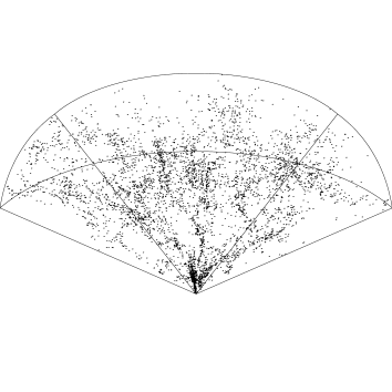
Figure 3: The left panel shows a region in the northern hemisphere of the CfA apparent magnitude limited sample. The apparent magnitude cutoff is $m=15.5$. It contains nearly 5000 galaxies. The right panel shows the same region when considered volume-limited sample. Now only the 905 galaxies brighter than $-19.70+5\log h$ has been included. The drop of the galaxy density with the distance to the observer (located at the vertex) appreciated in the left panel is not longer observed in the volume-limited sample.

3 CORRELATIONS

3.1 The two-point correlation function

The structure of the universe qualitatively described in the previous section needs to be quantified by means of statistical measures having the capacity of distinguish between different point patterns.

The most popular measure used in this context has been the two-point correlation functionpeeb80 ; sgd $\xi(r)$. The first time this quantity was applied to a galaxy catalog was in 1969 by Totsuji and Kiharatotsuji . Since then, its use has been widely spread. The quantity $\xi(r)$ is defined in terms of the probability that a galaxy is observed within a volume $dV$ lying at a distance $r$ from an arbitrary chosen galaxy,

$$dP=n[1+\xi(r)]dV,$$ (2)

where $n$ is the average galaxy number density. For a completely random distribution $\xi(r)=0$. Positive values indicate clustering, negative values indicate anti-clustering or regularity. In this definition, isotropy and homogeneity of the point process is being assumed, otherwise the function $\xi(r)$ should depend on a vector quantity.

Several estimators have been used to obtain the two-point correlation function from a given data setpons ; kerm . At short distances their results are nearly indistinguishable; at large distances, however, the differences become important. The best performance is reached by the Hamiltonham93 and the Landy and Szalaylandy93 estimators.

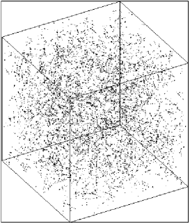
Figure 4: The top left panel shows a segment Cox process simulated on a cube with side-length 100. The top right panel shows the two-point correlation function: The dotted line corresponds to the expected analytical expression (see Eq. 3), that is, in this range of scales, close to a power-law with exponent $-2$. Solid bullets are the empirically calculated values of $\xi(r)$. Open diamonds correspond to the function calculated on the shifted point process with shifts following a power-law distribution function, while crosses correspond to Gaussian shifts. The left bottom panel shows a slice with dimensions $40\times 40\times 10$ drawn from the unshifted full realization. The same slice is shown after applying power-law shifts (central bottom panel) and Gaussian fits (right bottom panel).

To illustrate the kind of information that we can extract from this second-order spatial statistic we can use a point process having an analytic expression for its two-point correlation function. A segment Cox process is generated by randomly placing segments of length $\ell$ within a window $W$. Then, we scatter points on the segments with a given intensity. If the mean number of segments per unit volume is $\lambda_{s}$, the correlation function of the process has the formskm

$$\xi_{\rm{Cox}}(r)=\frac{1}{2\pi r^{2}\lambda_{s}\ell}-\frac{1}{2\pi r\ell^{2}\lambda_{s}},$$ (3)

for $r\leq\ell$ and vanishes for larger $r$. Note that this expression is independent of the number of points per unit length scattered on each segment.

In Fig. 4 we show a 3-D simulation of this process with parameters $\lambda_{s}=0.001$ and $\ell=10$. The correlation function estimate is shown together with the analytical expectation of Eq. 3. Note that, at small scales, $\xi_{\mbox{\scriptsize Cox}}(r)\sim r^{-\gamma}$ with $\gamma=2$. The strong clustering signal of this point field can be smeared out by applying independent random shifts to each point of the simulation. If the random shifts are performed by a three-dimensional Gaussian distributed vector with $\sigma=0.5$, the short scale correlations are completely destroyed (see Fig. 4). If the shifts are distributed according to a power-law density probability function $d^{\ast}(r)\propto r^{\alpha}$, the value of $\gamma$ is reduced by $2(1+\alpha)$. In the example $\alpha=-0.75$ and therefore $\gamma$ changes from $2$ to $1.5$. This seems to be a rather general phenomenonsnethlage . The random shifts affect the correlation function mimicking the way peculiar velocities suppress the short range correlationsmart93 (for scales $r\leq 2h^{-1}$ Mpc, where $h$ is the Hubble parameter in units of 100 km s^-1 Mpc^-1).

3.2 $\xi(r)$ on recent samples

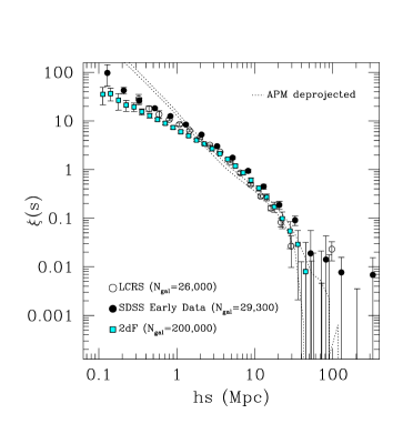
Figure 5: The two-point redshift correlation function for the deepest available redshift surveys: The Las Campanas Redshift SurveyTucker , the 2dF (Hawkins et al. —the 2dFGRS team—, in preparation), and the early public release of the Sloan Digital Sky SurveyZehavi . The dotted lines, that fit well a power law, correspond to the real-space correlation function deprojected from the APM angular data using two different models of galactic evolutionbaugh , (figure from Guzzoguzzo02 ).

Fig. 5 shows the two-point correlation function in redshift space calculated on three different deep redshift surveys: LCRSTucker , d2F (Hawkins et al. —the 2dFGRS team—, in preparation), and SDSSZehavi . The agreement is quite remarkable, in fact the differences between LCRS and SDSS are mainly due to the fact that comoving distances have been calculated assuming different cosmological models. It is clear that trying to fit reasonably well a power-law $\xi(s)=(s/s_{0})^{-\gamma}$ to the data is hopeless. In fact, the dotted lines show the real space correlation function calculated from the Automatic Plate Machine (APM) angular databaugh after deprojecting the angular correlation function with the Limber equation. Now, a reliable power-law $\xi(r)=(r/r_{0})^{-\gamma}$, with $\gamma=1.7$ and $r_{0}=4.1\,h^{-1}$ Mpc, can be fitted to the curves for scales $r\leq 4\,h^{-1}$ Mpc. The slope is in agreement with the results inferred by Zehavi et al.Zehavi for the SDSS early data: $\gamma=1.75\pm 0.03$ and $r_{0}=6.1\pm 0.2\,h^{-1}$ Mpc, within the range $0.1\leq r\leq 16\,h^{-1}$ Mpc. Although the APM amplitude was smaller, Baughbaugh reported an appreciable shoulder in $\xi(r)$ for scales $4\leq r\leq 25\,h^{-1}$ Mpc where the correlation function was rising above the fitted power law. The diagram also illustrates the effects of the peculiar velocities in redshift surveys suppressing the short-range correlations and enhancing the amplitude at intermediate scales due to coherent flows veldist ; guzzo02 . It is also interesting to note that the first zero crossing of the two-point correlation function occurs at scales around 30–40 $h^{-1}$ Mpc.

3.3 Fractal scaling

The number of neighbors —on average— a galaxy has within a sphere of radius $r$ is just the integral

$$N(<r)=n\int_{0}^{r}4\pi s^{2}(1+\xi(s))ds$$ (4)

When this function follows a power-law $N(<r)\propto r^{D_{2}}$, the exponent is the correlation dimension, and the point pattern is said to verify fractal scaling. There is no doubt that up to a given scale the galaxy distribution fits rather well the fractal picture. However, some controversy regarding the extent of the fractal regime has motivated an interesting debatepietronero ; davisprin ; guzzo ; mart99 . Nevertheless, the new data is showing overwhelming evidence that the correlation dimension is a scale dependent quantity. Different authors mart98 ; cappi98 ; wuetal ; scaramel ; hatton ; amend ; pancoles ; lcfrac ; colless have analyzed the more recent available redshift surveys using $N(r)$ or related measures with appropriate estimators. Their results show unambiguously an increasing trend of $D_{2}$ with the scale from values of $D_{2}\sim 2$ at intermediate scales to values of $D_{2}\sim 3$ at scales larger than 30 $h^{-1}$ Mpc. Moreover, one of the strong predictions of the fractal hypothesis is that the correlation length —the value $r_{0}$ at which the correlation function reaches the unity ($\xi(r_{0})=1$)— must increase linearly with the depth of the sample. This seems not to be the casedavis88 ; mart01 .

3.4 Lacunarity

If in a fractal distribution, we count for each point the total number of neighbors within a ball of radius $r$, $M(r)$, we can see that this quantity follows roughly a power-law

$$M(r)=Fr^{D},$$ (5)

the exponent $D$ is the so-called mass-radius dimension. Taking the average over all the points we get an estimate of the integral correlation function $N(<r)=\left\langle M(r)\right\rangle$. In this section, we show how the correlation dimension alone is not enough to characterize the fractal structure.

The variability of the prefactor $F$ in Eq. 5 can be used as a measure to distinguish between different fractal patterns having the same correlation dimension. This variability provides an indicator of the lacunarity. Several alternative quantitative measures have been proposed in the literatureAllain ; Plotnick ; Gaite . According to Ref. 43, we adopt the following numerical definition for the lacunarity, which is basically the second-order variability measure of the prefactor $F$ in Eq. 5,

$$\Phi=\frac{\left\langle(F-\left\langle F\right\rangle)^{2}\right\rangle}{\left\langle F\right\rangle^{2}}.$$ (6)

We first illustrate these measure on several two-dimensional point patterns.

1. Mandelbrotmand75 proposed an elegant fractal prescription to locate galaxies in space. It is the so-called Rayleigh-Lévy flight: galaxies are placed at the end points of a random walk with steps having isotropically random directions. The step length follows a power-law probability distribution function $P(r>\ell)=(\ell_{0}/\ell)^{D}$ for $\ell\geq\ell_{0}$ with $D<2$, and $P(r>\ell)=1$ for $\ell<\ell_{0}$. Panel (a) in Fig. 6 shows a two-dimensional simulation with $D=1.5$ and $\ell=0.001$ generated within a square with sidelength 1.

2. Soneira and Peeblessp proposed a hierarchical fractal model to mimic the statistical properties of the Lick galaxy catalog. This model is built as follows: Within a sphere of radius $R$ we place randomly $\eta$ spheres of radius $R/\lambda$ with $\lambda>1$. Now, in each of the new spheres, $\eta$ centers of smaller spheres with radius $R/\lambda^{2}$ are placed. This process is repeated until a given level $L$ is reached. Galaxies are situated at the centers of the $\eta^{L}$ spheres of the last level. The correlation dimension of this fractal clump is $\log(\eta)/\log(\lambda)$. Panel (b) in Fig. 6 shows a two-dimensional simulation with $\eta=2$, $\lambda=1.587$, and therefore $D_{2}=1.5$. Four clumps with $L=13$ have been generated within a disc of diameter 1.

3. The next example is a multiplicative cascade process performed on the unit squaremart90 . First, the square is divided into four equal pieces. We assign a probability measure to each of the pieces randomly permuted from the set $\{p_{1},p_{2},p_{3},p_{4}\}$. Each subsquare is divided again into four pieces, and again we attach a measure to each of the them by multiplying a $p_{i}$ value randomly permuted by the value corresponding to its parent square. The process is repeated several times, and in each step the measure attached to each small square is the product of a new $p_{i}$ value with all its ancestors. After $L$ steps, we end with a mass distribution over a $2^{L}\times 2^{L}$ lattice. A point process is then generated placing randomly points within each pixel with probability proportional to its measure. Panels (c) and (d) in Fig. 6 show two realizations of this model, one being a simple fractal, panel (c), with $p_{1}=p_{2}=p_{3}=1/3$, and $p_{4}=0$ and the other one being a multifractal measure, panel (d), with $p_{1}=0.4463,\,\;p_{2}=0.2537,\,\;p_{3}=0.3$, and $p_{4}=0$. While for the first case $D_{2}=\log 3/\log 2\simeq 1.58$, for the multifractal measure the chosen values of $p_{i}$ provide a dimensionality $D_{2}=1.5$.

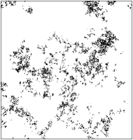
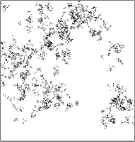
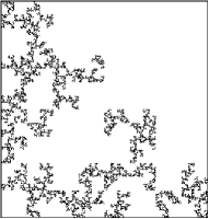
(a) (b) (c) (d)

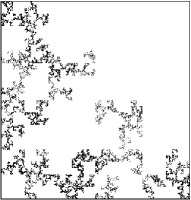
(e)

Figure 6: Panels (a)-(d) show different point patterns having similar correlation dimension: (a) Rayleigh-Lévy dust, (b) Soneira and Peebles model, (c) simple fractal distribution, (d) multifractal distribution. For all cases, the correlation integral follows a power law with similar exponent (panel (e) bottom). The central diagram in panel (e) shows the local correlation dimension calculated as the slope of the log-log linear regression within small portions of the scale range —the width of the sliding window is displayed by an arrow—. The lacunarity measure characterizing the textural properties of each point pattern is shown in the top diagram of panel (e).

The bottom panel of Fig. 6 shows the relation $\log N(<r)$ versus $\log r$ for the four examples. The power-law behavior $N(<r)\propto r^{D_{2}}$ is clearly appreciated in the diagram, with scaling exponent $D_{2}\simeq 1.6$ for all cases.

A more detailed analysis of the local correlation dimension is reported in the central diagram of panel (e), where we show how $D_{2}$ changes with the scale. In this case, $D_{2}$ has been calculated as the slope of the local linear regression fit to a small portion of the curve. This sliding window estimate of the local value of $D_{2}$ is very sensitive to any possible non fractal behavior that could not well be appreciated in the plot of $\log N(<r)$. The width of the sliding window used in the estimation is shown as an arrow in the bottom panel. We can see that in all the analyzed point patterns the empirical local correlation dimension oscillates around $D_{2}\simeq 1.6$. It is therefore rather hard to find significative differences between the analyzed patterns through the function $N(<r)$ or from $D_{2}(r)$.

The differences, however, are revealed by the lacunarity measure (Eq. 6) which is shown in the top diagram of panel (e). The lacunarity curves $\Phi(r)$, associated to each pattern, show clear differences between them providing us with a valuable information about the texture of each process.

The simple fractal model in panel (c) shows rather constant behavior of $\Phi$ with the scale, displaying only very small oscillations around $\Phi\simeq 0.1$. By contrast, the multifractal set, being quite similar to the eye to the simple fractal, shows a completely different lacunarity curve, with a characteristic monotonic decreasing behavior from $\Phi\simeq 0.7$, at the smallest scales, to $\Phi\simeq 0.2$ at the larger scales. In this case the lacunarity is associated to the inhomogeneous distribution of the measure on the fractal supportAllain ; Plotnick in which we can find highly populated regions (where the values of the measure are very large) together with other nearly empty locations (where the measure takes the lowest values). The lacunarity measure reveals the small scale heterogeneity of the multifractal set. Only at large scales the curve approaches that of the simple fractal pattern.

The lacunarity curve of the Soneira and Peebles model (panel (b)) is quite similar to that of the multifractal cascade model, with a decreasing behavior of $\Phi$ with the scale. We can see in the plot that $\Phi$ varies from $0.45$ at the smallest scales to $0.08$ at the largest analyzed distances. Because the different clumps overlap with each other, the set presents scale-dependent structure which cannot be discovered by analyzing the correlation function or the correlation dimension alone.

It is quite remarkable how the lacunarity curve of this model differs from the one corresponding to the Rayleigh–Lévy flight, although both spatial patterns seem quite similar to the eye. Within the first 2/3 of the analyzed scale range, the behavior of $\Phi$ with the scale, for the Rayleigh–Lévy dust, is rather flat with oscillations around $\Phi\simeq 0.4$. It is, therefore, qualitatively similar to the behavior of the simple fractal pattern, although showing a higher value of $\Phi$ and displaying oscillations with higher amplitude. The large-scale properties of finite regions of Rayleigh–Lévy dusts are extremely variable, and the rapid decrease of lacunarity at larger scales for the sample shown in panel (a) is typical only for dense subregions of a Rayleigh–Lévy flight.

4 POWER SPECTRUM

The power spectrum (power spectral density) is also a quadratic statistic of the spatial clustering, as is the two-point correlation function. Formally they are equivalent (the power spectrum is the Fourier transform of the correlation function), but they describe different sides of a process. The power spectrum is more intuitive physically, separating processes on different scales. Moreover, the model predictions are made in terms of power spectra. Statistically, the advantage is that the power spectrum amplitudes for different wavenumbers are statistically orthogonal:

$$E\left\{\widetilde{\delta}({\mathbf{k}})\widetilde{\delta}^{\star}({\mathbf{k}}^{\prime})\right\}=(2\pi)^{3}\delta_{D}({\mathbf{k}}-{\mathbf{k}}^{\prime})P({\mathbf{k}}).$$ (7)

Here $\widetilde{\delta}({\mathbf{k}})$ is the Fourier amplitude of the overdensity field $\delta=(\rho-\bar{\rho})/\bar{\rho}$ at a wavenumber ${\mathbf{k}}$, $\rho$ is the matter density, a star denotes complex conjugation, $E\{\}$ denotes expectation values over realizations of the random field, and $\delta_{D}({\mathbf{x}})$ is the three-dimensional Dirac delta function.

If we have a sample (catalog) of galaxies with the coordinates ${\mathbf{x}}_{j}$, we can write the estimator for a Fourier amplitude of the overdensity distributionfkp (for a finite set of frequencies ${\mathbf{k}}_{i}$) as

$$F({\mathbf{k}}_{i})=\sum_{j}\frac{\psi({\mathbf{x}}_{j})}{\bar{n}({{\mathbf{x}}}_{j})}e^{i{\mathbf{k}}_{i}\cdot{\mathbf{x}}}-\widetilde{\psi}({\mathbf{k}}_{i}),$$

where $\bar{n}({\mathbf{x}})$ is the position-dependent selection function (the observed mean number density) of the sample and $\psi({\mathbf{x}})$ is a weight function that can be selected at will.

The raw estimator for the spectrum is

$$P_{R}({\mathbf{k}}_{i})=F({\mathbf{k}}_{i})F^{\star}({\mathbf{k}}_{i}),$$

and its expectation value

$$E\left\{\langle|F({\mathbf{k}}_{i})|^{2}\rangle\right\}=\int G({\mathbf{k}}_{i}-{\mathbf{k}}^{\prime})P({\mathbf{k}}^{\prime})\,\frac{d^{3}k^{\prime}}{(2\pi)^{3}}+\int_{V}\frac{\psi^{2}({\mathbf{x}})}{\bar{n}({\mathbf{x}})}\,d^{3}x,$$

where $G({\mathbf{k}})=|\tilde{\psi}({\mathbf{k}})|^{2}$ is the window function that also depends on the geometry of the sample volume. Symbolically, we can get the estimate of the power spectra $\widehat{P}$ by inverting the integral equation

$$G\otimes\widehat{P}=P_{R}-N,$$

where $\otimes$ denotes convolution, $P_{R}$ is the raw estimate of power, and $N$ is the (constant) shot noise term.

In general, we have to deconvolve the noise-corrected raw power to get the estimate of the power spectrum. A sample of a characteristic spatial size $L$ creates a window function of width of $\Delta k\approx 1/L$, correlating estimates of spectra at that wavenumber interval.

As the cosmological spectra are usually assumed to be isotropic, the standard method to estimate the spectrum involves an additional step of averaging the estimates $\widehat{P}({\mathbf{k}})$ over a spherical shell $k\in[k_{i},k_{i+1}]$ of thickness $k_{i+1}-k_{i}>\Delta k=1/L$ in wavenumber space.

As the data set get large, straight application of direct methods (especially the error analysis) becomes difficult. There are different recipes that have been developed with the future data sets in mind. A good review of these methods is given in Ref. 48.

The deeper the galaxy sample, the larger the spectral resolution and the larger the wavenumber interval where the power spectrum can be estimated. Fig. 7 shows the power spectrum for the 2dF survey when contained 160,000 galaxies and had a depth of 750 $h^{-1}\,$Mpc. The power spectrum was calculated by the 2dF team (filled diamonds) using the direct method2dfpower . The covariance matrix of this power spectrum estimate was found from simulations of a matching Gaussian Cox process in the sample volume. The diagram shows also the results of the calculation performed by Tegmark et al.Tegmark01 over the first public release of the sample containing 102,000 redshifts (squares). Their paper is a good example of application of the large dataset machinery. They used compression of the raw data into (pseudo) Karhunen-Loéve eigenmodes and compressed these quadratically into band-powers, using the Fisher matrix formalism to obtain the final estimate of the power spectrumsgd ; future . For comparison, the power spectrum of the REFLEX cluster samplereflex (obtained by a direct method) is also shown. Clusters of galaxies form only at the highest peaks of the density field. This bias is the responsible for the larger amplitude of the power spectrum corresponding to the clusters of galaxies. The diagram also shows the curves for the power spectrum corresponding to different models of structure formation (see the caption for the details).

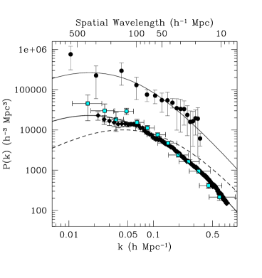
Figure 7: The power spectrum of the 2dF galaxy redshift survey calculated using two different estimators2dfpower ; Tegmark01 and for the X-ray built survey of clusters of galaxies REFLEX (filled circles)reflex . The dashed line correspond to an Einstein-de Sitter ($\Omega_{M}=1,\Omega_{\Lambda}=0$) CDM model that is clearly rejected by the observations. The $\Lambda$-CDM concordance model ($\Omega_{M}=0.3,\Omega_{\Lambda}=0.7,h=0.7$) is represented by solid lines with the appropriate bias parameters for both galaxies (bottom line) and clusters (top line), (figure from Guzzoguzzo02 .)

The main new feature in the spectra, obtained for the new deep samples, is the emergence of details (wiggles). Sometime ago, the goal was to estimate the overall behavior of the spectrum and, at most, to find its maximum, which is related with the homogeneity scale. The new data enables us to see and study the details of the spectrum. These wiggles could be interpreted as traces of acoustic oscillations in the post-recombination power spectrum. Similar oscillations are predicted for the cosmic microwave background radiation fluctuation spectrum. It seems, however, that the apparent wiggles detected in the 2dF power spectrum are an artifact due to the window function and other measurement technicalities2dfpower ; Tegmark01 ; guzzo02 .

5 OTHER CLUSTERING MEASURES

The correlation function can be generalized to higher ordersgd ; gazta ; peebval : The $N$-point correlation functions. This allows to statistically characterize the galaxy distribution with a hierarchy of quantities which progressively provide us with more and more information about the clustering of the point process. These measures, however, had been difficult to derive with reliability from the galaxy catalogs. The new generation of surveys will surely overcome this problem.

There are, nevertheless, other clustering measures which provide complementary information to the second-order quantities describe above. For example, the topology of the large-scale structure measured by the genus statisticgott provides information about the phase correlations of the density fluctuations in $k$-space. To obtain this quantity, first the point process has to be smoothed by means of a kernel function with a given bandwidth. The topological genus of a surface is the number of holes minus the number of isolated regions plus 1. This quantity is calculated for the isodensity surfaces of the smoothed data corresponding to a given density threshold. The genus has an analytically calculable expression for a Gaussian fieldadler .

Minkowski functionals are very effective clustering measures commonly used in stochastic geometryskm . These quantities are adequate to study the shape and connectivity of a union of convex bodies. They can easily be adapted to point processesmecke94 by considering the covering of the point field formed by sets $A_{r}=\cup_{i=1}^{N}B_{r}({\mathbf{x}}_{i})$ where $r$ is the diagnostic parameter, $\{{\mathbf{x}}_{i}\}_{i=1}^{N}$ represents the galaxy positions, and $B_{r}({\mathbf{x}}_{i})$ is a ball of radius $r$ centered at point ${\mathbf{x}}_{i}$. Minkowski functionalskercher97 are applied to sets $A_{r}$ as $r$ increases. In ${{{\rm I\kern-1.60004pt{}R}}}^{3}$ there are four functionals: the volume $V$, the surface area $A$, the integral mean curvature $H$, and the Euler-Poincaré characteristic $\chi$, related with the genus of the boundary of $A_{r}$.

Several quantities based on distances to nearest neighbors have been used in the cosmological literature. The empty space function $F(r)$ is the distribution function of the distance between a given random test particle in ${{{\rm I\kern-1.60004pt{}R}}}^{3}$ and its nearest galaxy. It is related with the void probability functionlachieze $P_{0}(r)$ —the probability that a ball of radius $r$ randomly placed contains no galaxies— by $F(r)=1-P_{0}(r)$. $G(r)$ is the distribution function of the distance $r$ of a given galaxy to its nearest neighbor. The quotient $J(r)=[1-G(r)]/[1-F(r)]$ has been successfully applied to describe the spatial pattern interaction in the galaxy distributionkerscher99 . Related with the nearest neighbor distances, the minimal spanning tree is a structure descriptor that has shown powerful capabilities to reveal the clustering properties of different point patternsmstbarrow ; mart90 ; doromst . The minimal spanning tree (MST) is the unique network connecting the $N$ points of the process with a route formed by $N-1$ edges, without closed loops and having minimal total length (the total length is the sum of the lengths of the edges). The frequency histograms of the MST edge lengths can be used to analyze the galaxy distribution and to compare it with the simulated modelsdoromst .

The use of wavelets and related integral transforms is an extremely promising tool in the clustering analysis of 3-D catalogs. Some of these techniques are introduced in other contributions published in this volumeuno ; dos .

- (1) V. J. Martínez and E. Saar, Statistics of the Galaxy Distribution, Chapman and Hall/CRC Press, Boca Raton, 2002.
- (2) W. L. Freedman, B. F. Madore, B. K. Gibson, L. Ferrarese, D. D. Kelson, S. Sakai, J. R. Mould, R. C. Kennicutt, H. C. Ford, J. A. Graham, J. P. Huchra, S. M. G. Hughes, G. D. Illingworth, L. M. Macri, and P. B. Stetson, “Final results from the Hubble Space Telescope Key Project to measure the Hubble constant,” Astrophys. J. 553, pp. 47–72, 2001.
- (3) A. J. S. Hamilton, “Linear redshift distortions: A review,” in The Evolving Universe, Astrophysics and Space Science Library 231, pp. 185–275, Kluwer Academic Publishers, (Dordrecht), 1998.
- (4) L. Guzzo, “Large-scale structure from galaxy and cluster surveys,” in DARK2002, 4th Heidelberg Int. Conference on Dark Matter in Astro- and Particle Physics, H.-V. Klapdor-Kleingrothaus and R. Viollier, eds., Springer–Verlag, 2002. In press, astro-ph/0207285.
- (5) V. de Lapparent, M. J. Geller, and J. P. Huchra, “A slice of the universe,” Astrophys. J. Lett. 302, pp. L1–L5, 1986.
- (6) S. A. Shectman, S. D. Landy, A. Oemler, D. L. Tucker, H. Lin, R. P. Kirshner, and P. L. Schechter, “The Las Campanas Redshift Survey,” Astrophys. J. 470, p. 172, 1996.
- (7) V. J. Martínez, “Is the universe fractal?,” Science 284, pp. 445–446, 1999.
- (8) R. P. Kirshner, “Galaxy redshift surveys,” in Dark Matter in the Universe, S. Bonometto, J. R. Primack, and A. Provenzale, eds., pp. 36–48, IOS Press, (Amsterdam), 1996.
- (9) V. J. Martínez, “Non-fractality on large scales,” in New Cosmological Data and the Values of the Fundamental Parameters, IAU Symposium, A. N. Lasenby and A. Wilkinson, eds., 201, Astronomical Society of the Pacific, San Francisco, 2002. In press.
- (10) J. A. Peacock, S. Cole, P. Norberg, C. M. Baugh, J. Bland-Hawthorn, T. Bridges, R. D. Cannon, M. Colless, C. Collins, W. Couch, G. Dalton, K. Deeley, R. D. Propris, S. P. Driver, G. Efstathiou, R. S. Ellis, C. S. Frenk, K. Glazebrook, C. Jackson, O. Lahav, I. Lewis, S. Lumsden, S. Maddox, W. J. Percival, B. A. Peterson, I. Price, W. Sutherland, and K. Taylor, “A measurement of the cosmological mass density from clustering in the 2dF galaxy redshift survey,” Nature 410, pp. 169–173, 2001.
- (11) J. Loveday, “The Sloan Digital Sky Survey,” Contemporary Physics , 2002. In press, astro-ph/0207189.
- (12) P. Schechter, “An analytic expression for the luminosity function for galaxies.,” Astrophys. J. 203, pp. 297–306, 1976.
- (13) D. J. Schlegel, D. P. Finkbeiner, and M. Davis, “Maps of dust infrared emission for use in estimation of reddening and cosmic microwave background radiation foregrounds,” Astrophys. J. 500, pp. 525–553, 1998.
- (14) P. J. E. Peebles, The Large-Scale Structure of the Universe, Princeton University Press, Princeton, 1980.
- (15) H. Totsuji and T. Kihara, “The correlation function for the distribution of galaxies,” Publ. Astron. Soc. Japan 21, p. 221, 1969.
- (16) M.-J. Pons-Bordería, V. J. Martínez, D. Stoyan, H. Stoyan, and E. Saar, “Comparing estimators of the galaxy correlation function,” Astrophys. J. 523, pp. 480–491, 1999.
- (17) M. Kerscher, I. Szapudi, and A. S. Szalay, “A comparison of estimators for the two-point correlation function,” Astrophys. J. 535, pp. L13–L16, 2000.
- (18) A. J. S. Hamilton, “Toward better ways to measure the galaxy correlation function,” Astrophys. J. 417, pp. 19–35, 1993.
- (19) S. D. Landy and A. S. Szalay, “Bias and variance of angular correlation functions,” Astrophys. J. 412, pp. 64–71, 1993.
- (20) D. Stoyan, W. Kendall, and J. Mecke, Stochastic Geometry and its Applications, John Wiley & Sons, Chichester, 1995.
- (21) M. Snethlage, V. J. Martínez, D. Stoyan, and E. Saar, “Point field models for the galaxy point pattern. Modelling the singularity of the two-point correlation function,” Astron. Astrophys. 388, pp. 758–765, 2002.
- (22) V. J. Martínez, M. Portilla, B. J. T. Jones, and S. Paredes, “The galaxy clustering correlation length,” Astron. Astrophys. 280, pp. 5–19, 1993.
- (23) D. L. Tucker, A. Oemler, R. P. Kirshner, H. Lin, S. A. Shectman, S. D. Landy, P. L. Schechter, V. Muller, S. Gottlober, and J. Einasto, “The Las Campanas Redshift Survey galaxy-galaxy autocorrelation function,” Mon. Not. R. Astr. Soc. 285, pp. L5–L9, 1997.
- (24) I. Zehavi, M. R. Blanton, J. A. Frieman, D. H. Weinberg, H. J. Mo, M. A. Strauss, S. F. Anderson, J. Annis, N. A. Bahcall, M. Bernardi, J. W. Briggs, J. Brinkmann, S. Burles, L. Carey, F. J. Castander, A. J. Connolly, I. Csabai, J. J. Dalcanton, S. Dodelson, M. Doi, D. Eisenstein, M. L. Evans, D. P. Finkbeiner, S. Friedman, M. Fukugita, J. E. Gunn, G. S. Hennessy, R. B. Hindsley, Ž. Ivezić, S. Kent, G. R. Knapp, R. Kron, P. Kunszt, D. Q. Lamb, R. F. Leger, D. C. Long, J. Loveday, R. H. Lupton, T. McKay, A. Meiksin, A. Merrelli, J. A. Munn, V. Narayanan, M. Newcomb, R. C. Nichol, R. Owen, J. Peoples, A. Pope, C. M. Rockosi, D. Schlegel, D. P. Schneider, R. Scoccimarro, R. K. Sheth, W. Siegmund, S. Smee, Y. Snir, A. Stebbins, C. Stoughton, M. SubbaRao, A. S. Szalay, I. Szapudi, M. Tegmark, D. L. Tucker, A. Uomoto, D. Vanden Berk, M. S. Vogeley, P. Waddell, B. Yanny, and D. G. York, “Galaxy clustering in early Sloan Digital Sky Survey redshift data,” Astrophys. J. 571, pp. 172–190, 2002.
- (25) C. M. Baugh, “The real space correlation function measured from the APM galaxy survey,” Mon. Not. R. Astr. Soc. 280, pp. 267–275, 1996.
- (26) L. Pietronero, M. Montuori, and F. Sylos-Labini, “On the fractal structure of the visible universe,” in Critical Dialogues in Cosmology, N. Turok, ed., pp. 24–49, 1997.
- (27) M. Davis, “Is the universe homogeneous on large scales?,” in Critical Dialogues in Cosmology, N. Turok, ed., pp. 13–23, 1997.
- (28) L. Guzzo, “Is the universe homogeneous? (on large scales),” New Astronomy 2, pp. 517–532, 1997.
- (29) V. J. Martínez, M. Pons-Bordería, R. A. Moyeed, and M. J. Graham, “Searching for the scale of homogeneity,” Mon. Not. R. Astr. Soc. 298, pp. 1212–1222, 1998.
- (30) A. Cappi, C. Benoist, L. N. da Costa, and S. Maurogordato, “Is the Universe a fractal? Results from the Southern Sky Redshift Survey 2,” Astron. Astrophys. 335, pp. 779–788, 1998.
- (31) K. K. S. Wu, O. Lahav, and M. J. Rees, “The large-scale smoothness of the universe,” Nature 397, pp. 225–235, 1999.
- (32) R. Scaramella, L. Guzzo, G. Zamorani, E. Zucca, C. Balkowski, A. Blanchard, A. Cappi, V. Cayatte, G. Chincarini, C. Collins, A. Fiorani, D. Maccagni, H. MacGillivray, S. Maurogordato, R. Merighi, M. Mignoli, D. Proust, M. Ramella, G. M. Stirpe, and G. Vettolani, “The ESO Slice Project [ESP] galaxy redshift survey: V. Evidence for a D=3 sample dimensionality,” Astr. Astrophys. 334, pp. 404–408, 1998.
- (33) S. Hatton, “Approaching a homogeneous galaxy distribution: Results from the Stromlo–APM redshift survey,” Mon. Not. R. Astr. Soc. 310, pp. 1128–1136, 1999.
- (34) L. Amendola and E. Palladino, “The scale of homogeneity in the Las Campanas redshift survey,” Astrophys. J. Lett. 514, pp. L1–L4, 1999.
- (35) J. Pan and P. Coles, “Large-scale cosmic homogeneity from a multifractal analysis of the PSCz catalogue,” Mon. Not. R. Astr. Soc. 318, pp. L51–L54, 2000.
- (36) T. Kurokawa, M. Morikawa, and H. Mouri, “Scaling analysis of galaxy distribution in the Las Campanas Redshift Survey data,” Astron. Astrophys. 370, pp. 358–364, 2001.
- (37) M. Colless, G. Dalton, S. Maddox, W. Sutherland, P. Norberg, S. Cole, J. Bland-Hawthorn, T. Bridges, R. Cannon, C. Collins, W. Couch, N. Cross, K. Deeley, R. De Propris, S. P. Driver, G. Efstathiou, R. S. Ellis, C. S. Frenk, K. Glazebrook, C. Jackson, O. Lahav, I. Lewis, S. Lumsden, D. Madgwick, J. A. Peacock, B. A. Peterson, I. Price, M. Seaborne, and K. Taylor, “The 2dF Galaxy Redshift Survey: spectra and redshifts,” Mon. Not. R. Astr. Soc. 328, pp. 1039–1063, 2001.
- (38) M. Davis, A. Meiksin, M. A. Strauss, L. N. da Costa, and A. Yahil, “On the universality of the two-point galaxy correlation function,” Astrophys. J. Lett. 333, pp. L9–LL12, 1988.
- (39) V. J. Martínez, B. López-Martí, and M.-J. Pons-Bordería, “Does the galaxy correlation length increase with the sample depth?,” Astrophys. J. 554, pp. L5–L8, 2001.
- (40) C. Allain and M. Cloitre, “Characterizing the lacunarity of random and deterministic fractal sets,” Phys. Rev. A 44, pp. 3552–3558, 1991.
- (41) R. E. Plotnick, R. H. Gardner, W. W. Hargrove, K. Prestegaard, and M. Perlmutter, “Lacunarity analysis: A general technique for the analysis of spatial patterns,” Phys. Rev. E 53, pp. 5461–5468, 1996.
- (42) J. Gaite and S. C. Manrubia, “Scaling of voids and fractality in the galaxy distribution,” Mon. Not. R. Astr. Soc. 335, pp. 977–983, 2002.
- (43) R. Blumenfeld and B. Mandelbrot, “Lévy dusts, Mittag–Leffler statistics, mass fractal lacunarity, and perceived dimension,” Phys. Rev. E 56, pp. 112–118, 1997.
- (44) B. B. Mandelbrot, “Sur un modèle décomposable d’Univers hiérarchisé: déduction des corrélations galactiques sur la spheère céleste,” C.R. Acad. Sci. (Paris) A 280, pp. 1551–1554, 1975.
- (45) R. M. Soneira and P. J. E. Peebles, “A computer model universe — Simulation of the nature of the galaxy distribution in the Lick catalog,” Astronom. J. 83, pp. 845–849, 1978.
- (46) V. J. Martínez, B. J. T. Jones, R. Domínguez-Tenreiro, and R. van de Weygaert, “Clustering paradigms and multifractal measures,” Astrophys. J. 357, pp. 50–61, 1990.
- (47) H. A. Feldman, N. Kaiser, and J. A. Peacock, “Power-spectrum analysis of three-dimensional redshift surveys,” Astrophys. J. 426, pp. 23–37, 1994.
- (48) M. Tegmark, A. J. S. Hamilton, M. A. Strauss, M. S. Vogeley, and A. S. Szalay, “Measuring the galaxy power spectrum with future redshift surveys,” Astrophys. J. 499, pp. 555–576, 1998.
- (49) W. J. Percival, C. M. Baugh, J. Bland-Hawthorn, T. Bridges, R. Cannon, S. Cole, M. Colless, C. Collins, W. Couch, G. Dalton, R. De Propris, S. P. Driver, G. Efstathiou, R. S. Ellis, C. S. Frenk, K. Glazebrook, C. Jackson, O. Lahav, I. Lewis, S. Lumsden, S. Maddox, S. Moody, P. Norberg, J. A. Peacock, B. A. Peterson, W. Sutherland, and K. Taylor, “The 2dF Galaxy Redshift Survey: the power spectrum and the matter content of the Universe,” Mon. Not. R. Astr. Soc. 327, pp. 1297–1306, 2001.
- (50) M. Tegmark, A. J. S. Hamilton, and Y. Xu, “The power spectrum of galaxies in the 2dF 100k redshift survey,” Mon. Not. R. Astr. Soc. 335, pp. 887–908, 2002.
- (51) P. Schuecker, H. Böhringer, L. Guzzo, C. A. Collins, D. M. Neumann, S. Schindler, W. Voges, S. De Grandi, G. Chincarini, R. Cruddace, V. Müller, T. H. Reiprich, J. Retzlaff, and P. Shaver, “The ROSAT-ESO Flux-Limited X-Ray (REFLEX) galaxy cluster survey. III. The power spectrum,” Astron. Astrophys. 368, pp. 86–106, 2001.
- (52) E. Gaztañaga, “N-point correlation functions in the CfA and SSRS redshift distribution of galaxies,” Astrophys. J. Lett. 398, pp. L17–L20, 1992.
- (53) P. J. E. Peebles, “The galaxy and mass N-point correlation functions: a blast from the past,” in ASP Conf. Ser. 252: Historical Development of Modern Cosmology, V. J. Martínez, V. Trimble, and M. J. Pons-Bordería, eds., pp. 201–218, Astronomical Society of the Pacific, San Francisco, 2001.
- (54) I. Gott, J. R., M. Dickinson, and A. L. Melott, “The sponge-like topology of large-scale structure in the universe,” Astrophys. J. 306, pp. 341–357, 1986.
- (55) R. J. Adler, The Geometry of Random Fields, John Wiley & Sons, New York, 1981.
- (56) K. R. Mecke, T. Buchert, and H. Wagner, “Robust morphological measures for large-scale structure in the universe,” Astron. Astrophys. 288, pp. 697–704, 1994.
- (57) M. Kerscher, J. Schmalzing, J. Retzlaff, S. Borgani, T. Buchert, S. Gottlober, V. Muller, M. Plionis, and H. Wagner, “Minkowski functionals of Abell/ACO clusters,” Mon. Not. R. Astr. Soc. 284, pp. 73–84, 1997.
- (58) S. Maurogordato and M. Lachieze-Rey, “Void probabilities in the galaxy distribution — scaling and luminosity segregation,” Astrophys. J. 320, pp. 13–25, 1987.
- (59) M. Kerscher, M. Pons-Bordería, J. Schmalzing, R. Trasarti-Battistoni, T. Buchert, V. J. Martínez, and R. Valdarnini, “A global descriptor of spatial pattern interaction in the galaxy distribution,” Astrophys. J. 513, pp. 543–548, 1999.
- (60) J. D. Barrow, D. H. Sonoda, and S. P. Bhavsar, “Minimal spanning trees, filaments and galaxy clustering,” Mon. Not. R. Astr. Soc. 216, pp. 17–35, 1985.
- (61) A. G. Doroshkevich, V. Müller, J. Retzlaff, and V. Turchaninov, “Superlarge-scale structure in N-body simulations,” Mon. Not. R. Astr. Soc. 306, pp. 575–591, 1999.
- (62) P. Querre, J.-L. Starck, and V. J. Martínez, “Analysis of the galaxy distribution using multiscale methods,” in SPIE conference on Astronomical Telescopes and Instrumentation: Astronomical Data Analysis II, J.-L. Stark and F. Murtagh, eds., SPIE, 2002.
- (63) D. L. Donoho, O. Levi, J.-L. Starck, and V. J. Martínez, “Multiscale geometric analysis for 3-D catalogs,” in SPIE conference on Astronomical Telescopes and Instrumentation: Astronomical Data Analysis II, J.-L. Stark and F. Murtagh, eds., SPIE, 2002.