Chandra Observations of Abell 2029: The Dark Matter Profile Down to $<0.01r_{\rm{vir}}$ in an Unusually Relaxed Cluster

Abstract

We have used a high spatial resolution Chandra observation to examine the core mass distribution of the unusually regular cD cluster Abell 2029. This bright, nearby system is especially well-suited for analysis of its mass distribution under the assumption of hydrostatic equilibrium: it exhibits an undisturbed, symmetric X-ray morphology, and a single-phase intracluster medium (ICM). From the deprojected temperature and density profiles we estimate the total mass, and the contributions of the gas and dark matter (DM) components from $<3\arcsec$ to $\sim 3\arcmin$ ($<4.4-260$$h_{70}^{-1}$ kpc, $0.001-0.1r_{\rm{vir}}$). The gas density profile is not adequately described by a single $\beta$-model fit, due to an increase in the density at the center ($r<17$$h_{70}^{-1}$ kpc, $<12\arcsec$), but it is well fitted by either a double $\beta$-model, or a “cusped” $\beta$-model. The temperature data increase as a function of radius and are well-fitted by a Bertschinger & Meiksin profile and approximately by a power-law $T(r)\propto r^{\alpha_{T}}$, with $\alpha_{T}=0.27\pm 0.01$.

Using the fitted profiles to obtain smooth functions of density and temperature, we employed the equation of hydrostatic equilibrium to compute the total enclosed mass as a function of radius. We report a total mass of $9.15\pm 0.25\times 10^{13}h_{70}^{-1}~{}{\rm M}_{\sun}$ within $260$$h_{70}^{-1}$ kpc, using the chosen parameterization of gas density and temperature. The mass profile is remarkably well described down to $0.002r_{\rm{vir}}$ by the Navarro, Frenk, & White (NFW) profile, or a Hernquist profile, over 2 decades of radius and 3 decades of mass. For the NFW model, we measure a scale radius $r_{s}=540\pm 90$$h_{70}^{-1}$ kpc ($\approx 0.2r_{\rm{vir}}$) and concentration parameter $c=4.4\pm 0.9$. The mass profile is also well-approximated by a simple power-law fit ($M(<r)\propto r^{\alpha_{m}}$), with $\alpha_{m}=1.81\pm 0.04$ (corresponding to a logarithmic density profile slope of $-1.19\pm 0.04$). The density profile is too shallow to be fitted with the profile described by Moore et al.. The consistency with NFW down to $<0.01r_{\rm{vir}}$ is incompatible with the flattened core DM profiles predicted for self-interacting DM (e.g., Spergel & Steinhardt), and thus contrasts with the strong deviations from CDM predictions observed in the rotation curves of low surface brightness galaxies and dwarf galaxies. This suggests that while CDM simulations may adequately describe objects of cluster mass, they do not currently account properly for the formation and evolution of smaller halos.

Assuming that the cD dominates the optical cluster light within its effective radius ($R_{e}=52\arcsec$, 76$h_{70}^{-1}$ kpc), we observe a total mass-to-light ratio $M/L_{V}\approx 12{\rm M}_{\sun}/{\rm L}_{\sun}$ at $r<20$$h_{70}^{-1}$ kpc, rising rapidly to $>100{\rm M}_{\sun}/{\rm L}_{\sun}$ beyond 200$h_{70}^{-1}$ kpc. The consistency with a single NFW mass component, and the large $M/L$ suggest the cluster is DM-dominated down to very small radii ($\lesssim 0.005r_{\rm{vir}}$). We observe the ICM gas mass to rise from $3\pm 1\%$ of the total mass in the center to $13.9\pm 0.4\%$ at the limit of our observations. This provides an upper limit to the current matter density of the Universe, $\Omega_{m}\leq 0.29\pm 0.03~{}h_{70}^{-1/2}$.

To Appear in the Astrophysical JournalReceived 2002 September 10; Accepted 2002 November 21 To Appear in The Astrophysical Journal, Vol. 586, No. 1

1 Introduction

The large mass-to-light ratios ($M/L$) of galaxy clusters ($M/L_{B}\approx 200-300h_{70}~{}{\rm M}_{\sun}/{\rm L}_{\sun}$, e.g., Girardi et al., 2002) indicate that they contain large quantities of dark matter (DM hereafter). The nature and distribution of DM is the current subject of much theoretical work in cosmology, with detailed simulations yielding different expectations for the amount and distribution of DM in cluster cores (e.g., Navarro et al., 1997; Moore et al., 1999; Davé et al., 2001). X-ray observations of the density and temperature of the hot intracluster medium (ICM) gas probe the mass of a galaxy cluster, under the assumption of hydrostatic equilibrium . Such data potentially provide constraints on cluster DM simulations, and thus test DM theory (e.g., Evrard et al., 1996; Arabadjis et al., 2002; Sand et al., 2002).

Prior generations of X-ray satellites have provided a wealth of cluster observations, from which we have begun to build a picture of large-scale radial temperature variations (e.g., Irwin & Bregman, 2001; Ettori et al., 2002a), as well as two dimensional temperature maps of disturbed systems (e.g., Briel & Henry, 1994; Markevitch et al., 1998, 1999; de Grandi & Molendi, 1999; Johnstone et al., 2002). However, detailed temperature and density profiles at the smallest scales ($r<0.1r_{\rm{vir}}$) exist for only a few systems, such as Virgo (Nulsen & Bohringer, 1995), which exhibit irregularities in their cores. While gravitational lensing studies provide a unique and important probe of DM in cluster cores (Dahle et al., 2002; Natarajan et al., 2002; Sand et al., 2002), they generally cannot be applied to nearby systems, and they may also be contaminated by other sources of mass along the line of sight. The advent of the Chandra and XMM-Newton satellites now allows us to measure the ICM properties with simultaneous spatial resolution comparable to optical studies, thus providing a completely independent mass estimator over the same spatial scales. The main criticism levelled at X-ray studies is the veracity of the hydrostatic equilibrium assumption in the actual clusters under study. Several groups have now obtained X-ray constraints on the DM profiles of clusters of galaxies, which are apparently consistent with the CDM paradigm (e.g., David et al., 2001; Pratt & Arnaud, 2002; Ettori et al., 2002b; Schmidt et al., 2001; Allen et al., 2001; Matsushita et al., 2002; Arabadjis et al., 2002). Such systems are either too distant for a detailed analysis at $<0.1r_{\rm{vir}}$, or they contain morphological disturbances indicating possible departures from hydrostatic equilibrium, especially at $r\lesssim 100$$h_{70}^{-1}$ kpc. Although simulations suggest that the X-ray analysis of such clusters is generally unaffected (Tsai et al., 1994; Evrard et al., 1996; Mathiesen et al., 1999), some authors argue that mass estimates will be biased at small radii in such systems, which may reflect the majority of clusters (see especially Markevitch et al., 2002).

Abell 2029 (A2029) is a nearby ($z=0.0767$), well-studied cluster of galaxies which provides an excellent opportunity to probe the dark matter content of a massive object. It has a very high X-ray flux and luminosity, as well as a hot ICM, indicating a massive system. We have previously analyzed the Chandra observations of A2029 in Lewis, Stocke, & Buote (2002, Paper 1 hereafter), presenting the temperature and Fe abundance data. It exhibits a very regular optical and X-ray morphology, and is an excellent example of a relaxed system with no evidence of disturbances (e.g., shock fronts, filaments, or “cold fronts”) present in other systems. In a morphological analysis of 59 clusters, Buote & Tsai (1996) found the global X-ray morphology of A2029 to be among the most regular in the sample. Though it contains a wide angle tail (WAT) radio source, there are no coincident X-ray “holes”, such as those found in the clusters Hydra A (Nulsen et al., 2002), and Perseus (Fabian et al., 2002). There is no optical or X-ray spectroscopic evidence for a cooling flow, though the X-ray temperature drops to $2-3$keV in the central $5\arcsec$ (7$h_{70}^{-1}$ kpc). Thus, this system is almost uniquely well-suited for analysis of its mass distribution since the hydrostatic equilibrium assumption should apply with high accuracy.

In the current paper we present estimates of the gas density and temperature profiles (§2), the total mass and the DM density profile (§3), as well as the gas mass (§4). In §5 we make a comparison with the stellar mass profile. We discuss the implications of our analysis and present our conclusions in §6. Throughout this paper, we assume a cosmology of H${}_{0}=70$ $h_{70}$ km s^-1 Mpc^-1, $\Omega_{m}=0.3$, and $\Lambda=0.7$, implying a luminosity distance to A2029 of 347 $h_{70}^{-1}$ Mpc and an angular scale of 1.45 kpc arcsec^-1.

2 Observations and Data Reduction

A2029 was observed by the Chandra observatory for 20ks on the ACIS S3 chip at a focal plane temperature of -120 C (see Paper 1 for details). We have reanalyzed the data in a similar manner to Paper 1, but using the latest version of the Chandra calibration (CALDB 2.15). Briefly, the data were processed to mitigate the effects of charge transfer inefficiency (CTI) using the ACISCtiCorrector.1.37 software (Townsley et al., 2000). We then subtracted the available source-free extragalactic sky background maps using the make_acisbg software created by Maxim Markevitch (see, e.g. Markevitch et al., 2000). We have also applied the latest correction to the ARF files to account for an apparent time-dependent degradation in QE (using the “corrarf” routine). This correction has a small but significant effect on our fitted temperatures at larger radii, resulting in systematically lower values than our previous analysis (see §3.4 regarding the effect on the mass profile).

2.1 Binning and Spectral Analysis

We extracted spectra in concentric, circular annuli centered on the peak of the X-ray emission. We have used a different set of annuli than that used in Paper 1, to optimize the constraints on the shape of the mass profile in the center as well as the slope of the temperature profile at all radii. This results in a total of 7 annuli, though this choice does not affect our results (see §3.4).

Our primary analysis relies on spectra in the energy range 0.7-8.0 keV, but we have explored the effects of using a lower limit of 0.5 or 1.0 keV (see §3.4). Using xspec, we fit the extracted spectra with the apec plasma emission model absorbed by Galactic neutral hydrogen. We adopt the weighted-average Galactic value of N${}_{H}=3.14\times 10^{20}$ cm^-2 obtained from the W3N_H HEASARC tool. The model normalization (from which we calculate the electron density, $n_{e}$, and gas mass density, $\rho_{g}$), the gas temperature, $T_{g}$, and the Fe abundance were allowed to be free parameters in the fits, with all other elements tied to Fe in their solar ratios. To properly recover the three-dimensional properties of the X-ray emitting ICM, we have performed a spectral deprojection analysis using the xdeproj code of Buote (2000). We start at the outside working our way to the core in an “onion-peeling” method which accounts for the cumulative projected emission from the outer annuli. For details of our deprojection technique see Buote (2000) and Buote et al. (2002b). To estimate the uncertainties on the fitted parameters we simulated spectra for each annulus using the best-fitting models and fit the simulated spectra in exactly the same manner as the actual data. From 100 Monte Carlo simulations we compute the standard deviation for each free parameter which we quote as the “1$\sigma$” error.

2.2 Azimuthally Averaged Gas Density and Temperature

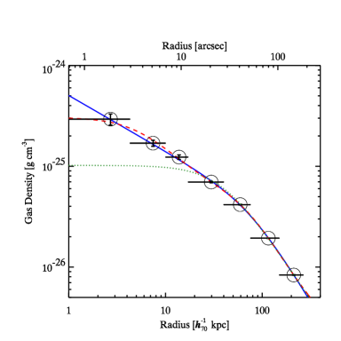
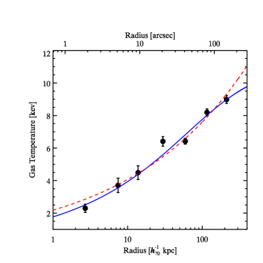
Figure 1: Left Panel: Chandra radial gas density profile of A2029. For clarity, large open circles are centered on the data points (the smallest error bars are difficult to see in the logarithmic scaling). Horizontal bars indicate the sizes of the annuli used to extract spectra, and the limits of the spherical shells in our de-projected analysis. Overlaid are the best-fitting cusp model (solid curve), single $\beta$-model (dotted curve), and double $\beta$-model (dashed curve). Right Panel: Chandra radial temperature profile of A2029. Overlaid are the best-fitting Bertschinger & Meiksin model (solid curve), and simple power-law model (dashed curve).

In Figure 1 we present the radial gas density and temperature data for A2029 (left and right panels, respectively). The horizontal bars indicate the widths of the annuli used, and are not error bars. Note the very small statistical errors in both $\rho_{g}$ and $T_{g}$, which indicate the precise spectral constraints obtained from these data. Since we wish to fit smooth, parameterized functions to the data (see below), we choose to assign an emission-weighted effective radius, $\bar{r}$, to each annulus $i$ (see, e.g., McLaughlin, 1999):

$$\bar{r}_{i}=[(r_{out_{i}}^{3/2}+r_{in_{i}}^{3/2})/2]^{2/3}.$$ (1)

While $\bar{r}$ should strictly be iteratively calculated from the fitted density profile, it is easy to show that eq. 1 is an excellent approximation to the correct $\bar{r}$ over the entire profile (e.g., Ettori et al., 2002a, see also §3.4).

3 Total Enclosed Mass Estimate

We make the assumptions of hydrostatic equilibrium and spherical symmetry, such that the enclosed mass is

$$M_{tot}(<\bar{r})=-{\frac{\bar{r}kT_{g}}{G\mu m_{p}}}\biggl{[}\frac{d{\rm ln}\rho_{g}}{d{\rm ln}r}+\frac{d{\rm ln}T_{g}}{d{\rm ln}r}\biggr{]},$$ (2)

where $k$ is Boltzmann’s constant, $G$ is the constant of gravitation, $\mu$ is the mean atomic weight of the gas (taken to be 0.62), and $m_{p}$ is the atomic mass unit. To obtain the instantaneous logarithmic derivatives necessary to evaluate eq. 2, we fit parameterized models to both the density and temperature. By parameterizing the $\rho_{g}$ and $T_{g}$ data we derive a mass profile that may be smoother than the true mass distribution. This approach, therefore, is best suited for interpreting average properties of $M(<r)$, such as its radial slope and comparison with DM simulations (also smooth), which are the focus of the present paper. Key advantages of this method are that it is simple to implement, and the mass profile is straightforward to interpret in terms of the input $\rho_{g}$ and $T_{g}$ profiles.

3.1 Temperature and Density Profiles

We initially fit the gas density data with the ubiquitous $\beta$-model:

$$\rho_{g}(r)=\rho_{g_{0}}[1+(r/r_{c})^{2}]^{-3\beta/2},$$ (3)

where $\rho_{g_{0}}$ is the central gas density, $r_{c}$ is the core radius, and $-3\beta$ is the slope of the profile at $r\gg r_{c}$. The result is overlaid on the data as a dotted curve (Fig. 1, left panel). Due to a peak in the profile at $<17$$h_{70}^{-1}$ kpc (the first 3 data points), the $\beta$-model does not provide an acceptable fit (see Table 3.1 below).

Table 3.1: Gas Density and Temperature Fits $\rho_{g}$-Model $(\chi^{2}$/dof) $\beta$ $r_{c}$[$\arcsec$] $\alpha_{\rho}$ cusp 6.6/3 $0.54\pm 0.01$ $53.4\pm 4.4$ $0.55\pm 0.03$ 1-$\beta$ 101.8/4 $0.48\pm 0.01$ $26.4\pm 1.1$  $\cdots$ 2-$\beta$ 2.0/1 $0.34\pm 0.37$ $3.7\pm 4.0$  $\cdots$ $0.76\pm 0.14$ $53.2\pm 9.5$  $\cdots$ $T_{g}$-Model $(\chi^{2}$/dof) $T_{\infty}$[keV] $r_{c}$[$\arcsec$] $\alpha_{T}$ B&M 14.3/4 $11.1\pm 1.6$ $122.1\pm 125.3$ $0.36\pm 0.05$ Power 19.8/5  $\cdots$ $\cdots$ $0.27\pm 0.01$

Table 1: Gas Density and Temperature Fits

Note.– For the cusp model, we find $\rho_{g_{c}}=6.6\pm 0.8\times 10^{-26}$g cm^-3. For the double-$\beta$ model, $\rho_{g1_{0}}=3.0\pm 0.5\times 10^{-25}$g cm^-3 and $\rho_{g2_{0}}=5.6\pm 1.8\times 10^{-26}$g cm^-3.

We explored two additional models: (1) the ‘cusp’ model, which is a modified $\beta$ model given by

$$\rho_{g}(r)=\rho_{g_{c}}2^{3\beta/2-\alpha_{\rho}/2}(r/r_{c})^{-\alpha_{\rho}}[1+(r/r_{c})^{2}]^{-3\beta/2+\alpha_{\rho}/2},$$ (4)

where $\rho_{g_{c}}\equiv\rho_{g}(r_{c})$, and the $\alpha_{\rho}$ parameter allows a steepening of the profile at $r<r_{c}$, and (2) a double-$\beta$ model (e.g., Xu et al., 1998; Mohr et al., 1999) given by

$$\rho_{g}(r)=\sqrt{\rho_{g1}^{2}+\rho_{g2}^{2}},$$ (5)

where $\rho_{g1}$ and $\rho_{g2}$ are each given by eq. 3.

The double-$\beta$ and cusp models both provide satisfactory fits to the data (dashed and solid curves, respectively, Figure 1, left panel), though the reduced $\chi^{2}$ is slightly improved for the double-$\beta$ model. We present the results of the gas density fits in Table 3.1. It is apparent that both the cusp and the double-$\beta$ models are sensitive to a break at $\approx 53\arcsec$, and that the parameters for the first component of the double-$\beta$ model are not well constrained. We have chosen the cusp model as our “reference” fit for the rest of our analysis for two reasons: (1) it provides a similar quality fit with two fewer free parameters than the double-$\beta$ model; (2) it yields a positive mass in the inner shell, which the $\beta$ models do not (see §3.4).

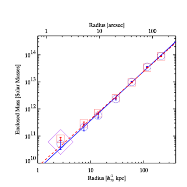
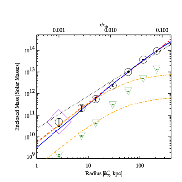
Figure 2: Left Panel: Total enclosed cluster mass, obtained from the B&M fit (open circles) and the power-law fit (open squares) to the temperature data. The cusp model for $\rho_{g}$ was used in both cases. Power-law fits to the mass points are overlaid on both data sets (solid line: B&M $T_{g}$ model, dashed line: power-law $T_{g}$ model). We have used large open symbols to identify the data points, as some of the error bars are barely visible in this logarithmic plot. The first data points are also enclosed with a large open diamond to emphasize the large additional systematic uncertainty at this radius (see §§3.2, 3.4). Right Panel: Total enclosed cluster mass (data points enclosed with open circles), overlaid with three different mass models: NFW (solid curve), power-law (dashed line), and M99 (dotted curve). The total enclosed gas mass is plotted as data points enclosed with open triangles. We have also overlaid an estimate of the stellar mass (dot-dashed curves, see §5.1). The lower curve assumes a $M_{*}/L_{V}$ of 1, the upper curve 12.

The temperature data are generally increasing, and are fairly well-fitted by a simple power-law $T(r)=Ar^{\alpha_{T}}$, with $\alpha_{T}=0.27\pm 0.01$ (overlaid as a dashed line). The power-law fit misses the central data point entirely, and predicts a steeply rising slope at the outer point. A somewhat better fit to the data is obtained with a Bertschinger & Meiksin (1986, B&M hereafter) profile (which adds an additional free parameter):

$$T(r)=T_{\infty}[r/(r+r_{c})]^{\alpha_{T}},$$ (6)

where $T_{\infty}$ is the asymptotic temperature at large radii. We have overlaid the two fitted models to the temperature data in Figure 1 (right panel). The B&M model (solid curve) provides an improvement in the fit to the data vs. the power-law model (dashed line) at the smallest and largest radii. The parameters of the fits are given in Table 3.1. From the table we see that the core radius is not well constrained, and that the temperature asymptotes to $11.1\pm 1.6$keV at large radii. Previous measurements of the temperature of A2029 at large radii (Molendi & De Grandi, 1999; White, 2000; Irwin & Bregman, 2001), indicate a gas temperature of $T_{g}\sim 5-8$ keV, suggesting a turnover in $T_{g}$ between $300-500$ $h_{70}^{-1}$ kpc. Future work incorporating data at larger radius will thus require a more sophisticated temperature model.

We note that as we found in Paper 1, the ICM of A2029 is apparently a single-phase gas at all radii. Even within a radius of $3\arcsec$, a single apec model provides an excellent fit to the data, and there is simply no spectral evidence to support an additional component such as a second temperature, a cooling flow model, or a power-law. The B&M model provides a very good approximation to the $T_{g}$ data except for underestimation of the fourth data point. We cannot determine if this is a statistical fluctuation, a systematic error in our analysis, or real structure in the $T_{g}$ profile. The last case would introduce a correction factor to the mass in that region, otherwise the temperature, and thus the mass profile appears quite smooth (see §3.4).

3.2 Mass Data and Fitted Profile

At each radius $i$, we have calculated the total enclosed gravitating mass $M(<\bar{r}_{i})$ according to eq. 2, using various density and temperature model fits. The logarithmic derivatives of $\rho_{g}$ and $T_{g}$ are evaluated at $\bar{r}_{i}$, and $T_{g}(\bar{r}_{i})$ is interpolated from the fitted $T_{g}$ model. We estimate statistical errors $\sigma_{M_{i}}$ on the mass data as follows: For each Monte Carlo simulation $j$ of the $\rho_{g}$ and $T_{g}$ data (§2.1), we obtain a pair of fitted profiles ($\rho_{fit_{j}}$ and $T_{fit_{j}}$) from which we calculate a set of mass values $M(<\bar{r}_{i})_{j}$. We thus obtain 100 mass values at each radius, from which we calculate the standard deviation and report it as the “1$\sigma$” error.

For the reference pair of gas models (the cusp model for $\rho_{g}$ and the B&M model for $T_{g}$), we present the total enclosed mass of A2029 in the left panel of Figure 2 (open circles). The profile has a nearly constant slope, with a slight flattening in the inner 3 data points. At our final data point, we obtain a total enclosed mass of $9.15\pm 0.25\times 10^{13}h_{70}^{-1}~{}{\rm M}_{\sun}$ within $260$$h_{70}^{-1}$ kpc. The mass calculated using the power-law $T_{g}$ model is also shown (open squares). We note that there is significant uncertainty in the mass at the innermost data point: while the temperature error is relatively high ($\sim 10\%$), the slopes of both $\rho_{g}$ and $T_{g}$ are even less well-constrained. In fact, using the double-$\beta$ model $\rho_{g}$ fit obtains a flat slope at this point, resulting in a negative mass value (see §3.4).

To analyze the shape of the mass profile, we fit parameterized models to the best fit mass values. To estimate errors on the parameters of these mass models, we obtain a mass fit $M_{fit_{j}}$ for each simulated mass data set $M(<\bar{r})_{j}$. As above, we therefore obtain 100 values of each parameter in a given mass model, from which we calculate a standard deviation. We have overlaid in Figure 2 (Left Panel) power-law fits to both mass profiles. The reference mass data are well-fitted by a power-law $M(<\bar{r})\propto r^{\alpha_{m}}$, with slope $\alpha_{m}=1.81\pm 0.04$ (solid line), over the entire mass range. The mass data obtained from using the power-law $T_{g}$ model are slightly higher below $r=17$$h_{70}^{-1}$ kpc, and are also well-fitted by a power-law with $\alpha_{m}=1.76\pm 0.03$ (dashed line).

Although the power-law is a good visual fit to the mass data, we have examined whether $\chi^{2}$ is reduced by instead using a broken power-law (BPL) model:

$$M(<r)=\begin{cases}A(r/r_{b})^{\alpha_{in}},&r<r_{b}\\ A(r/r_{b})^{\alpha_{out}},&r\geq r_{b}\end{cases}$$ (7)

where $r_{b}$ is the radius of the break between inner and outer slopes. If all the data points are included in the fit, then we obtain $r_{b}=5-14$ $h_{70}^{-1}$ kpc, with $\alpha_{in}=1.1-1.5$, and $\alpha_{out}$ consistent with $\alpha_{m}$ given above (these results assumed a cusp $\rho_{g}$ model, and either the B&M or power-law $T_{g}$ model). However, if the inner data point is excluded, then the BPL fits are consistent with the single power-law fits given above. Since the inner data point is subject to large systematic error due to the chosen $\rho_{g}$ parameterization (as above, see also §3.4), we can conclude there is no evidence for a significant break in the logarithmic radial mass profile.

To account for more gradual deviations from a power law, we have also fitted the mass data with the Navarro, Frenk, & White (1997, NFW hereafter) profile, $\rho(r)\propto[(r/r_{s})(1+(r/r_{s})^{2})]^{-1}$, the Hernquist (1990) model, $\rho(r)\propto[r(1+r)^{3})]^{-1}$, and the Moore et al. (1999, M99 hereafter) model, $\rho(r)\propto[(r/r_{s})^{1.5}(1+(r/r_{s})^{1.5})]^{-1}$. Integrating these density profiles obtains mass models for fitting; analytic forms can be found in the literature (see, e.g., Klypin et al., 2001; Loewenstein & Mushotzky, 2002). These fits are presented in the next section.

3.3 The Dark Matter Distribution

Assuming the cluster to be dominated by DM (a point we argue below), the fitted total mass profile corresponds to an implicit DM density distribution. For any power-law fit, $\rho_{DM}\propto r^{\alpha_{DM}}$, where $\alpha_{DM}=\alpha_{m}-3$. For the power-law fit to the reference mass profile we therefore observe a dark matter density slope of $\alpha_{DM}=-1.19\pm 0.04$.

In Figure 2, (right panel) we again show the total enclosed mass profile (open circles). To compare with other clusters, as well as theoretical expectations, it is convenient to scale the radius in terms of the virial radius, $r_{\rm{vir}}$. We calculate one popular predicted value of $r_{\rm{vir}}$ as a function of emission-weighted global temperature, using the form given by Neumann & Arnaud (1999), eq. 9, normalized to the 2.0-9.5 keV band Mass-Temperature relation given by Mathiesen & Evrard (2001), which we convert to our cosmology. If we extract one spectrum in this band from the entire region within $186\arcsec$ which we observe with Chandra, we measure a single-temperature fit of $7.54\pm 0.15$ keV. We thus obtain $r_{\rm{vir}}=2.71\pm 0.42$$h_{70}^{-1}$ Mpc for A2029. We have plotted the upper axis of Fig. 2 (right panel) in units of $r_{\rm{vir}}$, which shows that we are examining the dark matter profile on a scale from $<0.001-0.1r_{\rm{vir}}$.

We have overlaid fits to the mass profile of A2029 from three different mass models: a power-law (dashed line), an NFW mass model (solid curve), and an M99 model (dotted curve). While the power-law model provides a good overall fit ($\chi^{2}$/dof $=24.1/5$), the NFW model is preferred ($\chi^{2}$/dof $=11.8/5$). The data are more closely approximated by the NFW profile except for a $\sim 1.5\sigma$ difference at the innermost data point, which has additional systematic uncertainties (as noted above) rendering the discrepancy insignificant (see §3.4). The Hernquist profile fit (not shown) is nearly identical to the NFW fit ($\chi^{2}$/dof $=11.4/5$). The M99 model does not provide an acceptable fit to the overall profile ($\chi^{2}$/dof $=250.1/5$), though its small radius slope is compatible with the inner 3 data points. However, if fit solely to these points, it falls well below the remainder of the mass profile, which is better constrained. We note that although the NFW and Hernquist models improve $\chi^{2}$ significantly, the relative differences between these models vs. the power-law mass model are small ($<10\%$ between 17 and 260 $h_{70}^{-1}$ kpc). Unlike the BPL model, which presents a sharp break, the gradual change in the logarithmic slope of the NFW or Hernquist profiles better quantifies the small deviations of the mass data from a pure power-law.

For the NFW profile, we find a scale radius $r_{s}=540\pm 90$$h_{70}^{-1}$ kpc, and a concentration parameter $c=4.4\pm 0.9$. This allows us to calculate the value of $r_{\rm{vir}}$ expected from the NFW model ($r_{\rm{vir}}\equiv cr_{s}$), for which we obtain $r_{\rm{vir}}$(NFW)$=2.39\pm 0.62$$h_{70}^{-1}$ Mpc, in good agreement with $r_{\rm{vir}}$ as predicted by the Mass-Temperature relation given above.

Several other authors find that CDM halos (e.g., NFW or M99 profiles) are also consistent with their X-ray cluster observations at $r\gtrsim 0.1r_{\rm{vir}}$ (e.g., Ettori et al., 2002b; Pratt & Arnaud, 2002; Schmidt et al., 2001; Allen et al., 2001; Arabadjis et al., 2002), while gravitational lensing studies report conflicting results in cluster cores (i.e., Sand et al., 2002; Natarajan et al., 2002). The Hydra A cluster exhibits $\rho_{DM}\propto r^{-1.3}$ over a similar range of radii to our analysis (David et al., 2001), however, there are prominent interactions between the X-ray gas and the radio source in that system, implying significant deviations from hydrostatic equilibrium. Thus the DM profile inferred for A2029 (which is comparatively undisturbed in this regime), provides evidence that the Hydra A results are robust, and is an important independent confirmation of CDM predictions.

3.4 Possible Systematic Errors in the Mass Profile

We have explored several alternative data reduction and analysis choices to investigate systematic errors in the mass profile. We have calculated density, temperature and mass profiles in four different sets of annuli: (1) the original 11 annuli used in Paper 1, (2) 13 annuli, obtained by dividing the inner 2 annuli of Paper 1 into 4 smaller annuli, (3) 5 annuli, using much larger bins, (4) 7 annuli, using a combination of the very small annuli from (2) in the center with the larger, higher S/N annuli from (3). Binning choice (4) is the reference choice for this paper, which shows the most detail in the core, and provides the highest S/N for the temperature estimates at larger radii. For all 4 choices of binning, the resulting mass profiles are not perceptibly different from the reference results. We have also analyzed the data in energy ranges of $0.5-8.0$, $0.7-8.0$, and $1.0-8.0$ keV, and repeated the entire experiment using a MEKAL plasma model rather than the APEC reference model; in all cases the slope of the fitted mass profile is within the $1\sigma$ errors of the reference fit.

The effect on the mass profile of our choice of eq. 1 to calculate $\bar{r}$ can be tested by instead using 2 extreme cases for the estimate of $\bar{r}$: assumed density slopes of $\rho_{g}\propto r^{0}$ and $\propto r^{-3}$, which easily bracket all the instantaneous slopes of the observed density profile (see also Ettori et al., 2002b). We find that the mass profile does not vary perceptibly with the choice of $\bar{r}$.

Our reference analysis is to use the same Period C background files as in Paper 1. Variations in the X-ray flux of the extragalactic sky between our target and the background templates may render them inaccurate. We experimented with modifying the background flux by changing the effective exposure time of the templates to $\pm 20\%$ of its nominal value. While this can affect the estimated temperature in the outermost annulus, the overall temperature profile does not vary beyond the $1\sigma$ errors, nor does the slope of the mass profile. We have corrected the data using the “corrarf” routine (§2), which results in lower $T_{g}$ values than we reported in Paper 1, by up to 16% in the outermost bin. This has the effect of slightly flattening the fitted $T_{g}$ profile, as well as the mass profile (the uncorrected profile has overall slope $\alpha_{m}=1.91\pm 0.03$). The calibration of the ACIS instrument below 1 keV is ongoing, but it is reportedly now accurate at the $\approx 10\%$ level (see footnote 3).

In Figure 2 (Left Panel) we show the total mass values obtained from each of the two temperature profiles shown in Figure 1 (in both cases, we use the cusp fit to $\rho_{g}$). The mass values all overlap in their $1\sigma$ error bars, as do the slopes of the mass profiles. We have also explored the choice of the model which is fit to $\rho_{g}$. The overall power-law fits to the mass profiles derived from the cusp and double-$\beta$ profiles are indistinguishable. However, we note that the double-$\beta$ model results in a negative (and unphysical) mass value in the central bin (due to its large statistical uncertainty, it does not affect the overall profile fit). The single $\beta$ model (which is an unacceptable fit to the $\rho_{g}$ data) also obtains a very flat slope for the inner 3 data points which results in negative mass values over that region. To obtain a positive mass, eq. 2 requires a negative sum for the logarithmic derivatives: inspection of Figure 1 shows that the slopes of neither $\rho_{g}$ nor $T_{g}$ are well-constrained at the radius of the innermost data point. The cusp and double-$\beta$ models diverge in this regime, but the data do not distinguish between them. If the gas was in fact isothermal at this radius our mass estimate would be positive for all 3 $\rho_{g}$ fits, but without much higher S/N data (at higher spatial resolution) we cannot infer such a state for the gas. We note that exclusion of the innermost data point has no perceptible affect on the mass profile fit.

The use of parameterized functions for $\rho_{g}$ and $T_{g}$ has the effect of smoothing those data, in turn resulting in a smoother mass profile (§3.1). We have also calculated the mass profile by using a simple “point-to-point” estimation of the $\rho_{g}$ and $T_{g}$ slopes where the logarithmic derivatives needed for eq. 2 are taken to be the slope between each pair of adjacent points. The mass values are significantly different only in the fourth and fifth bins, which lie above and below the reference data points, respectively. Nonetheless, the average slope of the mass profile is not altered beyond the $1\sigma$ limits of the reference fit (as one would expect, since the reference $\rho_{g}$ and $T_{g}$ models provide good fits to the data). Aside from the innermost data point, the slopes of $\rho_{g}$ and $T_{g}$ are well constrained regardless of the parameterization, and the overall mass profile is robust.

We have assumed spherical symmetry for A2029, though its mass distribution exhibits an average ellipticity of 0.5 (Buote & Canizares, 1996) within $\approx 1.6$$h_{70}^{-1}$ Mpc inferred from the X-rays and optical light. However, we have measured the spherically averaged mass distribution, which is quite insensitive to the ellipticity of the system (including the specific case of A2029, Buote & Canizares 1996; see also Evrard et al. 1996). This approach is also useful for comparison with simulations which also present a spherically averaged profile (i.e., NFW, M99).

4 Gas Mass, Baryon Fraction, and $\Omega_{m}$

We have calculated the total gas mass $M_{gas}(\bar{r})$ in each spherical shell directly and summed them to obtain an enclosed gas mass profile (i.e., we do not interpolate the $\rho_{g}$ values from the fitted profile as we did for $T_{g}$ in the total mass calculation; the results with either method are unchanged). In Figure 2 (Right Panel) we have overlaid the total enclosed gas mass profile (open diamonds). We see that the gas mass at the center of the cluster is $<3\%$ of the total mass, rising to $13.9\pm 0.4\%$ at our last measured data point. This may safely be regarded as a lower limit, as simulations and other measurements suggest a higher asymptotic value for the gas mass fraction in clusters, f${}_{gas}(r_{\rm{vir}})\sim 0.2-0.3h_{70}^{-3/2}$ (e.g., Allen et al., 2002), while we only have observations at $r\leq 0.1r_{\rm{vir}}$.

Assuming that A2029 contains proportions of dark matter and baryonic matter equal to their Universal values, one may place an upper limit on $\Omega_{m}$ with f_gas. Given the Universal baryon mass density from big bang nucleosynthesis calculations and recent observations of the deuterium abundance ($\Omega_{B}$(BBN)), one finds $\Omega_{m}=\Omega_{B}\rm{(BBN)}/{\rm{f}}_{B}$, where f_B is the Universal baryon mass fraction. Given $\Omega_{B}h^{2}\rm{(BBN)}=0.020\pm 0.001$ (see, e.g., Burles et al., 2001), $h=0.7\pm 0.07$, and f${}_{B}\geq$ f${}_{gas}\geq 0.139\pm 0.004h_{70}^{-3/2}$ from this work, we estimate $\Omega_{m}\leq 0.29\pm 0.03h_{70}^{-1/2}$, in agreement with current estimates (for a recent review, see Turner, 2002).

5 Mass Budget of the Core

Massive elliptical galaxies such as NGC 720 (Buote et al., 2002a), and NGC 4636 (Loewenstein & Mushotzky, 2002), are apparently DM-dominated all the way into their cores. This situation is likely to exist in a cD cluster such as A2029, except at possibly the smallest scales ($r\approx 1-10$kpc), where the cD stellar mass component may be more important (Dubinski, 1998). We have found that the gas in A2029 is only a few percent of the total mass in the core of the system. But are we observing the stellar mass (e.g., the cD)? Dubinski suggests the turnover between stellar and DM-domination should occur at a few tens of kpc; but although we are specifically observing this regime, we see no significant break in the mass profile (see §3.2). The outlying fourth $T_{g}$ point and the central $\rho_{g}$ peak over a single $\beta$-model are intriguing, but the balance of the data suggest that any transition from stellar-dominated to DM-dominated regimes is quite smooth in this system.

5.1 Stellar Mass

We have estimated the contribution of stellar matter to the system, by using optical observations of the cD galaxy in A2029 and its diffuse halo. Uson et al. (1991) conducted a detailed optical analysis of A2029, and observed that the surface brightness of the cD+halo was well-fitted by a de Vaucouleurs (1948) profile out to $\approx 300\arcsec$. They report a total $R$-band luminosity of $5\times 10^{11}h^{-2}_{100}{\rm L}_{\sun}$ for the cD+halo, which is 41% of the total light of the cluster within $260\arcsec$ radius. We assume the cD+halo to be the vast majority of the light within its effective radius $R_{e}=52\arcsec$ (76$h_{70}^{-1}$ kpc). Using the Hernquist (1990) model as an approximate deprojection of the $R^{1/4}$ law, we normalize to the total light of Uson et al. (1991), converting to our cosmology, and the $V$ band, and obtain a luminosity profile. In Figure 3, we present the total cluster mass-to-light ratio ($M_{tot}/L_{V}$) profile of the core of A2029, based on the cD+halo light profile. It is consistent with a constant $M_{tot}/L_{V}\approx 12{\rm M}_{\sun}/{\rm L}_{\sun}$ within 20$h_{70}^{-1}$ kpc, and rises rapidly at larger radius.

Figure 3: Ratio of total enclosed cluster mass to stellar light from the cD and diffuse envelope in A2029. The light follows an $R^{1/4}$ law with $R_{e}=52\arcsec$, which we have approximated by a Hernquist (1990) profile normalized to a total cD+envelope $R$-band luminosity of $5\times 10^{11}h^{-2}_{100}\rm{L}_{\sun}$ (Uson et al., 1991), converted to our cosmology and the $V$-band. Error bars represent the uncertainty in the mass estimate.

Dynamical stellar analyses estimate the total masses of galactic systems, but cannot directly measure the stellar mass. Attempts to resolve this with population synthesis techniques yield highly uncertain results for the stellar mass-to-light ratio, $M_{*}/L_{V}=1-12{\rm M}_{\sun}/{\rm L}_{\sun}$ (Pickles, 1985). Using these bounding values for $M_{*}/L_{V}$ we plot in Figure 2 (right panel) associated stellar mass profiles (dot-dashed curves) for the cD+halo system. The data indicate that at $r<0.005r_{\rm{vir}}$ ($\approx 15$$h_{70}^{-1}$ kpc) the stellar mass can potentially dominate the system, depending on the highly uncertain assumed $M_{*}/L_{V}$. The stellar material outweighs the gas mass up to a radius between $\approx 0.005-0.04r_{\rm{vir}}$ ($\approx 15-100$$h_{70}^{-1}$ kpc). If we assert a plausible value, $M_{*}/L_{V}=5~{}{\rm M}_{\sun}/{\rm L}_{\sun}$ for the system, we would conclude that the cluster is DM dominated down to the smallest scales measured here, which is consistent with a single NFW mass component (and also with the lack of a significant break in the total mass profile, §3.2). Alternatively, the gas density peak over the $\beta$-model at $r<17$$h_{70}^{-1}$ kpc, or the outlying $T_{g}$ data point may indicate the presence of a stellar mass component in excess of (or differing from) an NFW DM halo.

5.2 Velocity Dispersion

An interesting comparison can be made with the optical velocity dispersion profile of A2029. As noted by Dubinski (1998), IC1101 (the cD galaxy in A2029) is one of the only brightest cluster galaxies observed to have an increasing velocity dispersion, $\sigma_{V}$, (Dressler, 1979). We may regard the stars in the cD galaxy (from which $\sigma_{V}$ is measured) to be simply another family of tracer particles (as the hot ICM gas particles) bound to the same gravitational potential.

Thus, the effective velocity of the ICM gas particles may be expected to mirror that of the stars. We estimate the velocity dispersion for the ICM gas as $\sigma_{ICM}^{2}=kT_{g}/\mu m_{p}$. The temperature data yield $\sigma_{ICM}^{2}\propto r^{0.27\pm 0.01}$, while the cD velocity dispersion profile of Dressler (1979), measured over the range $2-100h_{50}^{-1}$ kpc reveals $\sigma_{V}^{2}\propto r^{0.25}$. This correspondence is not required for the condition of hydrostatic equilibrium, but the similarity of the two species is striking. A2029 is one of the few systems where the shape of both the X-ray and optical velocity dispersions can be measured in detail: the consistency between them is further evidence that we are observing a dynamically relaxed system where all the mass components are in equilibrium with the gravitational potential.

6 Conclusions

We have analyzed high spatial resolution Chandra data of the A2029 cluster of galaxies, obtaining well-constrained ICM gas density and temperature profiles on scales of $0.001-0.1r_{\rm{vir}}$ ($\approx 3-260$$h_{70}^{-1}$ kpc). Fitting smooth functions to these profiles, we obtain mass profiles for A2029, measuring the shape of the total mass profile at unprecedented accuracy to a very small fraction of the virial radius. Our results are insensitive to most details of the data reduction, but are closely tied to the well-constrained temperature and density distributions.

We find that the shape of the inferred dark matter density at $<0.1r_{\rm{vir}}$ is consistent with the NFW parameterization of CDM halos, but apparently incompatible with that of M99, though we note that individual objects may be expected to show significant scatter from a mean DM halo profile (Bullock et al., 2001).

The consistency of the NFW model with the mass profile all the way down to $<0.01r_{\rm{vir}}$ indicates that there is no need to modify the standard CDM paradigm to fit the DM distribution in this cluster, consistent with X-ray observations of other clusters at larger radii (see §3.3). This result contrasts with the strong deviations from the CDM predictions observed in the rotation curves of low surface brightness galaxies (e.g., Swaters et al., 2000), and dwarf galaxies (e.g., Moore et al., 1999) which inspired the self-interacting DM model (Spergel & Steinhardt, 2000) to explain the relatively flat core density distributions in these galaxies. Hence in light of the good agreement with the NFW profile in clusters, the deviations observed on small galaxy scales do not seem to imply a fundamental problem with the general CDM paradigm. Instead, it is likely that the numerical simulations do not currently account properly for the effects of feedback processes on the formation and evolution of small halos.

Our analysis suggests that A2029 is dominated by a single mass (i.e., DM) component at all measured scales below $0.1r_{\rm{vir}}$, or that any transition from a stellar mass dominated component in the cD and a DM component is quite gradual. We also observe a rising gas fraction from $<3\%$ to $>14\%$ in A2029, obtaining an upper limit to $\Omega_{m}\leq 0.29\pm 0.03h_{70}^{-1/2}$, consistent with other current studies.

References

- Allen et al. (2001) Allen, S. W., Schmidt, R. W., & Fabian, A. C. 2001, MNRAS, 328, L37
- Allen et al. (2002) —. 2002, MNRAS, 334, L11
- Arabadjis et al. (2002) Arabadjis, J. S., Bautz, M. W., & Garmire, G. P. 2002, ApJ, 572, 66
- Bertschinger & Meiksin (1986) Bertschinger, E. & Meiksin, A. 1986, ApJ, 306, L1
- Briel & Henry (1994) Briel, U. G. & Henry, J. P. 1994, Nature, 372, 439
- Bullock et al. (2001) Bullock, J. S., Kolatt, T. S., Sigad, Y., Somerville, R. S., Kravtsov, A. V., Klypin, A. A., Primack, J. R., & Dekel, A. 2001, MNRAS, 321, 559
- Buote (2000) Buote, D. A. 2000, ApJ, 539, 172
- Buote & Canizares (1996) Buote, D. A. & Canizares, C. R. 1996, ApJ, 457, 565
- Buote et al. (2002a) Buote, D. A., Jeltema, T. E., Canizares, C. R., & Garmire, G. P. 2002a, ApJ, 577, 183
- Buote et al. (2002b) Buote, D. A., Lewis, A. D., Brighenti, F., & Mathews, W. G. 2002b, ApJ, submitted (astro-ph/0205362)
- Buote & Tsai (1996) Buote, D. A. & Tsai, J. C. 1996, ApJ, 458, 27
- Burles et al. (2001) Burles, S., Nollett, K. M., & Turner, M. S. 2001, ApJ, 552, L1
- Dahle et al. (2002) Dahle, H., Hannestad, S., & Sommer-Larsen, J. 2002, ApJL, submitted (astro-ph/0206455)
- Davé et al. (2001) Davé, R., Spergel, D. N., Steinhardt, P. J., & Wandelt, B. D. 2001, ApJ, 547, 574
- David et al. (2001) David, L. P., Nulsen, P. E. J., McNamara, B. R., Forman, W., Jones, C., Ponman, T., Robertson, B., & Wise, M. 2001, ApJ, 557, 546
- de Grandi & Molendi (1999) de Grandi, S. & Molendi, S. 1999, ApJ, 527, L25
- De Grandi & Molendi (2002) De Grandi, S. & Molendi, S. 2002, ApJ, 567, 163
- de Vaucouleurs (1948) de Vaucouleurs, G. 1948, Annales d’Astrophysique, 11, 247
- Dressler (1979) Dressler, A. 1979, ApJ, 231, 659
- Dubinski (1998) Dubinski, J. 1998, ApJ, 502, 141
- Ettori et al. (2002a) Ettori, S., De Grandi, S., & Molendi, S. 2002a, A&A, 391, 841
- Ettori et al. (2002b) Ettori, S., Fabian, A. C., Allen, S. W., & Johnstone, R. M. 2002b, MNRAS, 331, 635
- Evrard et al. (1996) Evrard, A. E., Metzler, C. A., & Navarro, J. F. 1996, ApJ, 469, 494
- Fabian et al. (2002) Fabian, A. C., Celotti, A., Blundell, K. M., Kassim, N. E., & Perley, R. A. 2002, MNRAS, 331, 369
- Girardi et al. (2002) Girardi, M., Manzato, P., Mezzetti, M., Giuricin, G., & Limboz, F. . 2002, ApJ, 569, 720
- Hernquist (1990) Hernquist, L. 1990, ApJ, 356, 359
- Irwin & Bregman (2000) Irwin, J. A. & Bregman, J. N. 2000, ApJ, 538, 543
- Irwin & Bregman (2001) —. 2001, ApJ, 546, 150
- Johnstone et al. (2002) Johnstone, R. M., Allen, S. W., Fabian, A. C., & Sanders, J. S. 2002, MNRAS, 336, 299
- Klypin et al. (2001) Klypin, A., Kravtsov, A. V., Bullock, J. S., & Primack, J. R. 2001, ApJ, 554, 903
- Lewis et al. (2002) Lewis, A. D., Stocke, J. T., & Buote, D. A. 2002, ApJ, 573, L13 (Paper 1)
- Loewenstein & Mushotzky (2002) Loewenstein, M. & Mushotzky, R. F. 2002, ApJ, submitted (astro-ph/0208090)
- Markevitch et al. (1998) Markevitch, M., Forman, W. R., Sarazin, C. L., & Vikhlinin, A. 1998, ApJ, 503, 77
- Markevitch et al. (2000) Markevitch, M., Ponman, T. J., Nulsen, P. E. J., Bautz, M. W., Burke, D. J., David, L. P., Davis, D., Donnelly, R. H., Forman, W. R., Jones, C., Kaastra, J., Kellogg, E., Kim, D.-W., Kolodziejczak, J., Mazzotta, P., Pagliaro, A., Patel, S., Van Speybroeck, L., Vikhlinin, A., Vrtilek, J., Wise, M., & Zhao, P. 2000, ApJ, 541, 542
- Markevitch et al. (2002) Markevitch, M., Vikhlinin, A., & Forman, W. R. 2002, ASP Conf. Ser., in press (astro-ph/0208208)
- Markevitch et al. (1999) Markevitch, M., Vikhlinin, A., Forman, W. R., & Sarazin, C. L. 1999, ApJ, 527, 545
- Mathiesen et al. (1999) Mathiesen, B., Evrard, A. E., & Mohr, J. J. 1999, ApJ, 520, L21
- Mathiesen & Evrard (2001) Mathiesen, B. F. & Evrard, A. E. 2001, ApJ, 546, 100
- Matsushita et al. (2002) Matsushita, K., Belsole, E., Finoguenov, A., & Böhringer, H. 2002, A&A, 386, 77
- McLaughlin (1999) McLaughlin, D. E. 1999, AJ, 117, 2398
- Mohr et al. (1999) Mohr, J. J., Mathiesen, B., & Evrard, A. E. 1999, ApJ, 517, 627
- Molendi & De Grandi (1999) Molendi, S. & De Grandi, S. 1999, A&A, 351, L41
- Moore et al. (1999) Moore, B., Quinn, T., Governato, F., Stadel, J., & Lake, G. 1999, MNRAS, 310, 1147
- Natarajan et al. (2002) Natarajan, P., Loeb, A., Kneib, J., & Smail, I. 2002, ApJ, 580, L17
- Navarro et al. (1997) Navarro, J. F., Frenk, C. S., & White, S. D. M. 1997, ApJ, 490, 493
- Neumann & Arnaud (1999) Neumann, D. M. & Arnaud, M. 1999, A&A, 348, 711
- Nulsen & Bohringer (1995) Nulsen, P. E. J. & Bohringer, H. 1995, MNRAS, 274, 1093
- Nulsen et al. (2002) Nulsen, P. E. J., David, L. P., McNamara, B. R., Jones, C., Forman, W. R., & Wise, M. 2002, ApJ, 568, 163
- Pickles (1985) Pickles, A. J. 1985, ApJ, 296, 340
- Pratt & Arnaud (2002) Pratt, G. W. & Arnaud, M. 2002, A&A, 394, 375
- Sand et al. (2002) Sand, D. J., Treu, T., & Ellis, R. S. 2002, ApJ, 574, L129
- Schmidt et al. (2001) Schmidt, R. W., Allen, S. W., & Fabian, A. C. 2001, MNRAS, 327, 1057
- Spergel & Steinhardt (2000) Spergel, D. N. & Steinhardt, P. J. 2000, Physical Review Letters, 84, 3760
- Swaters et al. (2000) Swaters, R. A., Madore, B. F., & Trewhella, M. 2000, ApJ, 531, L107
- Townsley et al. (2000) Townsley, L. K., Broos, P. S., Garmire, G. P., & Nousek, J. A. 2000, ApJ, 534, L139
- Tsai et al. (1994) Tsai, J. C., Katz, N., & Bertschinger, E. 1994, ApJ, 423, 553
- Turner (2002) Turner, M. S. 2002, ApJ, 576, L101
- Uson et al. (1991) Uson, J. M., Boughn, S. P., & Kuhn, J. R. 1991, ApJ, 369, 46
- White (2000) White, D. A. 2000, MNRAS, 312, 663
- Xu et al. (1998) Xu, H., Makishima, K., Fukazawa, Y., Ikebe, Y., Kikuchi, K., Ohashi, T., & Tamura, T. 1998, ApJ, 500, 738