The Carlsberg Meridian Telescope CCD Drift Scan Survey

This paper contains the general data reduction methods used in processing the data from the Carlsberg Meridian Telescope CCD Drift Scan Survey. An efficient method to calibrate the fluctuations in the positions of the images caused by atmospheric turbulence is described. The external accuracy achieved is 36 mas in right ascension and declination. A description of the recently released catalogue is given.

1 Introduction

The Carlsberg Meridian Telescope (CMT) has recently undergone a major upgrade. A 2k by 2k CCD camera has been installed with a Sloan $r^{\prime}$ filter operating in a drift scan mode. With the new system, the effective exposure time is about 90s, the magnitude limit is $r^{\prime}_{\rm CMT}=$17 and the initial positional accuracy is in the range 0.05^′′ to 0.10^′′.

The main task of the CMT is to map the sky in the declination range $-$3$\degr$ to $+$30$\degr$ with the aim of providing an astrometric, and photometric, catalogue that can accurately transfer the Hipparcos/Tycho reference frame to Schmidt plates. A secondary survey is also planned that extends the declination range covered to $-$15$\degr$ in the South and $+$50$\degr$ in the North. Projects similar to the CMT (UCAC, Zacharias et al. (2000) and CMASF, Muiños et al. (1998)), which include the Southern hemisphere, will also be able to provide astrometric calibration for VISTA and other deep wide-field surveys.

The two main systematic errors affecting the data are caused by image motions due to long timescale atmospheric turbulence and charge transfer efficiency (CTE) problems linked to the CCD. Methods are described on how to calibrate these errors.

2 The telescope system

The telescope is a Grubb Parsons refractor with an objective of 178 mm diameter and focal length 2.66 m. After initially being located at Brorfelde, Denmark, the telescope was moved in 1984 to La Palma in the Canary Islands to take advantage of the better observing conditions there.

Originally, the detector used was a scanning-slit photoelectric micrometer, but was replaced in 1998 by a CCD camera operating in a drift scan mode. This was a major change in the method of observing, since relative astrometry with respect to a dense grid of standards within the same data frames would be used rather than absolute astrometry and offsetting the telescope with respect to the standards.

The two significant advantages of a CCD system are that fainter stars can be observed and that many stars can be observed simultaneously. This has increased the number of stars that can be observed in a night by a factor of more than 100. However, there is a disadvantage with the new system in that close to the celestial pole the images become distorted. This is discussed further in Section 4.4. Although this restricts normal observing to declinations South of $+60\degr$, it is more than compensated by the amount of high-quality data that it produces.

More recently (April 1999) the CCD system was upgraded to a larger detector (Kodak 2k$\times$2k with 9$\mu$m pixels) and a filter equivalent to the Sloan Digital Sky Survey $r^{\prime}$ passband was fitted.

The increase in the CCD size has a number of advantages which include: completing the survey faster due to a larger field of view; providing a deeper survey due to longer exposures; and improvements in the calibration due to increased frame sizes. Also, with the fitting of the $r^{\prime}$ filter, the project is now also able to provide photometry on a commonly-used photometric system.

The new CCD pixel size corresponds to $0.7^{\prime\prime}$ and considering that the median seeing at the telescope is just under $3^{\prime\prime}$ the images are well sampled. It should be noted that the site seeing is much better than this.

The CCD can be cooled to $-65\degr$C by a Peltier cooler. Currently, the chip is cooled to $-30\degr$C since this reduces the effect of a charge transfer efficiency (CTE) problem with the chip (see Appendix A). The higher operating temperature does not affect our magnitude limit.

These improvements with the CCD and the new filter have increased the number of stars observed by about 4 times as many stars per night than with the old CCD system. The current magnitude limit is $r^{\prime}_{\rm CMT}=17$ and between 100,000 and 200,000 stars a night are observed. On a typical night, more than 50 square degrees are covered.

More details about the telescope can be found in Helmer & Morrison (1985) and about the recent upgrades in Evans 2001b . A summary is given in Table 1.

Table 1: A summary of the telescope and camera parameters for the current configuration.

Telescope:	Located on La Palma, Canary Islands
	178 mm objective
	2.66 m focal length
Camera:	CCD chip – Kodak (KAF-4202 Grade:C1)
	2060$\times$2048 pixels
	Pixel size 9$\mu$m (0.7′′)
	CUO built
	Operating temperature $-$30$\,\degr$C
System:	Automatic and remotely controlled
	Drift scans
	(generates $\sim$3 Gb of data per night)
	Data automatically parameterized
	(reduced to 6-7 Mb)
	Daily reductions take about 30 min.
	100,000–200,000 stars observed per night
	Calibrated with respect to Tycho 2
	Magnitude limit (Sloan) $r^{\prime}_{\rm CMT}=$17

3 Observing strategy

The effective width of the CCD is 2060 pixels which corresponds to drift scans of width $23^{\prime}$. The selection of where to observe is constrained by the survey nature of the current project. Since specific objects are not the targets, the observing is carried out at evenly spaced declinations (every $0.25\degr$). This allows for a uniform overlap of $8\,^{\prime}$ in declination between scans, which provides enough data to quantify the difference between two adjacent frames and calibrate the atmospheric fluctuations (see Section 4.3).

Each day preliminary calibrations are carried out which provide quality control information which is then fed into the observation selection programme. The basic principle of the selection programme is to maximize the lengths of the observations. The reason for doing this is to minimize the number of intervals between observations during which the telescope is moving to a new declination and the CCD is being read out and thus maximize the amount of time collecting data.

Various declination zones have different priorities, so that the primary survey area ($-$3$\degr$ to $+$30$\degr$ declination) is completed before other areas are observed. Additionally, a $20^{\circ}$ zone of avoidance around the Moon is used. There is also a minimum observation length of 20 minutes, otherwise the Tycho 2 preliminary calibration will probably fail due to too few standards being available. A typical drift scan lasts about an hour, although exposures up to 5 hours have been made.

Additional calibrations are carried out off-line at Cambridge in order to account for the CTE and atmospheric fluctuation problems. From these it is possible to identify further problem data frames that need to be reobserved. This information is then fed back to the selection programme after the calibrations have been visually inspected.

4 Astrometric data reductions

In this section the main astrometric data reduction is discussed. The data from the CCD is reduced automatically as soon as the observation has been completed. The data reduction system automatically detects and parameterizes images and produces other data monitoring diagnostics. During the day, the observer then carries out a preliminary calibration which serves both as a first pass calibration and also as a quality control check. Most of the analysis for systematic effects is carried out on the data at this stage. Finally, the data is accumulated and a catalogue formed.

4.1 Image Analysis

The data processing pipeline is designed to ingest the variable-length drift scan two-dimensional images and automatically detect and parameterize objects located on the frames. The nature of the remote operation precluded long term storage of the drift scan images ($\sim$3 Gbytes/night) and correspondingly defined the automated nature of the processing pipeline. By storing only relevant information (position, intensity, shape) for each detected object, a factor of $\sim$100 compression over the raw data results, with virtually no loss of relevant information. The resulting object catalogues then form the basis of all subsequent reductions. Generic data quality control information is also extracted from the pipeline products and contributes to monitoring the health of the overall system.

As usual, the first part of the data processing involves removing the instrumental signature, which in this case reduces to a one-dimensional correction perpendicular to the drift scan direction. In theory, with a modern CCD camera, these corrections involve correcting for the DC bias level and then flatfielding out the remaining systematic effects. However, in practice, we found that the additive bias correction was not simply a constant level across the frame and indeed was difficult to disentangle from the effects of the multiplicative flatfield correction. After a series of on-sky tests (see Appendix B) we found that the dominant contribution to background variations across the scan direction was additive in nature and that after correcting for this no significant flatfield variations (ie. $\gtrsim$1%) remained.

Consequently, the first pass preprocessing consists of using the underscan and overscan regions to monitor the overall bias (or zero) level of the device, while the active part of the CCD defines the differential additive correction to be applied in subsequent processing stages. We suspect the control and readout electronics introduce the varying (but repeatable over intervals $\approx$nightly) bias level across the CCD rows during clocking out each row of data. The bias correction is defined as the median of the data in each column with respect to the median level of the underscan and overscan regions.

In the same pass through the data, the general one-dimensional background variation down the scan direction (ie. as a function of RA/time) is also recorded, again using the median level, with an effective scale length of $\sim$ 1 arcmin. At the same time as the background variation is monitored, a robust estimate of the rms sky noise is made based on the Median of the Absolute Deviations from the median (MAD estimator - see Hoaglin, Mosteller, & Tukey 1983 for more details). Finally, an overall estimate of the sky noise level for the whole frame is made from the median of the MAD estimates.

In normal conditions, the sky is sufficiently uniform over the cross-scan direction and at such a low level ($\approx$10 counts cf. readout noise of 7 counts) that tracking its variation in the scan direction is sufficient. All bias and sky level estimates are saved for subsequent diagnostic and data quality control checks.

On the second, and final, pass the background-corrected data is then searched for discrete astronomical objects using the techniques described by Irwin (1985, 1996). Briefly, this consists of using a matched isophotal detection algorithm to locate regions of connected pixels above a definable detection threshold (typically 1.5 $\times$ sky noise level). Each such region defines a potential astronomical object, which may be single or multiple. The contiguous pixel lists are then searched for the presence, or otherwise, of multiple components. The flux is appropriately partitioned, if needed, and various image parameters describing the location, intensity and shape are computed (see Irwin (1996)).

Since the primary driver of the project is the astrometric precision attainable, the choice of image parameterization method was dominated by this consideration coupled with the requirement for the reduction to be fast and completely automatic.

Precision astrometry (usually) depends on minimizing both systematic and random errors, and in drift scanning with the CMT system, as we discuss later, the systematic errors can be at least as large as the random errors even for the fainter images. An additional problem with the CMT in drift scan mode (and in most other imaging systems) is that the Point Spread Function (PSF), in general, varies over the frame in both the cross-scan and scan directions making it extremely difficult to attain the theoretical error bounds for the random part of the error and might also introduce a further systematic source of error. For the CMT we have therefore adopted a modified intensity-weighted centre-of-gravity (CoG) method as a compromise between robustness, ease of implementation and accuracy attainable. We have found that it is possible to design a simple weighted CoG method that approaches the accuracy achievable with $\bf perfect$ PSF fitting without computing the PSF or invoking a non-linear iterative scheme.

For example, it is well known (eg. Irwin (1985)) that for bright images dominated by Poisson statistics, an intensity-weighted centre-of-gravity is the optimum estimator for location, whereas for faint images dominated by a constant Gaussian error, unweighted PSF fitting is optimal. For the CMT in drift scan mode, noise due to the sky background is generally much smaller than the pixel readout noise, so to a very good approximation all pixels see a constant Gaussian noise with photon noise from the object pixels added in quadrature. Irwin (1985) demonstrated that the Maximum Likelihood solution to this problem could be thought of as a modified CoG method where the optimal additional weighting depends on the noise properties, the PSF and iteratively improving the estimate for the centre of the image. The ideal extra weighting function is essentially a smooth version of the original image, centred on the (unknown) location where the shape of the smoothing function depends on the local signal-to-noise. In our algorithm, we simply fix the smoothing function to be the same as used in the detection filter stage, since this is already available, and use this smooth image (relative to local sky) to define the extra weighting to use in the CoG method. Since the detection filter PSF is symmetric the extra weighting is automatically centred on the (unknown) image position and therefore requires only a single pass through the data. The improvement over standard CoG methods is best for faint images (as expected) but does not noticeably degrade the performance for bright images.

The single pass nature of the method means that, if needed, this algorithm is fast enough to process the data in real time using only a modestly resourced PC. It is also worth emphasizing that the image analysis described above is completely automatic in nature and is run on each drift scan frame as soon as it has finished being taken. The processing is invoked by an automatic data monitoring script that has overall control of the image analysis. Roughly two weeks after being taken the raw data is deleted due to lack of suitable on-line disk space and operational constraints of running the telescope remotely. This gives sufficient time to track down and analyse gross system faults via FTP transfer of selected full data frames.

4.2 Initial astrometric fit

The main principle behind the measurements made by the CCD system is the use of relative astrometry. Although the design of the original telescope (Helmer & Morrison (1985)) was with absolute astrometry in mind, better accuracy can be achieved by calibrating with respect to standards within the same data frames rather than relying on the accuracy of the telescope itself.

The astrometric standards used are those of Tycho 2 (Høg et al. (2000)). The mean star density of this catalogue ranges from 25 to 150 stars deg^-2 and has a magnitude limit of V$\sim$11.5. Not all the stars in Tycho 2 are suitable for use as standards for this project. Entries have been excluded if they have no proper motion data, if they are double stars or have poor astrometric solutions. This excludes about 30% of the entries in Tycho 2. In doing so, we have erred on the side of caution in order to improve the robustness of the calibration. For the drift scans used in this project this corresponds to a standard star density of between 7 and 40 stars per degree of scanning (4 minutes) on the equator.

During the analysis of the data, CCD images are excluded if they are too near the edges or the terminal ramps, since these images would be distorted and have poor astrometry. Images are flagged if they are elliptical and do not take part in the calibration, however, they are included in the final catalogue. For the magnitude range of this catalogue an elliptical image is usually indicative of a double/multiple image rather than a galaxy. Saturated images are also flagged. The level at which saturation occurs is 60,000 counts and corresponds to approximately an $r^{\prime}_{\rm CMT}$ magnitude of 8–9.

Various corrections are carried out to the data before the fitting to the standards is attempted. This is in order to improve robustness and to remove certain systematic errors that would not be removed by later calibrations. One set of corrections are the field corrections (see Section 4.4). These are repeatable systematic correction needed as a function of declination. Since the CCDs are read out in drift scan mode, no corrections as a function of right ascension are necessary. The positions of the CCD images are also converted from apparent to mean positions. Even though relative astrometry is needed the frames are sufficiently long that non-linear terms affect the matching and must be allowed for.

The matching of the Tycho 2 stars to the CCD images was done in a two-pass process in order to improve robustness. In the first pass only the brightest stars were used. This limits the chances of mismatches occurring in the event of the telescope having a small positioning error. The initial search radius was 200 pixels ($140^{\prime\prime}$). Following the matching a 4-parameter model (scales and offsets) was fit to the data with an iterative 3-sigma cut to reject outliers.

After this initial fit was carried out, all CCD positions were transformed using this 4-parameter solution and a second match was performed between all CCD images and Tycho 2 standards using a smaller search radius (20 pixels, $14^{\prime\prime}$). This time the solution used a general 6-parameter linear fit, again with an iterative 3-sigma cut. The form of this solution was

$$\begin{array}[]{ll}x_{\mathrm{new}}&=ax_{\mathrm{old}}+by_{\mathrm{old}}+c,\\ y_{\mathrm{new}}&=dy_{\mathrm{old}}+ex_{\mathrm{old}}+f.\\ \end{array}$$ (1)

The CCD positions were then transformed for a final time and converted into right ascensions and declinations.

During this initial calibration phase various statistics are accumulated and output as diagnostics. Examples of these are the solution standard deviations, the magnitude limit (see Section 5) and average image shape. The standard deviations give a clear indication of the magnitude of the image fluctuations (see Section 4.3) while the average image widths give an estimate of the seeing conditions. These two are weakly correlated. The average image ellipticity gives a good indication that the drift scanning rate is correct. All these diagnostics act as a primary quality control which then feeds back into the selection programme.

4.3 Calibration of Fluctuations/Image Motion

One of the main problems with drift scan surveys is the astrometric fluctuations, caused by atmospheric seeing effects (Høg (1968); Benevides-Soares et al. (1993)), which typically have a wavelength of a couple of minutes and a typical peak-to-peak amplitude of a few tenths of an arc second. These fluctuations cause systematic errors in RA and declination as a function of RA. Even with the Tycho 2 catalogue, not enough standards are present to calibrate these fluctuations directly.

The main approach used by other groups so far has been to use a subcatalogue of positions formed from repeat observations eg. Bordeaux (Viateau et al. (1999)). Each area is observed on a number of nights and, after a simple fit is applied to Tycho 2, the positions get added to a subcatalogue. Any nights that seem to be much worse then any others are rejected. For each star an average position is formed which should reduce the effect of the nightly fluctuations. This makes the reasonable assumption that the fluctuations are not correlated from one night to the next. If a position is required for a particular night, eg. for a planet, the subcatalogue is used to calibrate the fluctuations and produce a position for that night. The problem with this technique is that it considerably increases the amount of time required to cover the sky. Also, even with a large number ($N$) of observations, the reduction in the amount of fluctuations left in the subcatalogue will only be by a factor $\sqrt{N}$.

The technique used by the CMT is to use the Tycho 2 stars to calibrate out the fluctuations and get around the problem of sparsity of standards by using overlapping frames.

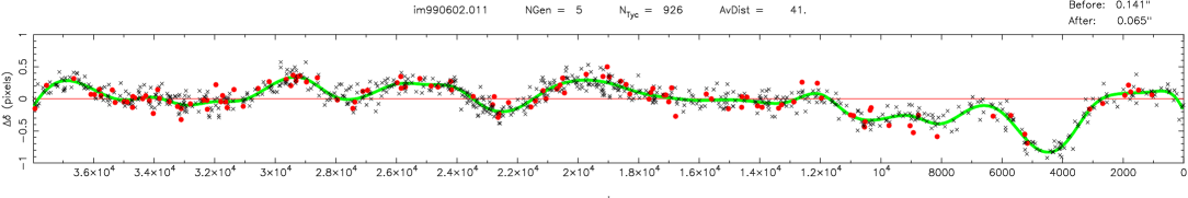
Figure 1: This shows an example of the Tycho 2 calibration functions for declination for a particular frame. The red points are the residuals from the primary frame. The crosses show the data from the overlapping frames. The green line is the derived final calibration function. The units of the residuals (CMT $-$ Tycho 2) are in pixels ($\sim$0.7^′′). In the calibration programme the RA values are normalized in order to improve the numerical stability of the solution. The actual range is 38,500 pixels and is the same as in Figure 2.

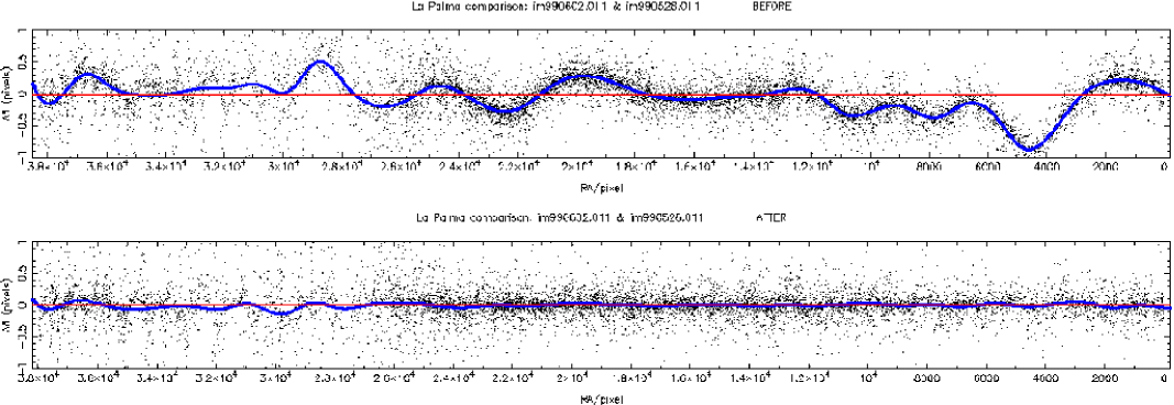
Figure 2: This shows an example of a night-to-night comparison for declination. The top plot is before the calibrations have been applied and the bottom one afterwards. Most of the fluctuations come from one night (2nd June 1999) as can be seen from the calibration plot (Figure 1). The reduced number of stars and increased number of outliers on the left of the plots is due to cloud coming over during the exposure. While this affects these plots, which mainly show the fainter stars, the calibration plots only contain bright stars ($r^{\prime}_{\rm CMT}<$12) and are thus not affected.

Observations of the survey are carried out on a declination grid of 15 arc minutes. Observations taken on different nights at adjacent declinations will have an overlap of about 36%. This is sufficient to define a transfer function (using all the stars in the frame) which characterizes the difference in the fluctuations between two nights. By applying these differences to the positions in the second frame the fluctuations of the secondary night are effectively transformed into those of the primary.

The transfer function is simply a set of cubic splines. The initial set of knots are placed at intervals of 1000 pixels ($\equiv$ 45 seconds of time). If a smaller interval was used, then the transfer function would map out a higher frequency than would be valid. This is determined by the highest frequency of fluctuations observed, which is in turn determined by the effective exposure time ($\equiv$ 2000 pixels $\equiv$ 90s). After the initial placement of knots has been made, the data is checked to see if there are enough points (10) present to define the splines reliably. If this is not the case, then the two knots in question are merged. This is carried out iteratively until the criterion is met for all knots.

The transformed positions from the secondary nights are then added to those from the primary night. Further frames that overlap this “new” extended frame are searched for and added in a similar way. This process can be carried on until there are a sufficient number of standards in the frame. However, the further away from the original data the transfer functions are calculated, the greater the problems arising from the propagation of errors from multiple application of transfer functions.

Investigations were carried out to determine the optimal number of generations to go from the original data. This was done using the residuals with respect to the Tycho 2 standards within the original frame. It was found that the best value varied between 4 and 9 generations, but the higher values tended to be less robust. A value of 5 generations was chosen as a reasonable compromise which produces consistently good results.

After building up a large frame, Tycho 2 stars are matched and the fluctuations mapped using a calibration function. In this case, the calibration function characterizes the difference between the primary night and the Tycho 2 positions. This is then applied to the positions of the primary night (only) to produce a calibrated output file. While transformed positions from the overlapping frames could be output at this point it is not done since their accuracy has been degraded via the night-to-night transfer functions. It is better to run the algorithm separately for each frame.

A similar procedure is carried out to calculate the calibration function to that used in determining the transfer function. A density of higher than 1 Tycho 2 star per 200 pixels is needed in order to obtain a reliable final calibration function.

Figure 1 shows an example of the final Tycho 2 calibration function for 5 generations of overlapping frames. This frame was chosen since it was from a particularly bad night and has very large fluctuations. Note that the rightmost trough of the declination plot does not have enough primary standards to define it adequately, but the addition of the standards from the overlapping frames provides enough information to calibrate the trough correctly.

After calibration, the residuals with respect to Tycho 2 are normally between 50 and 80 mas and mainly reflect errors in Tycho 2. Because of this, it is difficult to estimate the CMT external errors from these residuals.

After applying this calibration method to two overlapping frames a comparison was carried out. The results are shown in Figure 2. The two frames are from the nights of the 28th May and 2nd June of 1999. Most of the differences seen originate from the fluctuations on the 2nd June (see Figure 1). As can be seen in the AFTER plot, most of the fluctuations have been removed.

4.4 Other systematic effects

Each time the preliminary calibration programme is run, the residuals with respect to Tycho 2 in right ascension, declination and magnitude are accumulated. The systematics in this data are shown in Figure 3.

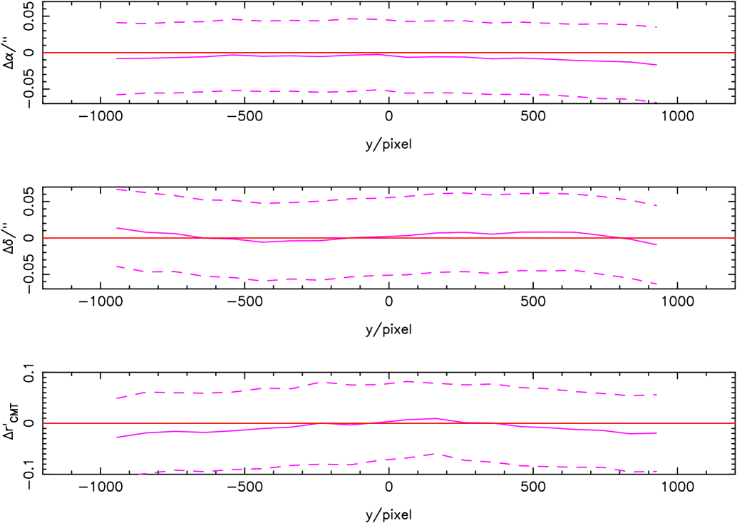
Figure 3: These plots show the accumulated residuals with respect to Tycho 2 as a function of $y$ ($\equiv$ declination) for stars brighter than $r^{\prime}_{\rm CMT}=10$. The solid line shows the median of the distribution and the dotted line the width.

Although these systematic errors are not very large in comparison with the random errors for bright objects, they should be corrected. Cubic polynomials were fitted to the data and applied in the calibration.

Investigations were carried out to see if the positional distortions were comparable with known effects. The effect of tangential projection can easily be estimated using a simplistic “$\tan\theta$” analysis. This is because drift scanning has smeared out most of the projection effects in right ascension and simplified the problem to a one-dimensional one. This will cause a distortion in declination of order of 3 mas. The systematic effect observed in declination is around 20 mas peak-to-peak.

As mentioned above, one of the effects of drift scanning is to smear out the projection effects (Gibson & Hickson (1992); Stone et al. (1996)). Using the equations below, taken from Taff (1981), the effect of image distortion can be calculated from projecting a spherical surface onto a flat plane (CCD chip).

$$\xi = {\cot\delta\sin(\alpha-\alpha^{*})}\over{\sin\delta^{*}+\cot\delta\cos\delta^{*}\cos(\alpha-\alpha^{*})}$$ (2)

$$\eta = {\cos\delta^{*}-\cot\delta\sin\delta^{*}\cos(\alpha-\alpha^{*})}\over{\sin\delta^{*}+\cot\delta\cos\delta^{*}\cos(\alpha-\alpha^{*})}$$ (3)

(For further detail regarding these equations see Taff (1981)).

Not only was the width of the image distortion investigated, but also the median position of the image. The width analysis produces results very similar to those of Figure 10 in Stone et al. (1996).

For the median of the positions, in right ascension, no systematic shift was observed since the effect of drift scanning is to distort the image symmetrically as long as the image is exposed equally either side of the meridian, ie. a complete drift scan over the CCD chip which is centred on the meridian. In declination, the situation is different in that the image is distorted towards the celestial pole. However, in order to affect the astrometry it is the difference in this distortion between the top and bottom of the CCD chip that is important. Results from the analysis showed that this effect is very small ($\sim$4 mas) and not greatly affected by the declination of the observation (for declinations less than $60^{\circ}$). Also, when a fit is carried out with respect to the Tycho 2 standards, the solution of the declination scale removes most of this systematic error.

The conclusion of this analysis is that projection effects and differential image distortion does not account for the systematic effects observed in right ascension and declination.

The systematic effect in magnitude as a function of $y$ (equivalent to declination) is discussed in Appendix B.

A small systematic effect also exists in declination as a function of colour. This is caused by the wavelength dependence of atmospheric refraction. Using a spectral atlas it is possible to calculate the correction appropriate for the passband defined by the $r^{\prime}$ filter and the response of the KAF-4202 CCD chip. This method is outlined in Evans & Irwin (1995), except that for the calculations in this paper the data from Pickles (1998) was used rather than from Gunn & Stryker (1983) and an average atmospheric pressure of 780 mbar was used.

These corrections are within 1 or 2 mas to those given in Table 2 of Stone (1997) after accounting for the difference in atmospheric pressure. However, there is a larger difference for the reddest stars (B$-$V$>$1.4). This is possibly due to detailed differences in the passbands of filters used at the two telescopes. The correction that should be applied to the data, $\Delta R$, can be calculated from Equation 4. This relation is also shown in Figure 4, which shows the detailed results from the spectral flux analysis. From this diagram can also be seen that for the reddest stars the relation deviates from linear and might provide another reason for the slight difference with the results in Stone (1997).

$$\Delta R=-13.5[{\rm(B-V)_{J}}-0.60]\enskip({\rm mas})$$ (4)

Although the analysis calculates an absolute constant of refraction, it is only a relative term that is required as a correction since the calibration with respect to Tycho 2 has already accounted for the average refraction term. In the above equation, the offset used is the average colour of the Tycho 2 stars used in the calibrations. This was found to be $\rm(B-V)_{J}=0.60$ (equivalent to $\rm(B-V)_{T}=0.71$, see Equation 1.3.20 of Volume 1 of ESA (1997)). This colour corresponds to that of a G0 star.

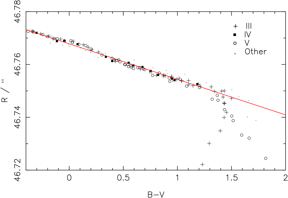
Figure 4: This plot shows the constant of refraction as a function of (B$-$V)_J. The various symbols stand for different types of star. The line drawn is the best fit line to the points with (B$-$V$)_{\rm J}<$1.2 and is equivalent to that given in Equation 4.

This correction can then be applied to the declination using the following formula:

$$\delta_{\rm corr}=\delta+\Delta R\tan z/3.6\times 10^{6}\enskip({\rm degrees}),$$ (5)

where $\Delta R$ comes from Equation 4 and $z$ is the zenith distance, with this being positive for stars North of the zenith. Since colours are generally not available for the stars in the survey, this correction has not been applied, however for the majority of stars in the survey ($\rm 0.0\lesssim(B-V)_{J}\lesssim 1.5$), $\Delta R$ varies by about $\pm 10$ mas and consequently the correction to declination will be less than 10 mas for all the survey cf. the astrometric accuracy for the bright end of 36 mas.

5 Photometric data reductions

The main part of the photometric reductions are carried out by the same calibration programme described in Section 4.2. The photometric data used as the standards are the $B_{T}$ and $V_{T}$ values from the Tycho 2 catalogue. Although there are catalogues with higher accuracies at the faint end, Tycho 2 is uniquely homogeneous and dense. However, not all Tycho 2 stars were used. In order to make the photometric reductions more robust, stars identified as variable were excluded from the calibration. Due to the nature of the reduction process used to create Tycho 2, variability information is not available in that catalogue. For this, the original Tycho data (ESA (1997)) must be used.

The intensities determined from the images (see Section 4.1) are first converted into magnitudes ($m=-2.5\log_{10}i$) and are then corrected in order to take into account the difference between isophotal and total magnitudes (see Section 5.1). Following this, the calibration then simply consists of determining the zero point of the magnitude scale.

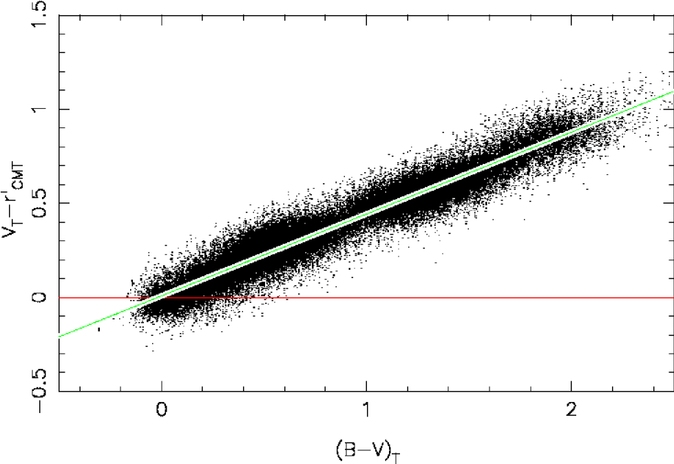
Figure 5: This colour-colour diagram shows the relationship between the Tycho 2 magnitudes and the CMT instrumental magnitude, $r^{\prime}_{\rm CMT}$. Only stars brighter than $\rm V_{T}<10$ were used in the determination. The green line is a least-squares linear fit to the data.

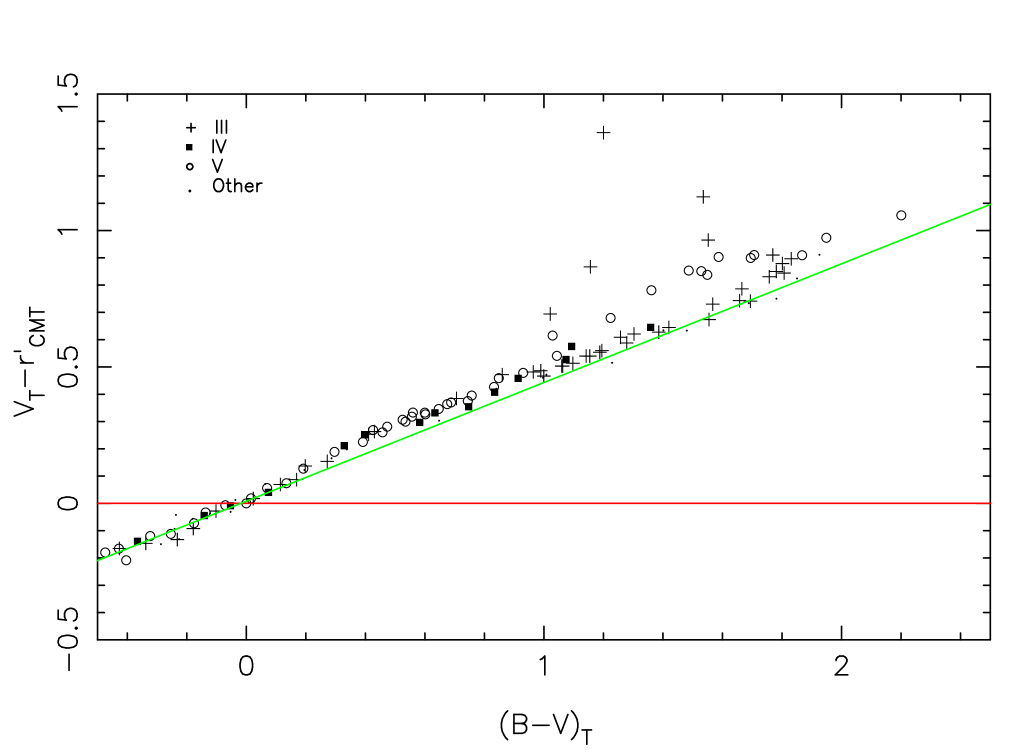
Figure 6: The results of synthetic colour calculations are shown in this plot. The various symbols stand for different types of star. The line drawn is the same as that in Figure 5.

Since the CMT only observes in one passband, photometry from the telescope cannot be placed on a standard photometric system without additional colour information. However, using the colour data in the Tycho 2 catalogue, it is possible to calibrate onto the instrumental magnitude system. Figure 5 shows the least-squares solution used to determine the linear colour term. This was found to be $\rm 0.435\times(B-V)_{T}$.

By using this a priori colour term, the $V_{T}$ of the Tycho 2 standards can be converted into the natural system of the CCD and filter combination. This is close to the Sloan $r^{\prime}$ passband, but will be on the Vega scale rather than the spectrophotometric AB_ν magnitude system (Fukugita et al. (1996)).

To test that this colour term was reasonable, synthetic colours were generated in a manner similar to that in Evans (1989). Again, the difference being the use of data from Pickles (1998) rather than from Gunn & Stryker (1983). The resulting colour-colour diagram is shown in Figure 6 along with a line representing the colour term that was determined from the CMT data. At the red end, the line lies close to the giant stars rather than the main sequence stars. This agrees with the expectation that for V$<$10, almost all red stars are giants (Besançon Galaxy Model, Robin & Crézé (1986)).

When determining the zero point, a weighted least-squares solution is used along with a rejection filter to identify outliers. A number of diagnostics are determined in this solution. The main ones are the scatter of the residuals from the calibration and the magnitude limit. The former gives an indication of the quality of the photometric conditions, while the latter will show the presence of cloud. In addition to this, a median filter is applied to the photometric residuals as a function of time in order to determine if an exposure was interrupted by cloud. Depending on the level of the cloud opacity, parts of a data frame can be flagged as non-photometric or not suitable for the survey. In the latter case, this is when the effective magnitude limit of a part of an exposure is brighter than $r^{\prime}_{\rm CMT}=16$. This information is then passed to the selection programme so that another observation can be rescheduled. Non-photometric observations are accepted into the survey, since the primary purpose of the survey is astrometry.

5.1 Linearized photometry scale

Checks have been carried out using timed exposures to confirm the linearity of the CCD. These show that the CCD is linear to at least the 1% level all the way up to when the CCD saturates at about 60,000 counts. This corresponds to an $r^{\prime}_{\rm CMT}$ magnitude of 8–9 for typical observing conditions.

Since the photometry is derived from isophotal intensities a correction is required to obtain total magnitudes. Since the image profiles have been found to be exponential, the appropriate correction from Irwin & Hall (1983) has been applied. Investigations into an alternative method of linearizing the photometry scale using a variant of the algorithm developed by Bunclark & Irwin (1983) have also been carried out.

5.2 Photometric extinction

With the photoelectric micrometer, the photometric solution that was carried out each night followed a more classical solution (Carlsberg Consortium (1999)), with the extinction in V being calculated as part of the photometric solution. This data was published regularly on the Internet and covered the years 1984–1998.

From June 1998, since a CCD was being used, the observing strategy and the part of the sky being observed, prevented a classical solution of the extinction being made since there was not a large enough range in $\sec z$. However, by assuming that the zero point of the photometric solution only changes gradually over time and that the lowest measurable extinction would correspond to the dust-free value for $r^{\prime}_{\rm CMT}$ (0.09), it is possible to derive an extinction value for each relatively stable night.

To do this, the zero point determined from the photometry is first corrected for exposure time ($\equiv\cos\delta$) and then a simple linear model is applied to account for the change in sensitivity of the system. Finally, a correction for $\sec z$ is applied in order to produce an extinction value. Although this is only for the $r^{\prime}_{\rm CMT}$ passband, it is possible to generate extinction values for other passbands using the data contained in King (1985).

Since March 1999, extinction values for $r^{\prime}_{\rm CMT}$ have been published on the Internet, cf. the earlier data. In these tables the mean for each night is given using only those CCD frames that were considered photometric. On average, each data frame has 30–40 calibrating stars in it.

Even though this is not a customized extinction monitor, such as Hogg et al. (2001), the CMT extinction data is currently the only source of regular extinction measurement available on the La Palma site and thus provides a valuable service.

6 Error estimation

In order to measure the internal errors of the catalogue, data can be used from the overlap regions and repeat observations. The results of such an analysis are given in Table 2. However, it must be understood that since correlations exist between the data and unaccounted for systematic errors, these measurements will tend to underestimate the true, external, errors of the data.

Table 2: The median internal and external errors for the CMT. The units for the RA and declination are milli arc seconds and those for the magnitudes are millimagnitudes.

Internal
$r^{\prime}_{\rm CMT}$	RA	Dec	Mag
$<$13	21	21	16
14	31	26	30
15	55	42	58
16	112	91	124

External
$r^{\prime}_{\rm CMT}$	RA	Dec	Mag
$<$13	36	37	25
14	45	40	35
15	68	55	70
16	113	90	170

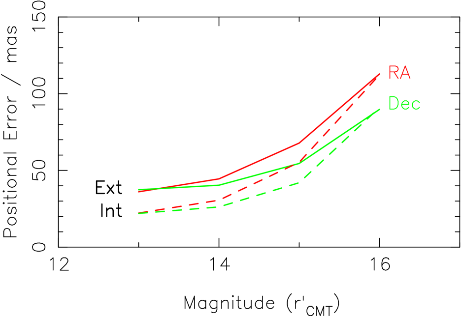
Figure 7: The internal and external positional errors as a function of magnitude. The solid line gives the median external errors and the dashed line shows the equivalent internal errors. RA is shown in red and declination in green.

The measurement of external errors can be problematical since it requires a comparison with another catalogue where the errors are either much smaller, and the residuals yield the external errors directly, or where the errors are very well determined, and can thus be accounted for in the residuals. In the former case, not many such catalogues exist and even in those cases the data is quite sparse, and in the latter, the estimation is dependant on the external errors of the comparison catalogue being reliable.

A comparison of the CMT data has been carried out with respect to Tycho 2, but this did not yield very useful results since it was limited to the brighter end ($r\,^{\prime}_{\rm CMT}<12$) of the CMT catalogue. Also, the average error of a faint Tycho 2 star, which is in common with the CMT data, is slightly larger than the average CMT error. In combination with the low number of stars in these comparisons, this makes a CMT error calculation difficult to estimate using just Tycho 2 data. Although the results are quite noisy, it is possible to produce an approximate external error for the CMT catalogue of 40 mas.

Another technique available involves the use of 2 or more deep comparison catalogues, where it is then possible to measure the external errors directly of all the catalogues involved without having to assume any external error measurements. As with a comparison with a single catalogue, allowance must be made for proper motions and, if the epoch difference between the catalogues is large, the errors in the proper motions.

The basis of the technique is the assumption that the residuals between any two catalogues result from the quadrature sum of the external errors. If three catalogues exist, it is possible to derive these external errors from the three sets of residuals by simple substitution. If an appreciable epoch difference exists, an allowance must be made for the errors in the proper motions used in the comparison. This acts as an additional term in the quadrature sum and has to be removed using the quoted proper motion error values.

Comparisons with the FASTT and UCAC catalogues (Stone et al. (1999), Zacharias et al. (2000)) using this technique showed that the astrometric accuracy of the CMT catalogues, before secondary calibrations (atmospheric fluctuations and CTE correction) are carried out is 50–80 milli arc seconds (mas) at the bright end. After such calibrations are applied, the accuracy improves to 25–45 mas. The dependency of these accuracies as a function of magnitude is given in Table 2. Although only one value is quoted per magnitude bin in these tables, there exists a range of accuracies, as quoted earlier, which is caused by the varying density of Tycho 2 standards across the sky. For a region of the sky which has more standards in it, the accuracy of the catalogue at that point will be better.

Figure 7 shows these results in graphical form. For bright stars ($r\,^{\prime}_{\rm CMT}<13$), the accuracy of the astrometry is about 35 mas for both RA and declination, but as you go fainter the accuracy in RA becomes gradually worse than that for declination. The most probable explanation is that this is caused by further effects resulting from the CTE problem which the calibration has not yet accounted for. This would only affect RA.

For photometry, the external accuracy estimates are more uncertain since the comparison catalogues are not primarily photometric ones. Additionally, there are probably some differences in the passbands used, which would result in unaccounted colour terms. Assuming the quoted errors from Stone et al. (1999), a comparison with the FASTT data yields rough estimates for the external errors and are given in the external part of Table 2. The internal photometric errors were calculated from the overlaps in the same way as that for the astrometry and are also given in this table.

7 Description of the released catalogue

After the fluctuation calibration has been carried out, the data frames undergo a further 6-parameter linear fit (see Equation 1) using the Tycho 2 standards. This is done since the residuals have been reduced and a more accurate fit can be achieved.

The final catalogue consists of the averaged positions from the calibrated data frames. For the current version only a simple algorithm is used whereby any images within $2^{\prime\prime}$ of each other are considered as the same source. However, considering that the average image size is larger than this, it is likely that this algorithm is sufficient.

The current release of the catalogue (Version 1.0) covers the declination zone $-3^{\circ}<\delta<+3^{\circ}$. The data is available over the Internet where the format of the catalogue is described. The main part of the survey extends to $+30^{\circ}$ and further releases of the catalogue which will complete the coverage will be available in the future from the same location. An extension of the survey is planned, extending it to $+50^{\circ}$ in the North and $-15^{\circ}$ in the South.

8 Conclusions

By upgrading the Carlsberg Meridian Telescope to have a CCD operating in drift-scan mode, a new lease of life has been breathed into the telescope. It should be pointed out that this will only be useful over the next ten years or so. Then, data from astrometric satellites such as DIVA and GAIA will become generally available and supersede the astrometric accuracy of what can be achieved from the ground. It is thus important that planned upgrades of meridian telescopes are carried out as soon as possible and that the results are published promptly so that the maximum use can be made of the data.

The results shown here demonstrate that using transfer functions it is possible to calibrate the fluctuations caused by atmospheric turbulence using just the Tycho 2 stars. This is a more efficient method than using a subcatalogue since multiple measurements of the sky are not required.

After this calibration, the external accuracy achieved for the brightest stars in the survey is 36 mas in right ascension and declination and 0.025 magnitudes in $r^{\prime}_{\rm CMT}$ photometry.

The web site of the telescope is at:
http://www.ast.cam.ac.uk/~dwe/SRF/camc.html

Appendix A Calibration of CTE feature

Initial comparisons carried out with respect to astrometric standards published by Stone and co-workers (Stone (1997); Stone et al. (1999)) indicated that a large systematic difference in right ascension existed.

Investigation of the raw data showed that no large image asymmetry was present. Further comparisons made with data released from Bordeaux confirmed that the systematic difference was a feature of the CMT data.

It was soon established that this effect was caused by problems with the charge transfer efficiency of the CCD. Detailed investigations of the CTE properties of similar CCD chips were carried out by Copenhagen University Observatory (Sørensen et al. (2000)). Contact with other groups revealed that this wasn’t an isolated case (Zacharias et al. (2000)). Various solutions are available to reduce the magnitude of this effect which include fine tuning the electronics and increasing the temperature of the CCD. However, there is still a need to calibrate this effect since the data originally taken, before the final set-up was in place, could still be used and also the effect isn’t fully removed by these changes.

The observed effect of this problem is to cause a systematic shift in RA as a function of magnitude (see Figure 8). On top of this, the effect is also a function of the background illumination which reduces the effect the brighter the sky. This is similar to the reasons needed for a preflash with early CCDs which also had CTE problems. A continuous illumination system was considered for the camera to increase the background level and reduce the effect. However, time and resources were not available to carry out this experiment.

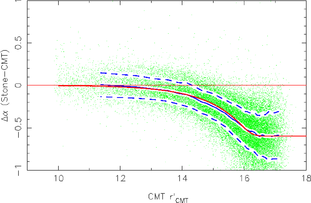
Figure 8: This plot shows the general trend in RA caused by the charge transfer efficiency problem. This is a comparison, using observations taken during dark conditions, with respect to Stone’s standards. A three-parameter model has been fitted to the data.

Initial work compared data from the Stone standard regions and fitted a 3-parameter function,

$$\Delta\alpha=max(-\exp(ax+b),c),$$ (6)

where $x$ is the magnitude, for various ranges of background value. A problem with this function was that no trend could be seen in the parameters ($a,b,c$) as a function of background and thus further examination of the effect would not be possible.

Additionally, the CTE characteristics changed on 9 August 1999, thus a new calibration would be needed. This was indicative of a progressive failure of the camera controller circuitry. It failed totally at the beginning of October 1999 and had to be replaced.

Since the equator had already been covered by the survey, it was unclear whether we had enough data, for all periods, to calibrate the problem properly. Although brief comparisons had also been carried out with respect to other telescopes (Bordeaux), there was insufficient data to provide a calibration. It was thus desirable to compare with other data sets.

Period	Start	End	Controller	Temperature	Number of	%
					observations
					(1000’s)
0	990331	990408	1	$-65\degr$C	518	1
1	990409	990806	1	$-58\degr$C	10,721	23
2.1	990809	990821	1	$-58\degr$C	976	2
2.2	990823	990923	1	$-58\degr$C	1,630	3.5
2.3	990924	991007	1	$-58\degr$C	1,199	2.5
3	991101	991213	2	$-65\degr$C	1,042	2
4	991214	000127	2	$-54\degr$C	1,741	4
5	000128	000930	2	$-30\degr$C	28,626	62

Table 3: This table shows the different calibration periods identified along with some of the characteristics of the periods. The data analysed only covers up to the end of September 2000.

Palomar Observatory Sky Survey II (POSS2) data was obtained for 27 fields. These had been scanned by the APM (Kibblewhite et al. (1984)). This data was matched with the CMT CCD data and the residuals plotted as a function of magnitude (cf. Figure 1) for various sky brightness ranges. Although this data was less accurate than that of Stone, more data was available.

Initially, the data was split into 5 periods (1–5), depending on which CCD controller was in operation and what the CCD temperature was. The Controller 1 period was split into two due to the change in CTE characteristics mentioned above.

While carrying out the overlap analysis (see later) it was realized that the first data period had different characteristics, so was split into Periods 0 and 1. This corresponds to a change in the CCD temperature caused by vacuum problems within the camera. Also, the calibration was very unstable for Period 2, so it was split into three. Table 3 shows the different calibration periods finally adopted.

In analysing this data, it became clear that the ($a,b,c$) model was not good enough. The replacement model eventually chosen was a simple scaled model. In this model the functionality with magnitude was taken directly from the darkest sky bin of the POSS2 data comparison (the one with the largest effect) and then scaled to fit the other sky brightness bins. Thus the parameterization had been reduced from 3 to 1, the scale value, which could then, in turn, be plotted as a function of sky brightness to see if further parameterization could be carried out. The scale value was defined to be equivalent to the RA shift at the faint end (in arc seconds).

The results of these calibrations are shown in Figure 9. A simple exponential has been fitted to the data:

$$scale=z\exp(-sky/y)$$ (7)

with the data split into four periods: 0/1, 2.*, 3/4 and 5. $y$ and $z$ in this equation are the free parameters of the fit.

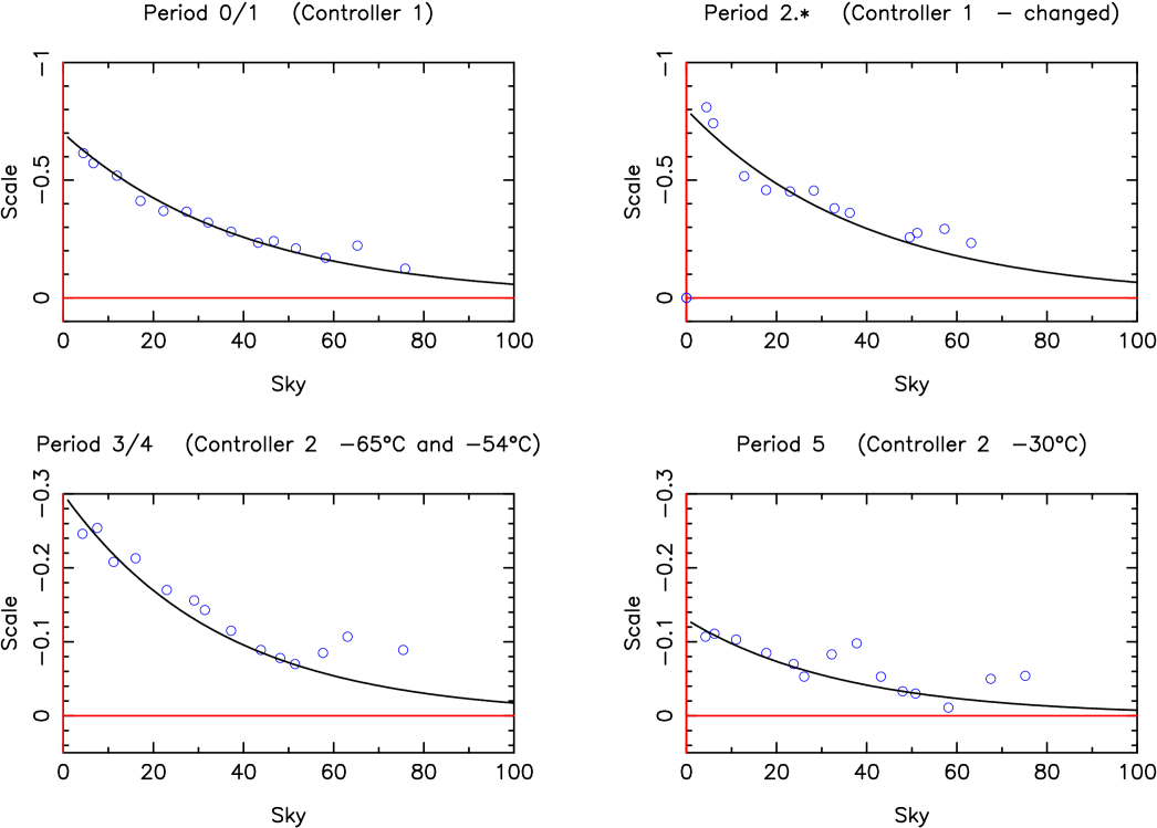
Figure 9: This plot shows the scale value plotted versus sky brightness for 4 different periods. A simple exponential has been fitted to the data.

These diagrams demonstrate that a simple parameterization exists for the CTE calibration covering the entire survey. They also clearly show the effect of the various changes made to the CCD camera. At the start of the project the maximum size of the CTE shift ($z$) was about $0.7^{\prime\prime}$. The new controller reduced this down to $0.3^{\prime\prime}$ due to improved voltage settings and finally the increase of the CCD temperature from $-65\degr$C to $-30\degr$C reduced it further to $\sim 0.1^{\prime\prime}$.

Work on the UCAC comparisons lead to the implementation of a CTE “problem spotter” in the catalogue generation programme via the overlaps. If any of the overlap comparisons show an RA trend after the CTE calibrations have been carried out, it indicates a problem in one (or both) of the two frames of the overlap. Many overlap pairs in the survey were flagged as having problems, thus indicating that a four-period scaled model, characterized by Figure 9, was too simplistic.

An analysis was then carried out on all the residual CTE shifts. Firstly, all overlaps were determined (14,000 overlaps for 5,600 frames) and the relative CTE shift for each overlap calculated. At this point we only have information on the overlaps and do not know the individual contribution from each frame. Then, for each frame, the median CTE shift for all its overlaps is calculated, taking care with the signs of these overlap shifts. If most of the calibrations for the frames are correct, then the median will give a good approximation to the CTE shift remaining for that frame. We can then use these frame values to correct the overlap values and then improve our original estimates of the frame values by iteration. This process converges after about 5 iterations.

Note that this is all carried out after a standard CTE calibration had been applied. Thus, the presence of outliers or increased scatter in the results indicates a problem with the current calibration.

Figure 10 shows the residual CTE shifts for each frame as a function of time. Using a figure like this, it was possible to subdivide the original 4 periods, as used for Figure 9, into the periods indicated in Table 3. For each period, by plotting the residual against sky background you can improve the CTE calibration for that period. In addition to using an exponential model, for some periods, it was necessary to use a model of the form $scale=a/(b+sky)$, cf. Equation 7.

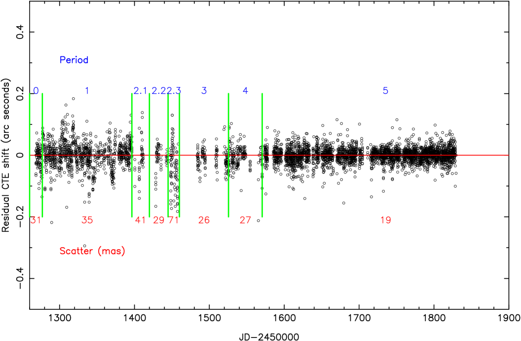
Figure 10: This plot shows the residual CTE shift (after calibration) as a function of time.

Also shown in Figure 10 is the scatter for each period. This gives an indication as to how well the calibration has been carried out. The improvement in the calibration as the survey has progressed simply reflects the reduction in the overall level of the CTE problem.

Period 2 has a high scatter because it generally contains poor data. Originally, data from this period had a much higher scatter. Closer analysis showed that a large part of this came from a few nights. Thus, it was decided to delete 4 nights (5, 6, 15 and 18 September 1999) from the survey. Doing this loses about 650,000 observations (about 1% of the data so far).

From the scatters shown, it can be seen that the CTE problem has been solved to about the 100 mas level for the faint end (3 sigma limits), cf. the faint end random errors of approximately 100 mas. Figure 8 can be used to gauge how this number translates to brighter magnitudes.

Appendix B Flat-fielding

No multiplicative flat field is applied to the raw frame data in the image analysis because of the difficulty in separating multiplicative (flat field) and additive (bias) components and because of the small size (1%) of the effect (see Figure 11). Additive (bias and sky) corrections are carried out and the image analysis programme removes the bias as a one-dimensional function in $y$, combined with a one-dimensional function in $x$ to remove background variations.

Although the raw image data is not kept, the flat-field information is archived every night. Since the CCD camera takes drift-scan observations, the flat fields are one dimensional. Not all the frames will have a flat field since if the sky level is too low then no reliable flat field can be calculated. About two thirds of the frames do not have any flat-field information.

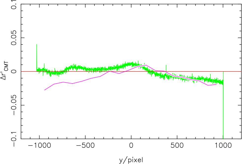
Figure 11: This plot shows a typical flat field for high sky brightness conditions (noisy solid line). Also shown is the systematic effect in magnitude from Figure 3 (solid line).

Figure 11 shows a typical flat field from a frame with a high sky level. Monitoring of the flat fields shows that the main variation seems to be as a function of sky level. If the sky level is high, then the flat field is fairly flat ($\pm$1% level). If the sky level is low, then there is about a 10% variation at one edge of the CCD, most likely caused by just a change in the y-dependent bias level. Over time there is hardly any change in the general flat field shape, however, occasionally a flat field shows a significant difference of a few percent over the 2000 pixels. Closer investigation has shown that these changes are caused by changes in the background and not the sensitivity of the CCD.

Various investigations were carried out to determine whether the measured flat fields represent a multiplicative correction or not due to the problem of disentangling bias and sky.

One experiment was to apply the flat fields during the initial calibration after the preliminary data reduction. Normally, each column would be scaled by the corresponding one in the flat field. For this test, the appropriate column used was the average $y$ value of an image and the corresponding scaling factor was applied to the whole image. Since this was already an approximation, a median filter was applied to the flat field data in order to reduce the level of noise.

After re-reducing the data, a comparison was made with respect to Tycho 2 This showed that the flat fields were not appropriate to use since extra systematic effects at the level of $\sim$5% were now visible. This implies that what is measured as the flat field has at least an additive component, as pointed out above.

As mentioned before, gradients are seen in some of the flat field comparisons. These are of order a few percent over the width of the CCD chip. These tend to happen during periods of bad weather, possibly indicating partially illuminated cloud causing a real gradient in the background and hence an additive effect.

To check this, a comparison was carried out on one particular frame, which has a 5% variation, and a number of overlapping frames. No variation could be seen in the photometry as a function of $y$ for $r^{\prime}_{\rm CMT}<14$. This indicated that the sensitivity was not varying across the chip. A variation is seen for a sample of faint images. This is consistent with background levels varying with $y$ causing problems with the isophotal correction.

Also shown in Figure 11 is the magnitude systematic from Figure 3. The obvious feature of this plot is that one side matches up reasonably well, while the other doesn’t.

Considering the significant differences between the measured flat fields and the photometric corrections derived from the external standards, it was decided that there was no point in using the flat field information in the photometric calibration.