The Three-Point Correlation Function in Cosmology

Abstract

With the advent of high-quality surveys in cosmology the full three-point correlation function will be a valuable statistic for describing structure formation models. It contains information on cosmological parameters and detailed halo properties that cannot be extracted from the two-point correlation function. We use the halo clustering model to analytically calculate the three-point correlation function (3PCF) for general cosmological fields. We present detailed results for the configuration dependence of the 3-dimensional mass and galaxy distributions and the 2-dimensional cosmic shear field. We work in real space, where higher order correlation functions on small scales are easier to measure and interpret, but halo model calculations get rapidly intractable. Hence we develop techniques that allow for the accurate evaluation of all the contributing terms to real space correlations. We apply them to the 3PCF to show how its configuration and scale dependence changes as one transits from the nonlinear to the quasilinear regime, and how this depends on the relative contributions from the 1-, 2- and 3-halo terms.

The 3PCF violates the hierarchical ansatz in both its scale and configuration dependence. We study the behavior of the coefficient $Q$ in the expansion: $\zeta(r_{12},r_{23},r_{31})=Q[\xi(r_{12})\xi(r_{23})+\xi(r_{12})\xi(r_{31})+\xi(r_{23})\xi(r_{31})]$ from large, quasilinear scales down to about 20 kpc. We find that the nonlinear 3PCF is sensitive to the halo profile of massive halos, especially its inner slope. We model the distribution of galaxies in halos and show that the 3PCF of red galaxies has a weaker configuration and scale dependence than the mass, while for blue galaxies it is very sensitive to the parameters of the galaxy formation model. The 3PCF from weak lensing on the other hand shows different scalings due to projection effects and a sensitivity to cosmological parameters. We discuss how our results can be applied to various analytical calculations: covariances of two-point correlation function, the pairwise peculiar velocity dispersion, higher-order shear correlations, and to extend the halo model by including the effects of halo triaxiality and substructure on statistical measures.

1 Introduction

Understanding the nature of the large-scale structure and the evolutionary history of the universe is the central aim of cosmology. Therefore, quantifying the observed distribution of matter rigorously is of fundamental importance, and $n$-point correlation functions have been the most widely used statistical tools for this purpose (e.g., see Peebles 1980). The inflationary scenario predicts Gaussian initial conditions. The statistical properties of the Gaussian field are fully characterized by the two-point correlation function (2PCF) or its Fourier transform, the power spectrum. Based on this idea, the two-point statistical measures for various cosmological fields have been extensively used for testing the paradigm as well as constraining cosmological parameters; the galaxy distribution in the redshift catalog (e.g., Totsuji & Kihara 1969; Hamilton & Tegmark 2002), the cosmic microwave background anisotropy (e.g., de Bernardis 2000) and the cosmic shear field (e.g., Van Waerbeke et al. 2001). However, even for Gaussian initial conditions, nonlinear gravitational instability induces non-Gaussian signatures in the mass distribution, which contain information on the nature of gravity and the dark matter. The three-point correlation function (3PCF), or equivalently, its Fourier-transformed counterpart, the bispectrum, is the lowest order statistical tool to probe the non-Gaussianity. The 3PCF can place strong constraints on models of structure formation. As an example, the measurements of the bispectrum in the galaxy distribution at the large scales ($\lower 2.15277pt\hbox{$\;\buildrel>\over{\sim}\;$}10~{}h^{-1}{\rm Mpc}$) have been used to determine the bias parameter as well as to constrain the primordial non-Gaussianity (e.g., Feldmann et al. 2001; Verde et al. 2001). It is also expected that the 3PCF of the cosmic shear field can be used to precisely determine the cosmological parameters complementary to the measurements of the 2PCF (e.g., Bernardeau, Mellier & Van Waerbeke 2002; Bernardeau, Van Waerbeke, & Mellier 2003).

In this paper, we focus on developing a theoretical model of the 3PCF in real space for 3D and 2D cosmological fields. In practice, on small scales the 3PCF would be easier to measure from observational data over the bispectrum, since it does not require the Fourier transform for the survey data that usually have a complicated geometry of data fields.

Theoretical models of the weakly nonlinear 3PCF have been well studied in the literature based on perturbation theory [Fry 1984b, Jing & Börner 1997, Gazta$\tilde{\rm n}$aga & Bernardeau 1998, Frieman & Gaztañaga 1999, Barriga & Gaztañaga 2002]. Perturbation theory can describe properties of the dark matter and galaxy clustering on large scales $\lower 2.15277pt\hbox{$\;\buildrel>\over{\sim}\;$}10~{}h^{-1}{\rm Mpc}$ and predict that the 3PCF depends on the shape of triangle configuration and, as a result, contains information of the primordial power spectrum and the galaxy biasing. Historically, the pioneering measurement of the galaxy 3PCF done by Peebles & Groth (1975) (also Groth & Peebles 1977) proposed the “hierarchical form”, $\zeta(r_{12},r_{23},r_{31})=Q[\xi(r_{12})\xi(r_{23})+\xi(r_{23})\xi(r_{31})+\xi(r_{31})\xi(r_{12})],$ with the constant $Q\simeq 1.3$. However, subsequent work has revealed that the measured 3PCF does not obey the hierarchical form rigorously and the large-scale amplitudes can be explained by the perturbation theory results of the cold dark matter (CDM) models, if the biasing relation is correctly taken into account for the analysis [Jing & Börner 1998, Frieman & Gaztañaga 1999].

On the other hand, a quantitative theoretical model of the 3PCF in the strongly nonlinear regime is still lacking except for studies relying on $N$-body simulations (Matsubara & Suto 1994; Suto & Matsubara 1994; Jing & Börner 1998) . Simulations provide only limited physical insight into the complex non-linear phenomena involved in gravitational clustering, and are intractable for performing multiple evaluations in parameter space.

Therefore, the main purpose of this paper is to develop an analytical model for predicting the 3PCF applicable to both the linear and nonlinear regimes. For this purpose, we need a model to correctly describe the redshift evolution and statistical properties of gravitational clustering up to the three-point level. We employ the so-called dark matter halo model, where gravitational clustering is described in terms of correlations between and within dark matter halos. Originally, this model was developed to express nonlinear clustering as the real-space convolution of halo density profiles (Neymann & Scott 1952; Peebles 1974; McClelland & Silk 1977; and also see Scherrer & Bertschinger 1991; Sheth & Jain 1997; Yano & Gouda 1999; Ma & Fry 2000b,c). Most recent works have relied on the the Fourier-space formulation, since the forms of the power spectrum and the bispectrum become much simpler (Seljak 2000; Ma & Fry 2000c; Peacock & Smith 2000; Scoccimarro et al. 2001; Cooray & Hu 2001a,b; Berlind & Weinberg 2002; Hamana, Yoshida & Suto 2002; Takada & Jain 2002 hereafter TJ02; Scranton 2002; and also Cooray & Sheth 2002 for a recent review). The halo model appears remarkably successful in that, even though it relies on rather simplified assumptions, it has reproduced results from numerical simulations (Seljak 2000; Ma & Fry 2000c; Scoccimarro et al. 2001; TJ02) and also allowed for interpretations of observational results of galaxy clustering [Seljak 2000, Scoccimarro et al. 2001].

We formulate the 3PCF model so that it can be applied to general 3D and 2D cosmological fields, such as the mass and galaxy distributions and the cosmic shear fields. Our method is built on the real-space formulation for the correlations of three particles in one halo. This is because the real-space approach enables us to compute the one-halo contribution to the 3PCF by a 4-dimensional integration, which is an advantage compared to the Fourier space approach. For the 2- and 3-halo terms, we rely on the Fourier-space approach and the approximations presented in Scoccimarro et al. (2001; also see TJ02). We study the transition from the quasi-linear to nonlinear regimes and the relative contribution of the different terms to the 3PCF. We show the halo model predictions for the 3PCF of the mass and galaxy distribution and the weak lensing convergence field for the currently favored CDM model. To do this, we will focus on the dependences of the 3PCF on the triangle configurations as well as on the properties of the halo profile, its inner slope and concentration.

This paper is organized as follows. In §2 we present the formalism to compute the 3PCF of the 3D density field based on the real-space halo model and review the Fourier-space halo approach and halo model ingredients (halo density profile, mass function and bias model) we will use in this paper. In §3, we present the method to compute the angular 3PCF. In §4 we show the results of the halo model predictions for the 3PCF of the mass and galaxy distributions and the weak lensing convergence field. Finally, §5 is devoted to a summary and discussion. We give some useful approximations for calculating the 3PCF in Appendix A and B. We use the currently favored CDM model ($\Lambda$CDM) with $\Omega_{m0}=0.3$, $\Omega_{\lambda 0}=0.7$, $h=0.7$ and $\sigma_{8}=0.9$. Here $\Omega_{\rm m0}$ and $\Omega_{\lambda 0}$ are the present-day density parameters of matter and cosmological constant, $h$ is the Hubble parameter, and $\sigma_{8}$ is the rms mass fluctuation in a sphere of $8h^{-1}$Mpc radius. The choice of $\sigma_{8}$ for this model is motivated by the cluster abundance analysis [Eke, Cole & Frenk 1996].

2 Dark Matter Halo Approach

2.1 Real-space halo approach

In this section, we briefly review the real-space dark matter halo approach (McClelland & Silk 1977; Scherrer & Bertschinger 1991; Sheth & Jain 1997; Yano & Gouda 1999; Ma & Fry 2000b,c), where the $n$-point correlation functions are described by the real-space convolution of halo density profiles.

In the halo approach, we assume that all the matter is in halos with the density profile $\rho_{h}(\mbox{{\it\boldmath$x$}};m)$ parameterized by a mass $m$. The halo mass is given by

$$m\equiv\int_{V_{\rm vir}}\!\!d^{3}\mbox{{\it\boldmath$x$}}~{}\rho_{h}(\mbox{{\it\boldmath$x$}};m),$$ (1)

where $V_{\rm vir}$ is the virial volume of the halo. It is convenient to introduce the normalized halo profile defined as $u_{m}(\mbox{{\it\boldmath$x$}};m)=\rho_{h}(\mbox{{\it\boldmath$x$}};m)/m$, satisfying the condition

$$\int_{V_{\rm vir}}\!\!d^{3}\mbox{{\it\boldmath$x$}}~{}u_{m}(\mbox{{\it\boldmath$x$}};m)=1.$$ (2)

In this paper we employ the virial volume as the boundary of a given halo, which can be formally defined, for example, based on the spherical top-hat collapse model. However, since in reality some matter is distributed outside the virial region, it is non-trivial to choose which boundary condition to use for the halo model. We will discuss how this uncertainty affects the halo model predictions, and show that it does not matter in the non-linear regime.

The density field at some point can be given by the superposition of each halo density profile: $\rho(\mbox{{\it\boldmath$x$}})=\sum_{i}m_{i}u_{m_{i}}(\mbox{{\it\boldmath$x$}};m_{i})$. The mean density of the universe is thus obtained from the ensemble average (Scherrer & Bertschinger 1991)

$$\bar{\rho}_{0} = \langle{\rho(\mbox{{\it\boldmath$x$}})}\rangle=\left\langle{\sum_{i}m_{i}u(\mbox{{\it\boldmath$x$}}_{i}-\mbox{{\it\boldmath$x$}};m_{i})}\right\rangle=\int\!\!dm~{}mn(m)\int\!\!d^{3}\mbox{{\it\boldmath$x$}}^{\prime}u_{m}(\mbox{{\it\boldmath$x$}}-\mbox{{\it\boldmath$x$}}^{\prime}),$$ (3)

where we have replaced the ensemble average by a spatial average and an average over the halo mass function $n(m)$: $\langle{\sum_{i}\delta_{D}(m-m_{i})\delta_{D}^{3}(\mbox{{\it\boldmath$x$}}^{\prime}-\mbox{{\it\boldmath$x$}}_{i})}\rangle=n(m)$. Note that from equation (2) the integral over $\mbox{{\it\boldmath$x$}}^{\prime}$ is unity, so the above equation is a statement about the normalization of the halo mass function. Throughout this paper we work in the comoving coordinate.

Within the framework of the halo approach, the two-point correlation function (2PCF) of the density field can be expressed as the sum of correlations within a single halo (1-halo term) and between different halos (2-halo term):

$$\xi(r) = \xi_{1h}(r)+\xi_{2h}(r)$$ (4)

$$= \int\!\!dm~{}n(m)\left(\frac{m}{\bar{\rho}_{0}}\right)^{2}\int_{V_{\rm vir}}\!\!d^{3}\mbox{{\it\boldmath$x$}}~{}u_{m}(\mbox{{\it\boldmath$x$}})u_{m}(\mbox{{\it\boldmath$x$}}+\mbox{{\it\boldmath$r$}})$$

$$+\int\!\!dm_{1}~{}n(m_{1})\frac{m_{1}}{\bar{\rho}_{0}}\int\!\!dm_{2}~{}n(m_{2})\frac{m_{2}}{\bar{\rho}_{0}}\int_{V_{\rm vir}}\!\!d^{3}\mbox{{\it\boldmath$x$}}_{1}~{}u_{m_{1}}(\mbox{{\it\boldmath$x$}}-\mbox{{\it\boldmath$x$}}_{1})\int_{V_{\rm vir}}\!\!d^{3}\mbox{{\it\boldmath$x$}}_{2}~{}u_{m_{2}}(\mbox{{\it\boldmath$x$}}^{\prime}-\mbox{{\it\boldmath$x$}}_{2})\xi(\mbox{{\it\boldmath$x$}}_{1}-\mbox{{\it\boldmath$x$}}_{2};m_{1},m_{2}),$$

where $\xi(\mbox{{\it\boldmath$x$}}_{1}-\mbox{{\it\boldmath$x$}}_{2};m_{1},m_{2})$ is the 2PCF of two halos with mass $m_{1}$ and $m_{2}$, and we have used $\mbox{{\it\boldmath$r$}}=\mbox{{\it\boldmath$x$}}-\mbox{{\it\boldmath$x$}}^{\prime}$. Here we have again employed the virial volume for the integration range. In the other words, the integration cutoff reflects the fact that we only account for mass contributions out to the virial region. If we require that $\xi(r)$ is a function of the separation $r$ alone (from statistical homogeneity and isotropy), then the density profile $u_{m}$ which we need here is an average over all halos of a given mass so that the resulting 2PCF has no particular direction dependence of $r$ (see similar discussion in Seljak 2000). This holds for a spherically symmetric density profile, which is assumed in this paper for simplicity. If one considers non-spherically symmetric profiles, it requires some extra averages over all possible shapes of halos of a given mass. Equation (4) shows that we can obtain $\xi_{1h}(r)$ by a 3-dimensional integration for a spherically symmetric density profile, while the 2-halo term needs an 8-dimensional integration at most.

In the same spirit as the derivation of equation (4), we can derive expressions for the 1-halo contribution to the $n$-point correlation function ($n\geq 2$):

$$\xi^{n}_{1h}(\mbox{{\it\boldmath$r$}}_{1},\mbox{{\it\boldmath$r$}}_{2},\dots,\mbox{{\it\boldmath$r$}}_{n})=\int\!\!dm~{}n(m)\left(\frac{m}{\bar{\rho}_{0}}\right)^{n}\int_{V_{\rm vir}}\!\!d^{3}\mbox{{\it\boldmath$x$}}~{}u_{m}(\mbox{{\it\boldmath$x$}}+\mbox{{\it\boldmath$r$}}_{1})u_{m}(\mbox{{\it\boldmath$x$}}+\mbox{{\it\boldmath$r$}}_{2})\cdots u_{m}(\mbox{{\it\boldmath$x$}}+\mbox{{\it\boldmath$r$}}_{n}).$$ (5)

Interestingly, this equation means that we can obtain any $n$-point correlation function by a 4-dimensional integration, once the density profile and the mass function are given. The 1-halo contribution is expected to be dominant in the strongly non-linear regime $(\delta\gg 1)$, and so the real-space halo approach can be useful for calculations in this regime.

In this paper, we focus on the halo model predictions of the 3PCF, which is the lowest order statistic for describing non-Gaussianity of the density field. The 1-halo term can be expressed as

$$\zeta_{1h}(\mbox{{\it\boldmath$r$}}_{1},\mbox{{\it\boldmath$r$}}_{2},\mbox{{\it\boldmath$r$}}_{3})=\int\!\!dm~{}n(m)\left(\frac{m}{\bar{\rho}_{0}}\right)^{3}\int_{V_{\rm vir}}\!\!d^{3}\mbox{{\it\boldmath$x$}}~{}u_{m}(\mbox{{\it\boldmath$x$}}+\mbox{{\it\boldmath$r$}}_{1})u_{m}(\mbox{{\it\boldmath$x$}}+\mbox{{\it\boldmath$r$}}_{2})u_{m}(\mbox{{\it\boldmath$x$}}+\mbox{{\it\boldmath$r$}}_{3}).$$ (6)

Under the assumption of statistical symmetry, the 3PCF can be described by three independent parameters characterizing triangle configurations. Likewise, the 2- and 3-halo terms in 3PCF can be derived within the real-space halo approach (Ma & Fry 2000c); for example, the 2-halo term becomes

$$\zeta_{2h}(\mbox{{\it\boldmath$r$}}_{1},\mbox{{\it\boldmath$r$}}_{2},\mbox{{\it\boldmath$r$}}_{3}) = \int\!\!dm~{}n(m)\left(\frac{m}{\bar{\rho}_{0}}\right)^{2}\int\!\!dm^{\prime}~{}n(m^{\prime})\frac{m^{\prime}}{\bar{\rho}_{0}}$$ (7)

$$\times\int_{\rm V_{\rm vir}}\!\!d^{3}\mbox{{\it\boldmath$x$}}~{}u_{m}(\mbox{{\it\boldmath$x$}}+\mbox{{\it\boldmath$r$}}_{1})u_{m}(\mbox{{\it\boldmath$x$}}+\mbox{{\it\boldmath$r$}}_{2})\int_{\rm V^{\prime}_{\rm vir}}\!\!d^{3}\mbox{{\it\boldmath$x$}}^{\prime}~{}u_{m^{\prime}}(\mbox{{\it\boldmath$x$}}^{\prime}+\mbox{{\it\boldmath$r$}}_{3})\xi(|\mbox{{\it\boldmath$x$}}-\mbox{{\it\boldmath$x$}}^{\prime}|;m,m^{\prime})+\mbox{perm}(1,2,3).$$

This equation implies that we have to perform at most an 8-dimensional integration to get $\zeta_{2h}$ for a given halo-halo correlation function, $\xi(r;m,m^{\prime})$, while the 3-halo contribution to $\zeta$ similarly requires the 12-dimensional integration.

2.2 Fourier-space halo approach

Most recent studies of the halo approach has relied on the method build in the Fourier space (Seljak 2000; Ma & Fry 2000c; Peacock & Smith 2000; Scoccimarro et al. 2001; Cooray & Hu 2001a,b; TJ02), since the Fourier-transformed counterparts of the $n$-point correlation function (power spectrum, bispectrum and etc.) can be expressed simply.

Following the notation introduced in Cooray & Hu (2001a), the power spectrum can be expressed as the sum of the 1-halo and 2-halo contributions

$$P(k)=P_{1h}(k)+P_{2h}(k)=I^{0}_{2}(k,k)+\left[I^{1}_{1}(k)\right]^{2}P^{L}(k),$$ (8)

with

$$I^{\beta}_{\mu}(k_{1},\dots,k_{\mu})\equiv\int\!\!dm~{}n(m)b^{\beta}(m)\left(\frac{m}{\bar{\rho}_{0}}\right)^{\mu}\tilde{u}_{m}(k_{1})\dots\tilde{u}_{m}(k_{\mu}).$$ (9)

Here $\tilde{u}_{m}(k)$ is the Fourier transform of the density profile and the following definition has been used recently (e.g., Seljak 2000; Scoccimarro et al. 2001; Cooray & Sheth 2002):

$$\tilde{u}_{m}(k)=\int_{0}^{r_{\rm vir}}\!4\pi r^{2}dr~{}u_{m}(r)j_{0}(kr),$$ (10)

where $j_{0}$ is the zeroth-order spherical Bessel function, $j_{0}(x)=\sin x/x$, and $r_{\rm vir}$ denotes the virial radius. In the following, quantities with tilde symbols denote the corresponding Fourier transformed quantities. Notice that all relevant quantities also depend on redshift, although we often omit it in the argument for simplicity. In contrast to the truncated halo profile above, Ma & Fry (2000c) employed the non-truncated profile whose Fourier transform is defined over an infinity integration range as $\tilde{u}_{m}(k)=\int^{\infty}_{0}\!\!4\pi r^{2}dru_{m}(r)j_{0}(kr)$. The different halo boundary leads to different results in the Fourier-space halo model. In particular, we will focus on the difference between the predictions for the mass bispectrum in Ma & Fry (2000b), Scoccimarro et al. (2001) and Cooray & Sheth (2002) in comparison with the real-space halo model for the 3PCF in this paper. In the derivation of equation (8), we have assumed that the power spectrum for the halo-halo 2PCF can be given by $P(k;m_{1},m_{2})=b(m_{1})b(m_{2})P^{L}(k)$, where $P^{L}(k)$ is the linear power spectrum and $b(m)$ denotes the bias parameter between the distribution of halos and the underlying density field. Through the definition $\xi(r)=\int_{0}^{\infty}\!\!k^{2}dk/(2\pi^{2})P(k)j_{0}(kr)$, we can compute the 2PCF of the density field from the power spectrum (8) within the framework of the Fourier-space halo model. The two derivations of $\xi(r)$ based on the real-space and Fourier-space halo approaches should be equivalent to each other. However, the relation between $\xi(r)$ and $P(k)$ uses a Fourier transform over the infinite volume, while the integrations used in the halo model (see equations (4) and (10)) are confined to the virial volume of halos. This could lead to some discrepancies between the two halo model predictions for $\xi(r)$, which will be carefully investigated below.

Likewise, the Fourier-transformed counterpart of the mass 3PCF, the bispectrum, can be expressed as the sum of the three contributions where three dark matter particles reside in one halo (1-halo) or in two (2-halo) and three (3-halo) different halos, respectively:

$$B(\mbox{{\it\boldmath$k$}}_{1},\mbox{{\it\boldmath$k$}}_{2},\mbox{{\it\boldmath$k$}}_{3}) = I^{0}_{3}(k_{1},k_{2},k_{3})+\left[I_{2}^{1}(k_{1},k_{2})I_{1}^{1}(k_{3})P^{L}(k_{3})+\mbox{perm}(1,2,3)\right]+I_{1}^{1}(k_{1})I_{1}^{1}(k_{2})I^{1}_{1}(k_{3})B^{PT}(\mbox{{\it\boldmath$k$}}_{1},\mbox{{\it\boldmath$k$}}_{2},\mbox{{\it\boldmath$k$}}_{3}).$$ (11)

Here $B^{PT}$ denotes the perturbation theory bispectrum (e.g., see Jain & Bertschinger 1994) given by

$$B^{PT}(\mbox{{\it\boldmath$k$}}_{1},\mbox{{\it\boldmath$k$}}_{2},\mbox{{\it\boldmath$k$}}_{3})=\left[\frac{10}{7}+\left(\frac{k_{1}}{k_{2}}+\frac{k_{2}}{k_{1}}\right)\frac{\mbox{{\it\boldmath$k$}}_{1}\cdot\mbox{{\it\boldmath$k$}}_{2}}{k_{1}k_{2}}+\frac{4}{7}\frac{(\mbox{{\it\boldmath$k$}}_{1}\cdot\mbox{{\it\boldmath$k$}}_{2})^{2}}{k_{1}^{2}k_{2}^{2}}\right]P^{L}(k_{1})P^{L}(k_{2})+\mbox{perm}.$$ (12)

Here we have neglected the weak dependences of $B^{PT}$ on the cosmological parameter $\Omega_{\rm m0}$. Using the bispectrum, the 3PCF can be defined as

$$\zeta(\mbox{{\it\boldmath$r$}}_{1},\mbox{{\it\boldmath$r$}}_{2},\mbox{{\it\boldmath$r$}}_{3})=\int\!\!\prod_{i=1}^{3}\frac{d^{3}\mbox{{\it\boldmath$k$}}_{i}}{(2\pi)^{3}}B(\mbox{{\it\boldmath$k$}}_{1},\mbox{{\it\boldmath$k$}}_{2},\mbox{{\it\boldmath$k$}}_{3})\exp[i(\mbox{{\it\boldmath$k$}}_{1}\cdot\mbox{{\it\boldmath$r$}}_{1}+\mbox{{\it\boldmath$k$}}_{2}\cdot\mbox{{\it\boldmath$r$}}_{2}+\mbox{{\it\boldmath$k$}}_{3}\cdot\mbox{{\it\boldmath$r$}}_{3})](2\pi)^{3}\delta_{D}(\mbox{{\it\boldmath$k$}}_{123}),$$ (13)

where $\mbox{{\it\boldmath$k$}}_{123}=\mbox{{\it\boldmath$k$}}_{1}+\mbox{{\it\boldmath$k$}}_{2}+\mbox{{\it\boldmath$k$}}_{3}$.

2.3 Computational ease in real-space versus Fourier-space

Before specifying the details of our method, we briefly compare the real-space and Fourier-space halo approaches for predicting the 3PCF of the mass distribution.

Let us first consider the 1-halo contribution to the 3PCF. Equation (6) shows that, once the halo profile and mass function are given, the real-space halo model enables us to obtain the 1-halo term by a 4-dimensional integration for arbitrary triangle shapes. On the other hand, equations (11) and (13) imply that a 7-dimensional integration at most is required to get the 1-halo term based on the Fourier-space halo model, which is intractable with current computational expenses. Therefore, the real-space halo approach has a great advantage in predicting the 1-halo term of the 3PCF.

However, the Fourier-space approach becomes useful for predicting the 2-halo and 3-halo terms, because the real-space model requires at most 8- and 12-dimensional integrations for calculating the 2- and 3-halo terms for given 2PCF and 3PCF of the halo distribution. On the other hand, from equations (11) and (13), one can see that the Fourier-space model allows us to obtain the 2- and 3-halo terms basically by a 7-dimensional integration. However, direct integration is still intractable. Therefore, in this paper we employ the Fourier-space model and develop approximations for calculating the 2- and 3-halo terms. Those approximations can significantly reduce the computational expenses and make the calculations tractable by regular numerical integrations, but still have adequate accuracy for our purpose.

2.4 Ingredients of the halo model

To complete the halo model approach, we need suitable models for the three ingredients: the halo density profile, the mass function of halos and the biasing of the halo distribution, each of which depends on halo mass $m$ and redshift $z$ and have been well studied in the literature.

We consider density profiles of the form

$$\rho_{h}(r)=\frac{\rho_{s}}{(cr/r_{\rm vir})^{\alpha}(1+cr/r_{\rm vir})^{3-\alpha}},$$ (14)

where $\rho_{s}$ is the central density parameter and $c$ is the concentration parameter. In most parts of this paper, we will take the NFW profile with $\alpha=1$ (Navarro, Frenk & White 1997). However, since other simulations with higher spatial resolution have indicated $\alpha\approx-1.5$ [Fukushige & Makino 1997, Moore et al. 1998, Jing & Suto 2000], we will consider the effects of the variation in $\alpha$ on the 2- and 3-point correlation functions. The parameter $\rho_{s}$ can be eliminated by the definition (1) of halo mass as

$$m=\int_{0}^{r_{\rm vir}}\!\!4\pi r^{2}dr\rho_{h}(r)=\frac{4\pi\rho_{s}r_{\rm vir}^{3}}{c^{3}}\times\left\{\begin{array}[]{ll}\displaystyle f^{-1},&(\mbox{NFW};\alpha=1),\\ \displaystyle\frac{c^{3-\alpha}}{3-\alpha}~{}{}_{2}F_{1}(3-\alpha,3-\alpha,4-\alpha,-c),&(\mbox{otherwise}),\end{array}\right.$$ (17)

where $f=1/[\ln(1+c)-c/(1+c)]$ and ${}_{2}F_{1}$ denotes the hypergeometric function. We employ the virial radius given by the spherical top-hat collapse model: $m=(4\pi r_{\rm vir}^{3}/3)\bar{\rho}_{0}\Delta(z)$, where $\Delta(z)$ is the overdensity of collapse given as a function of redshift (e.g., see Nakamura & Suto 1997 and Henry 2000 for a useful fitting formula). We have $\Delta\approx 340$ for the $\Lambda$CDM model.

To give the halo profile in terms of $m$ and $z$, we further need to express the concentration parameter $c$ in terms of $m$ and $z$; however, this still remains somewhat uncertain. We consider the following $c$ parameterized by the normalization and the mass slope:

$$c(m,z)=c_{0}(1+z)^{-1}\left(\frac{m}{m_{\ast}(z=0)}\right)^{-\beta},$$ (18)

where $m_{\ast}(z=0)$ is the nonlinear mass scale defined as $\delta_{c}(z=0)/D(z=0)\sigma(m_{\ast})=1$. Here $\delta_{c}$ is the threshold overdensity for spherical collapse model (see Nakamura & Suto 1997 and Henry 2000 for a useful fitting function), $\sigma(m)$ is the present-day rms fluctuations in the matter density top-hat smoothed over a scale $R_{m}\equiv(3m/4\pi\bar{\rho}_{0})^{1/3}$, and $D(z)$ is the growth factor (e.g., see Peebles 1980). The values $c_{0}\sim 10$ and $\beta\sim O(10^{-1})$ are theoretically expected. The redshift dependence $(1+z)^{-1}$ is taken based on the numerical simulation results in Bullock et al. (2001). We take $c_{0}=10$ and $\beta=0.2$ as our reference model for the NFW profile, because TJ02 pointed out that the model can reproduce simulation results for the variance, skewness of weak lensing fields and the shear kurtosis. We will consider the influence of variations in the concentration parameter on the halo model predictions of the 2PCF and 3PCF.

We will often use the following useful form for the Fourier transform of the NFW profile (Scoccimarro et al. 2001), which is needed for the Fourier-space halo model calculations:

$$\tilde{u}_{m}(k)=f\left[\sin\eta\left\{{\rm Si}(\eta(1+c))-{\rm Si}(\eta)\right\}+\cos\eta\left\{{\rm Ci}(\eta(1+c))-{\rm Ci}(\eta)\right\}-\frac{\sin(\eta c)}{\eta(1+c)}\right],$$ (19)

where $\eta\equiv kr_{\rm vir}/c$, ${\rm Ci}(x)=-\int^{\infty}_{x}dt\cos t/t$ is the cosine integral function and ${\rm Si}(x)=\int^{x}_{0}\!\!dt\sin(t)/t$ the sine integral. The profile (14) with general $\alpha$ has the asymptotic behaviors of $\tilde{u}_{m}(k)\approx 1$ and $\propto k^{-3+\alpha}$ for $k\ll c/r_{\rm vir}$ and $k\gg c/r_{\rm vir}$, respectively. It is worth stressing that the equation above is derived from the NFW profile truncated at the virial radius to maintain mass conservation (see equations (1) and (3)). The truncated profile leads to the consequence that the 1-halo term of the power spectrum behaves like shot-noise as $P_{1h}(k)\propto k^{0}$ at small $k$. If one employs the non-truncated NFW profile, the resulting $\tilde{u}_{m}(k)$ is logarithmically divergent at $k\rightarrow 0$ (see equation (22) in Ma & Fry 2000b) originating from the mass divergence from $\int^{\infty}_{0}\!\!4\pi r^{2}dr\rho_{h}(r)$, which does not yield the shot-noise power spectrum.

For the halo mass function, we adopt an analytical fitting model proposed by Sheth & Tormen (1999), which is more accurate on cluster mass scales than the original Press-Schechter model [Press & Schechter 1974]. The number density of halos with mass in the range between $m$ and $m+dm$ is given by

$$n(m)dm = \frac{\bar{\rho}_{0}}{m}f(\nu)d\nu$$ (20)

$$= \frac{\bar{\rho}_{0}}{m}A[1+(a\nu)^{-p}]\sqrt{a\nu}\exp\left(-\frac{a\nu}{2}\right)\frac{d\nu}{\nu},$$

where $\nu$ is the peak height defined by

$$\nu=\left[\frac{\delta_{c}(z)}{D(z)\sigma(m)}\right]^{2},$$ (21)

and the numerical coefficients $a$ and $p$ are empirically fitted from $N$-body simulations as $a=0.707$ and $p=0.3$. The coefficient $A$ is set by the normalization condition $\int_{0}^{\infty}\!d\nu f(\nu)=1$, leading to $A\approx 0.129$. Note that the peak hight $\nu$ is specified as a function of $m$ at any redshift once the cosmological model is fixed.

Mo & White (1996) developed a useful formula to describe the bias relation between the halo distribution and the underlying density field. This idea has been improved by several authors using $N$-body numerical simulations [Mo, Jing & White 1997, Jing 1998, Sheth & Lemson 1999, Sheth & Tormen 1999]; we will use the fitting formula of Sheth & Tormen (1999) for consistency with the mass function (20):

$$b(\nu)=1+\frac{a\nu-1}{\delta_{c}}+\frac{2p}{\delta_{c}(1+(a\nu)^{p})},$$ (22)

where we have assumed scale-independent bias and neglected the higher order bias functions $(b_{2},b_{3},\cdots)$. This bias model is used for calculations of the 2-halo term in the 2PCF and the 2- and 3-halo terms in the 3PCF (see equations (8) and (11)). It should be noted that the requirement that the 2-halo term in the power spectrum gives the linear power spectrum in the limit $k\rightarrow 0$ ($\tilde{u}_{m}(k)\rightarrow 1$) imposes the condition $\int\!\!d\nu f(\nu)b(\nu)=1$ for the integration mass range, since we have assumed that all the matter is in the form of virialized halos.

3 Angular $n$-point correlation function

In this section, we present the angular $n$-point correlation functions in analogy with the real-space halo approach to the 3D $n$-point correlation functions in §2.1. The results are applicable for a general projected cosmological field such as the angular galaxy distribution and weak lensing fields.

3.1 Projected density field

We first consider the 2-dimensional projection $\Sigma(\mbox{{\it\boldmath$\theta$}})$ of the density field along the line of sight:

$$\Sigma(\mbox{{\it\boldmath$\theta$}})=\int\!\!d\chi~{}W(\chi)\ \rho(\chi,d_{A}\mbox{{\it\boldmath$\theta$}}),$$ (23)

where $W(\chi)$ is the weight function, and $\chi$ and $d_{A}(\chi)$ are the comoving distance and comoving angular diameter distance, respectively. Note that $\chi$ is related to redshift $z$ via the relation $d\chi=dz/H(z)$. In this paper we take the projected field to be the weak lensing convergence field $\kappa$ (e.g., see Bartelmann & Schneider 2001) with the weight function given by

$$W(\chi,\chi_{s})=\frac{3}{2}\Omega_{m0}H_{0}^{2}a^{-1}\frac{d_{A}(\chi)d_{A}(\chi_{\rm s}-\chi)}{d_{A}(\chi_{s})},$$ (24)

where we have considered a single source redshift $z_{s}$, corresponding to the comoving distance $\chi_{s}$, for simplicity. The expressions derived below can be applied to the angular clustering of galaxies as well. Setting $W(\chi)=dN/d\chi$, the selection function of galaxies, and replacing the density field $\rho$ by $\rho_{\rm galaxy}$ (see §5 below for explicit expressions in terms of the halo occupation number of galaxies) will give the projected density of galaxies $\Sigma_{\rm galaxy}$ from equation (23), and can be used to replace $\Sigma_{m}$ in the equations below.

3.2 The 1-halo contribution to angular $n$-point correlation functions

Analogous to the 3D real-space halo approach, we can express the 1-halo contribution to the angular 2-point correlation function of the convergence field as

$$w_{1h}(\theta)=\int^{\chi_{s}}_{0}\!\!d\chi\frac{d^{2}V}{d\chi d\Omega}W^{2}(\chi)\int\!\!dm~{}n(m;\chi)\left(\frac{m}{\bar{\rho}_{0}}\right)^{2}\int_{\Omega_{\rm vir}}\!\!d^{2}\mbox{{\it\boldmath$\varphi$}}~{}\Sigma_{m}(\mbox{{\it\boldmath$\varphi$}};\chi)\Sigma_{m}(\mbox{{\it\boldmath$\varphi$}}+\mbox{{\it\boldmath$\theta$}};\chi),$$ (25)

where $d^{2}V/d\chi d\Omega$ is the comoving differential volume given by $d^{2}V/d\chi d\Omega=d_{A}^{2}(\chi)$ for a flat universe and we have assumed a circularly symmetric profile $\Sigma_{m}$ for halo of a given mass. We have also employed the flat-sky approximation, the Limber approximation (Kaiser 1992), which means that we account for contributions to $w_{1h}$ from lens structures at the same redshift, and the Born approximation. Finally, as in equation (4), we have restricted the integration range to the circular area $\Omega_{\rm vir}$ enclosed by the projected virial radius. Equation (25) implies that we can obtain $w_{1h}$ by a 4-dimensional integration if we have an analytical expression for $\Sigma_{m}$. In the halo model, $\Sigma_{m}$ is the normalized column density field for a halo with mass $m$ defined as

$$\Sigma_{m}(\mbox{{\it\boldmath$\theta$}})\equiv\int_{-r_{\rm vir}}^{r_{\rm vir}}\!\!dr_{\parallel}u_{m}(r_{\parallel},d_{A}\mbox{{\it\boldmath$\theta$}}).$$ (26)

The factor $d^{2}V/d\chi d\Omega=d_{A}^{2}(\chi)$ in equation (25) arises from the substitution $d^{2}\mbox{{\it\boldmath$x$}}_{\perp}=d_{A}^{2}d^{2}\mbox{{\it\boldmath$\varphi$}}$, if one wishes to relate equation (25) to equation (4) for the 3-dimensional case. It is worth noting that, in analogy with equation (2), $\Sigma_{m}$ should be defined so that it satisfies the mass conservation condition inside the virial radius:

$$\int_{S_{\rm vir}}\!\!d^{2}\mbox{{\it\boldmath$r$}}_{\perp}\Sigma_{m}(\mbox{{\it\boldmath$\theta$}};\chi)=d_{A}^{2}(\chi)\int_{\Omega_{\rm vir}}\!\!d^{2}\mbox{{\it\boldmath$\theta$}}~{}\Sigma_{m}(\mbox{{\it\boldmath$\theta$}})=1.$$ (27)

For the NFW profile (14), $\Sigma_{m}(\theta)$ can be analytically derived using formulae (2.266) and (2.269.2) in Gradshteyn & Ryzhik (2000) as

$$\Sigma_{m}(\theta)=\frac{fc^{2}}{2\pi r_{\rm vir}^{2}}G(c\theta/\theta_{\rm vir}),$$ (28)

with

$$G(x)=\left\{\begin{array}[]{ll}\displaystyle-\frac{\sqrt{c^{2}-x^{2}}}{(1-x^{2})(1+c)}+\frac{1}{(1-x^{2})^{3/2}}{\rm arccosh}\frac{x^{2}+c}{x(1+c)},&(x<1)\\ \displaystyle\frac{\sqrt{c^{2}-1}}{3(1+c)}\left[1+\frac{1}{c+1}\right],&(x=1)\\ \displaystyle-\frac{\sqrt{c^{2}-x^{2}}}{(1-x^{2})(1+c)}-\frac{1}{(x^{2}-1)^{3/2}}{\rm arccos}\frac{x^{2}+c}{x(1+c)},&(1<x\leq c)\end{array}\right.$$ (32)

where $\theta_{\rm vir}$ is the angular size of the virial radius of a halo at a given distance $\chi$: $\theta_{\rm vir}=r_{\rm vir}/d_{A}(\chi)$. Note that our expression for $\Sigma_{m}$ differs from the result of Bartelmann (1996) because he took the projection over $r_{\parallel}=[-\infty,\infty]$ (his expression includes typos, so, e.g., see Wright & Brainerd 2000 for the correct expression). The difference turns out to be pronounced, e.g. using the expression for $c\rightarrow\infty$ in the above equation leads to discrepancies between the real- and Fourier-space halo model calculations of $w_{1h}(\theta)$, as shown below.

It is useful to replace the projected halo profile $\Sigma_{m}$ in equation (25) by the convergence field, $\kappa_{m}(\mbox{{\it\boldmath$\theta$}})$, for a halo of mass $m$:

$$\kappa_{m}(\mbox{{\it\boldmath$\theta$}};\chi)\equiv W(\chi,\chi_{s})\left(\frac{m}{\bar{\rho}_{0}}\right)\Sigma_{m}(\mbox{{\it\boldmath$\theta$}};\chi)=4\pi Ga^{-1}\frac{d_{A}(\chi)d_{A}(\chi_{s}-\chi)}{d_{A}(\chi_{s})}\int^{r_{\rm vir}}_{-r_{\rm vir}}\!\!dr_{\parallel}~{}\rho_{h}(r_{\parallel},d_{A}(\chi)\mbox{{\it\boldmath$\theta$}};m),$$ (33)

where we have used $(3/2)\Omega_{\rm m0}H_{0}^{2}/\bar{\rho}_{0}=4\pi G$. Hence, equation (25) can be rewritten in a more physically transparent form

$$w_{1h}(\theta)=\int^{\chi_{s}}_{0}\!\!d\chi~{}\frac{d^{2}V}{d\chi d\Omega}\int\!\!dm~{}n(m;\chi)\int_{\Omega_{\rm vir}}\!\!d^{2}\mbox{{\it\boldmath$\varphi$}}~{}\kappa_{m}(\mbox{{\it\boldmath$\varphi$}};\chi)\kappa_{m}(\mbox{{\it\boldmath$\varphi$}}+\mbox{{\it\boldmath$\theta$}};\chi).$$ (34)

This equation means that the 2PCF of the weak lensing convergence can be expressed as the line-of-sight integration of the lensing contribution of halos at different redshift, weighted with the halo number density. An interesting application of this formulation is the study of the 2PCF of the reduced shear field, $\mbox{{\it\boldmath$g$}}=\mbox{{\it\boldmath$\gamma$}}/(1-\kappa)$ ($\gamma$ is the shear due to lensing) which is a direct observable of the cosmic shear measurement. Equation (34) no longer relies on the power spectrum to compute the 2PCF. Therefore, replacing $\kappa_{m}$ in the above equation with $\mbox{{\it\boldmath$g$}}_{m}$ for a given halo will yield predictions of the reduced shear 2PCF. So far cosmological interpretations of cosmic shear data have been made by comparing the data with the theoretical model of the shear 2PCF computed from a model of the 3D power spectrum (e.g., see Van Waerbeke et al. 2001). The non-linear correction in using the reduced shear rather than $\gamma$ could be important on sub-arcminute scales, where $\kappa$ is of $O(10^{-1})$ for massive halos. This study will be presented elsewhere.

Performing the 2-dimensional Fourier transform of equation (34) yields the 1-halo contribution to the angular power spectrum of the convergence field, $C_{\kappa}(l)$:

$$C_{\kappa,1h}(l) = \int\!\!d\chi\frac{d^{2}V}{d\chi d\Omega}\int\!\!dm~{}n(m;\chi)|\tilde{\kappa}_{m}(l)|^{2},$$ (35)

where we have assumed that the Fourier transform confined to the virial region is well approximated as the 2D Fourier transform over an infinite integration range and $\tilde{\kappa}_{m}(l)$ is the 2D Fourier transform of $\kappa_{m}$ defined as

$$\tilde{\kappa}_{m}(l)\equiv\int^{\theta_{\rm vir}}_{0}\!2\pi\theta d\theta~{}\kappa_{m}(\theta)J_{0}(\theta l).$$ (36)

Here $J_{0}(x)$ is the zeroth-order Bessel function. The expression (35) coincides with the form in Cooray et al. (2000) (see also the original formulation in Cole & Kaiser 1988).

To derive $C_{\kappa}(l)$, the usual approach is to model the 3D power spectrum and then employ Limber’s equation (e.g., see TJ02 and see references therein) to get

$$C_{1h}(l)=\int\!\!d\chi W^{2}(\chi)d_{A}^{-2}(\chi)P\!\!\left(k=\frac{l}{d_{A}(\chi)};\chi\right).$$ (37)

Using the expression (8) of $P(k)$ based on the Fourier-space halo model leads to the another expression of $w_{1h}(\theta)$:

$$w_{1h}(\theta)=\int\!\!d\chi W^{2}(\chi)d_{A}^{-2}(\chi)\int\!\!dm~{}n(m;\chi)\left(\frac{m}{\bar{\rho}_{0}}\right)^{2}\int\!\!\frac{ldl}{2\pi}|\tilde{u}_{m}(k)|^{2}J_{0}(\theta l),$$ (38)

where $k=l/d_{A}(\chi)$. The difference between the real-space and Fourier-space approaches in equations (25) and (38) is only in the order of the projection. Therefore, the two approaches should be equivalent to each other (see also discussions in Cooray et al. 2000; Cooray & Hu 2001a), if the weight function is a smooth function with respect to redshift as required for Limber’s approximation. We will check this by comparing the predictions from the two methods

In a similar manner, we can derive the 1-halo term for the angular $n$-point correlation function based on the real-space halo approach as

$$w^{n}_{1h}(\mbox{{\it\boldmath$\theta$}}_{1},\mbox{{\it\boldmath$\theta$}}_{2},\dots,\mbox{{\it\boldmath$\theta$}}_{n})=\int\!\!d\chi W^{n}(\chi)\int\!\!dm~{}n(m;\chi)\left(\frac{m}{\bar{\rho}_{0}}\right)^{n}\int_{\Omega_{\rm vir}}\!\!d^{2}\mbox{{\it\boldmath$\varphi$}}~{}\Sigma_{m}(\mbox{{\it\boldmath$\varphi$}}+\mbox{{\it\boldmath$\theta$}}_{1};\chi)\Sigma_{m}(\mbox{{\it\boldmath$\varphi$}}+\mbox{{\it\boldmath$\theta$}}_{2};\chi)\cdots\Sigma_{m}(\mbox{{\it\boldmath$\varphi$}}+\mbox{{\it\boldmath$\theta$}}_{n};\chi).$$ (39)

This equation implies that we can obtain the 1-halo term of any $n$-point angular correlation functions by a $4$-dimensional integration. This expression will be useful in investigating statistical properties of the projected field at non-linear angular scales. In this paper, we focus on the 3-point correlation function of the weak lensing convergence, given by

$$Z_{1h}(\mbox{{\it\boldmath$\theta$}}_{1},\mbox{{\it\boldmath$\theta$}}_{2},\mbox{{\it\boldmath$\theta$}}_{3}) = \int^{\chi_{s}}_{0}\!\!d\chi~{}d_{A}^{2}(\chi)W^{3}(\chi)\int\!\!dm~{}n(m;\chi)\left(\frac{m}{\bar{\rho}_{0}}\right)^{3}\int_{\Omega_{\rm vir}}\!\!d^{2}\mbox{{\it\boldmath$\varphi$}}~{}\Sigma_{m}(\mbox{{\it\boldmath$\varphi$}}+\mbox{{\it\boldmath$\theta$}}_{1};\chi)\Sigma_{m}(\mbox{{\it\boldmath$\varphi$}}+\mbox{{\it\boldmath$\theta$}}_{2};\chi)\Sigma_{m}(\mbox{{\it\boldmath$\varphi$}}+\mbox{{\it\boldmath$\theta$}}_{3};\chi)$$ (40)

$$= \int^{\chi_{s}}_{0}\!\!d\chi~{}d_{A}^{2}(\chi)\int\!\!dm~{}n(m;\chi)\int_{\Omega_{\rm vir}}\!\!d\mbox{{\it\boldmath$\varphi$}}~{}\kappa_{m}(\mbox{{\it\boldmath$\varphi$}}+\mbox{{\it\boldmath$\theta$}}_{1};\chi)\kappa_{m}(\mbox{{\it\boldmath$\varphi$}}+\mbox{{\it\boldmath$\theta$}}_{2})\kappa_{m}(\mbox{{\it\boldmath$\varphi$}}+\mbox{{\it\boldmath$\theta$}}_{3};\chi).$$

From statistical symmetry, $Z$ can be given as a function of three independent parameters characterizing the triangle shape on the sky.

On the other hand, in the conventional approach to the 3PCF, $Z$ is expressed in terms of the 3-dimensional bispectrum as

$$Z(\mbox{{\it\boldmath$\theta$}}_{1},\mbox{{\it\boldmath$\theta$}}_{2},\mbox{{\it\boldmath$\theta$}}_{3})=\int^{\chi_{s}}_{0}\!\!d\chi W^{3}(\chi)d_{A}^{-4}\int\!\!\prod_{i=1}^{3}\frac{d^{2}\mbox{{\it\boldmath$l$}}_{i}}{(2\pi)^{2}}B(\mbox{{\it\boldmath$k$}}_{1},\mbox{{\it\boldmath$k$}}_{2},\mbox{{\it\boldmath$k$}}_{3};\chi)\exp[i\mbox{{\it\boldmath$l$}}_{i}\cdot\mbox{{\it\boldmath$\theta$}}_{i}](2\pi)^{2}\delta_{D}^{2}(\mbox{{\it\boldmath$l$}}_{123}),$$ (41)

where $k_{i}=l_{i}/d_{A}(\chi)$. We use this formulation for evaluating the 2-halo and 3-halo contributions to $Z$, using the expressions (11) for the 2- and 3-halo bispectrum. The resulting 6-dimensional integrations are intractable, so we develop approximations, presented in Appendix A, to evaluate them.

4 Results

In this section, we present halo model predictions for the three-point correlation function for the mass and galaxy distribution and for the weak lensing field. We employ a scale invariant spectrum of primordial fluctuations with the BBKS transfer function [Bardeen et al. 1986].

4.1 2-point correlation function

Before considering the 3PCF, we demonstrate the validity of the real-space halo model by comparing our results for the two-point correlation function with those of the Fourier-space halo model well studied in the literature.

For the NFW profile, the 1-halo term in equation (4) can be further analytically simplified as

$$\xi_{1h}(r)=\frac{1}{8\pi}\int\!\!dm~{}n(m)\left(\frac{m}{\bar{\rho}_{0}}\right)^{2}\left(\frac{fc^{2}}{r_{\rm vir}^{2}}\right)^{2}\int^{r_{\rm vir}}_{0}\!\!ds~{}(1+cs/r_{\rm vir})^{-2}{\cal I}(s;r),$$ (42)

with

$${\cal I}(s;r)=\left\{\begin{array}[]{ll}0,&(r\geq 2r_{\rm vir}\mbox{, or }|r-s|>r_{\rm vir})\\ \displaystyle\frac{r_{\rm vir}-|r-s|}{r(1+c|r-s|/r_{\rm vir})(1+c)},&(s+r\geq r_{\rm vir})\\ \displaystyle\frac{(r+s)-|r-s|}{r(1+c|r-s|/r_{\rm vir})(1+c(r+s)/r_{\rm vir})},&({\rm otherwise}),\end{array}\right.$$ (43)

where we have taken the virial volume for the integration range of $d^{3}\mbox{{\it\boldmath$s$}}$ in equation (4) and the boundary condition $u_{m}(x)=0$ for $x>r_{\rm vir}$. The predictions for $\xi_{1h}$ on nonlinear scales are not sensitive to the boundary condition, as shown below. Note that, although the integration over $ds$ can be further analytically calculated as done in Ma & Fry (2000c) and in Sheth et al. (2001), the resulting expression for $\xi_{1h}$ is lengthy for the boundary condition and so we stopped at the above expression.

Figure 1: The 2-point correlation function of the mass density field, $\xi(r)$, at $z=0$ for $\Lambda$CDM. The solid curve is the prediction from the Peacock & Dodds fitting formula. The thick and thin dashed curves show the 1-halo contribution to $\xi(r)$, calculated using the real-space halo approach with different boundary conditions. The thick and thin dotted curves are the 1-halo and 2-halo terms from the Fourier-space halo approach. The dot-dashed curve is the total prediction of the 1-halo plus 2-halo terms, where we have used the real-space (thick dashed curve) and Fourier-space (thin dotted curve) models for the 1-halo and 2-halo predictions, respectively.

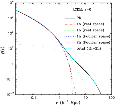
Figure 1 plots the mass two-point correlation function $\xi(r)$ at $z=0$ for the $\Lambda$CDM model. The halo model prediction is shown by the dot-dashed curve, which matches the solid curve given by the fitting formula of Peacock & Dodds (1996; hereafter PD). We consider the NFW profile with the concentration specified by $(c_{0},\beta)=(10,0.2)$ in equation (18) as the fiducial model. During the preparation of this paper, Smith et al. (2002) have proposed a new fitting formula of the non-linear power spectrum that can better match high-resolution $N$-body simulations. For the $\Lambda$CDM model, the effect is small: the power spectrum differs from the PD prediction by $\sim 10\%$ at most at $k\lower 2.15277pt\hbox{$\;\buildrel<\over{\sim}\;$}30h/$Mpc. The thick dashed curve shows the real-space halo model prediction for the 1-halo contribution to $\xi$ computed from equation (42), while the thick dotted curve is the prediction from the Fourier-space halo model. The two halo model predictions are in remarkable agreement for small scales $r\lower 2.15277pt\hbox{$\;\buildrel<\over{\sim}\;$}2~{}h^{-1}{\rm Mpc}$, but deviate slightly at the transition scale of $\sim 2~{}h^{-1}{\rm Mpc}$ between the non-linear and linear regimes. The discrepancy between the real-space and Fourier-space halo models could be ascribed to the boundary condition used in the integration. The thin dashed curve shows the result obtained without using the boundary condition ($u_{m}(x)=0$ for $x>r_{\rm vir}$) in equation (42), implying that the change alters the predictions only on scales $r\lower 2.15277pt\hbox{$\;\buildrel>\over{\sim}\;$}1~{}h^{-1}{\rm Mpc}$. However on these scales the 2-halo term dominates as shown by the thin dotted curve. Hence, to summarize the results in this figure, the real-space halo model can be used to predict the statistical properties of the non-linear density field with the same accuracy as the Fourier-space halo model whose validity has been carefully investigated in the literature (Seljak 2000; Ma & Fry 2000c; Scoccimarro et al. 2001; TJ02).

Figure 2: (a) The left panel shows the dependence of the 1-halo contribution to $\xi(r)$ on the maximum mass cutoff used in the calculation. From top to bottom, the maximum mass is $10^{16}$, $10^{15}$, $10^{14}$, $10^{13}$ and $10^{12}M_{\odot}$. For comparison, the dashed curve denotes the full $\xi(r)$ (1h+2h) for our reference model. (b) In the middle panel, the three solid curves demonstrate the dependence on the inner slope parameter $\alpha$ of the halo profile (see equation (14)). (c) The right panel shows the dependence on the concentration parameter. The result for our fiducial model $(c_{0},\beta)=(10,0.2)$ is shown by the thick solid curve.

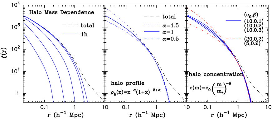
The left panel of Figure 2 shows the dependence on the maximum mass cutoff used in the calculation on $\xi(r)$. From top to bottom, the solid curves show the results for the maximum cutoff of $10^{16}$, $10^{15}$, $10^{14}$, $10^{13}$ and $10^{12}M_{\odot}$. Massive halos with $m\lower 2.15277pt\hbox{$\;\buildrel>\over{\sim}\;$}10^{14}M_{\odot}$ yield the dominant contribution (greater than $\sim 80\%$) to $\xi_{1h}(r)$ for $r\lower 2.15277pt\hbox{$\;\buildrel>\over{\sim}\;$}0.1~{}h^{-1}{\rm Mpc}$, while less massive halos become relevant at smaller scales. The dashed curve denotes the full halo model prediction for $\xi(r)$ (1h+2h) as shown in Figure 1.

The middle and right panels of Figure 2 show the dependences of $\xi(r)$ on the variations in the halo profile. From the middle panel, one can see that increasing $\alpha$ for the halo profile of equation (14) leads to a higher amplitude and steeper slope for $\xi(r)$ on small scales (see also Jain & Sheth 1997; Ma & Fry 2000c). For generic $\alpha$, the angular integration in $\int d^{3}\mbox{{\it\boldmath$s$}}$ in equation (4) is not analytic, so we performed the 3-dimensional integration to get $\xi_{1h}(r)$ numerically. The right panel shows the dependences on the concentration parameter parameterized in terms of the normalization $c_{0}$ and the slope $\beta$ as $c(m)=c_{0}(m/m_{\ast})^{-\beta}$. The result of our fiducial model $(c_{0},\beta)=(10,0.2)$ is shown by the thick solid curve. It is apparent that increasing $c_{0}$ with fixed $\beta$ or decreasing $\beta$ with fixed $c_{0}$ increases $\xi$ at small scales. This is because these variations lead to more concentrated density profiles for halos more massive than the nonlinear mass scale $m_{\ast}$. Since the massive halos dominate the contribution to $\xi$ at the scales considered here, this has the effect of increasing $\xi$. The results in Figure 2 imply that we can adjust the inner slope $\alpha$ and the concentration parameter, both of which are somewhat uncertain theoretically and observationally, so that the halo model can reproduce the PD result for a given mass function (see Seljak 2000 for a similar discussion). We will argue that the 3PCF can be used in combination with the 2PCF to constrain properties of the halo profile.

Figure 3: Comparison between model predictions of the two-point correlation function of the weak lensing convergence field, as in Figure 1. The dashed curve is the real-space halo model prediction (equation 34) for the 1-halo contribution to the 2PCF, while the thick dotted curve denotes the result of the Fourier-space halo model computed from equation (38). The top, broken curve shows the overestimation of the halo model result (1h+2h), if the NFW convergence field in our equation (34) is replaced by Bartelmann’s (1996) result.

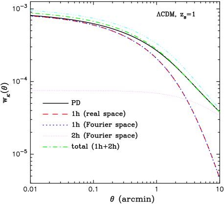
Figure 3 shows the 2PCF of the weak lensing convergence field. The real-space halo model prediction (dashed curve) for the 1-halo contribution is compared with the result of the Fourier-space halo model (thick dotted curve), computed from equations (34) and (38), respectively. Here we have considered the NFW profile and source redshift $z_{s}=1$ for simplicity. The different halo model predictions perfectly agree over the angular scales we have considered. This agreement is encouraging, because the real-space halo approach can then be used to predict the 3PCF with the same accuracy expected as for the Fourier-space model well studied in the literature (TJ02 and references therein). For comparison, the solid curve denotes the PD result and the thin dotted curve is the Fourier-space halo model prediction of the 2-halo term. It clarifies that the 2-halo term is important on $\theta\lower 2.15277pt\hbox{$\;\buildrel>\over{\sim}\;$}3^{\prime}$ for the $\Lambda$CDM model. The dot-dashed curve is the total contribution to the 2PCF from the 1- and 2-halo terms, which slightly deviates from the PD result on the small scales $\theta\lower 2.15277pt\hbox{$\;\buildrel<\over{\sim}\;$}1^{\prime}$. As discussed below equation (28), if we use the expression in Bartelmann (1996) for the NFW convergence field in the calculation of the 1-halo term, one finds discrepancies between the real-space and Fourier-space halo models. The broken curve shows the result (1-halo + 2-halo terms), which overestimates $w_{\kappa}$ by 10-25 % over the scales considered.

4.2 3-point correlation function

4.2.1 Dark matter correlation function

Figure 4: The sketch of the triangle configuration parameterized by $r$, $q$ and $\psi$ used in this paper to describe the 3PCF.

We first consider the 3PCF of the mass density field. To obtain the 1-halo contribution, where all the three matter particles reside in one halo, we perform the following 4-dimensional numerical integration;

$$\zeta_{1h}(r,q,\psi)=\int\!\!dm~{}n(m)\left(\frac{m}{\bar{\rho}_{0}}\right)^{3}\int_{0}^{r_{\rm vir}}\!\!ds\int^{2\pi}_{0}\!\!d\varphi\int^{\pi}_{0}\!\!d\theta~{}s^{2}\sin\theta~{}u_{m}(s)u_{m}(|\mbox{{\it\boldmath$s$}}+\mbox{{\it\boldmath$r$}}|)u_{m}(|\mbox{{\it\boldmath$s$}}+\mbox{{\it\boldmath$q$}}|),$$ (44)

where $|\mbox{{\it\boldmath$s$}}+\mbox{{\it\boldmath$r$}}|=(s^{2}+r^{2}+2sr\cos\theta)^{1/2}$ and $|\mbox{{\it\boldmath$s$}}+\mbox{{\it\boldmath$q$}}|=[s^{2}+q^{2}+2sq(\sin\psi\sin\theta\cos\varphi+\cos\psi\cos\theta)]^{1/2}$. Note that we employ the boundary condition $u_{m}(r)=0$ for $r>r_{\rm vir}$, but this does not affect the final results on the non-linear scales, as explained in Figure 1 and explicitly demonstrated in Figure 8. In the above equation, we have used the fact that the 3PCF can be expressed as a function of the three independent parameters $r$, $q$ and $\psi$ specifying the triangle configuration (see Figure 4).

To complete our halo model predictions, we develop approximations for calculating the 2- and 3-halo terms in Appendix A. The 2-halo term is relevant only for small range of scales in the transition between the quasi-linear and non-linear regimes ($r\sim 1~{}h^{-1}{\rm Mpc}$), while the 3-halo term is dominant on larger scales. As in the literature, we consider the hierarchical 3PCF amplitude defined as

$$Q(r,q,\psi)=\frac{\zeta(r,q,\psi)}{\xi(r)\xi(q)+\xi(r)\xi(|\mbox{{\it\boldmath$r$}}-\mbox{{\it\boldmath$q$}}|)+\xi(q)\xi(|\mbox{{\it\boldmath$r$}}-\mbox{{\it\boldmath$q$}}|)},$$ (45)

where $\zeta=\zeta_{1h}+\zeta_{2h}+\zeta_{3h}$. In the following halo model predictions for $Q$, we will maintain self-consistency by using the halo model for calculating the 2PCF in the denominator of $Q$.

Figure 5: The halo model predictions for the reduced 3PCF, $Q$, as a function of the shapes of triangle configurations. The results for the NFW profile at $z=0$ are plotted for the $\Lambda$CDM model. The triangle shape is parameterized by three parameters $r$, $q$ and $\psi$ as illustrated in Figure 4. The four panels show the results for $Q$ vs. $\psi$, with $r=0.02$, $0.1$, $1.0$ and $10~{}h^{-1}$ Mpc as indicated in the panels. In each panel, the solid, dashed, dot-dashed, dotted, and broken curves denote the $Q$ parameter for $r/q=1$, $2$, $3$, $4$ and $5$, respectively.

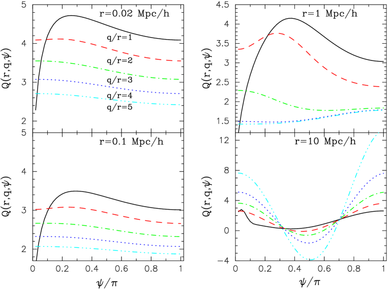
Figure 5 plots the dependences of $Q(r,q,\psi)$ on the size and shape of triangle configurations. In this figure we have used the NFW profile. The four panels show the results for $r=0.02$, $0.1$, $1$ and $10~{}h^{-1}{\rm Mpc}$. In each panel, the solid, dashed, dot-dashed, dotted and broken curves plot the $Q$ values for $q/r=1$, $2$, $3$, $4$ and $5$ as a function of the interior angle $\psi$. It is apparent that on the highly non-linear scales $r\lower 2.15277pt\hbox{$\;\buildrel<\over{\sim}\;$}0.1~{}h^{-1}{\rm Mpc}$ the 3PCF has a weak dependence on the triangle configuration; even so, for plausible halo model parameters the hierarchical form $Q\approx{\rm const.}$ does not hold in that $Q$ depends both on the size and shape of the triangle configuration (also see discussion in Ma & Fry 2000b). The curves with $q/r=1$ show that $Q$ decreases with decreasing $\psi$ at $\psi\lower 2.15277pt\hbox{$\;\buildrel<\over{\sim}\;$}0.2\pi$ because of the strong suppression due to $\xi^{2}$ in the denominator of $Q$. On larger scales $r\lower 2.15277pt\hbox{$\;\buildrel>\over{\sim}\;$}1~{}{\rm Mpc}$, an oscillatory feature in $Q$ appears as predicted by perturbation theory (e.g., Fry 1984b; Barriga & Gaztañaga 2002). Thus, the configuration dependence of the 3PCF is more prominent on quasi-linear scales than on strongly non-linear scales.

Figure 6: The 1-, 2- and 3-halo contributions to the $Q$ parameter are shown by the dashed, dot-dashed and dotted curves, respectively. The triangle shapes are parameterized as in Figure 5. Note that in the top panel the 1-halo term dominates $Q$, while in the bottom panel the 3-halo term dominates.

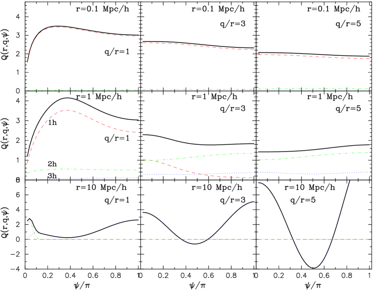
The features observed in $Q$ can be understood using Figure 6, which shows the 1-, 2- and 3-halo contributions to $Q$ separately for the triangle configurations in Figure 5. Note that these separate contributions are shown for the 3PCF, the numerator of $Q$, while the 2PCF factors in the denominator include the full contribution from the 1- plus 2-halo terms. This figure clarifies that the 1-halo term yields the dominant contribution to the 3PCF on small scales $r\lower 2.15277pt\hbox{$\;\buildrel<\over{\sim}\;$}1~{}{\rm Mpc}$. The 2-halo term becomes relevant over the transition scales $1\lower 2.15277pt\hbox{$\;\buildrel<\over{\sim}\;$}r\lower 2.15277pt\hbox{$\;\buildrel<\over{\sim}\;$}5~{}{\rm Mpc}$ between the non-linear and linear regimes, while the 3-halo term dominates for $r\lower 2.15277pt\hbox{$\;\buildrel>\over{\sim}\;$}10~{}{\rm Mpc}$.

Figure 7: Halo model predictions for the reduced 3PCF for equilateral triangles as a function of the side length $r$. The three dashed curves represent the 1-, 2- and 3-halo contributions separately. For comparison, the dotted curve is the perturbation theory result, which matches the 3-halo term on large scales $\lower 2.15277pt\hbox{$\;\buildrel>\over{\sim}\;$}3~{}h^{-1}$Mpc.

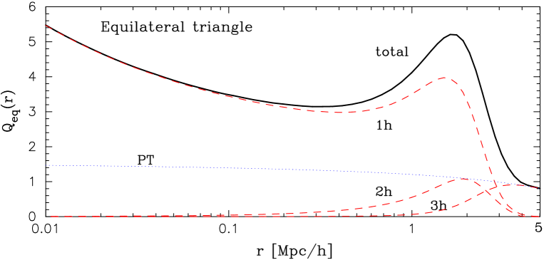
Figure 7 displays the halo model predictions for $Q$ for equilateral triangles as a function of the side length $r$. The three dashed curves plot the 1-, 2- and 3-halo contributions separately. For comparison, the perturbation theory result is shown by the dotted curve. The figure again clarifies that, at the small scales $r\lower 2.15277pt\hbox{$\;\buildrel<\over{\sim}\;$}0.5~{}h^{-1}{\rm Mpc}$, the 1-halo term dominates the total contribution, while the 3-halo term captures the large-scale correlations in the quasi-linear regime. A comparison between the perturbation theory result and the 3-halo term reveals that our approximation (64) reproduces the perturbation theory result at large scales $r\lower 2.15277pt\hbox{$\;\buildrel>\over{\sim}\;$}5~{}h^{-1}{\rm Mpc}$. Thus the way the halo model provides a separate description of the 1-, 2- and 3-halo terms can clarify how gravitational clustering transits from the linear regime to the strongly non-linear regime as one goes to smaller scales.

The halo model predictions match $N$-body simulation results on small scales $r\lower 2.15277pt\hbox{$\;\buildrel<\over{\sim}\;$}1~{}h^{-1}{\rm Mpc}$ (R. Scoccimarro; private communication). However, the $Q$ parameter from the halo model has a bump feature at $r\simeq 2~{}h^{-1}{\rm Mpc}$ which does not seem to be present in simulation data. The corresponding bump feature in the bispectrum has been found at $k\sim 1~{}h{\rm Mpc}^{-1}$ in previous work (see Figure 2 in Scoccimarro et al. 2001 and Figure 13a in Cooray & Sheth 2002). Hence, it is unlikely to be due to inaccuracies in our approximations used for the 2- and 3-halo term calculations, although the approximations tend to overestimate the true amplitudes to some extent as carefully investigated in TJ02. It probably does not reflect real properties of dark matter clustering either (as discussed below for Figure 10). Rather, it can be ascribed to an inaccuracy in the standard implementation of the halo model which appears only on transition scales of order a few Mpc, in contrast to the success of the halo model in the non-linear and linear regimes.

Figure 8: This figure shows the effect of modifying the halo model calculation by altering the halo boundary condition and by exclusion effects in the 2- and 3-halo terms. The upper panel shows how the bump in $Q_{\rm eq}(r)$ is suppressed if halos are not truncated at the virial radius (see text for details). The thick dashed curve shows $Q_{\rm eq}(r)$ and the three thin dashed curves show the 1-, 2- and 3-halo contributions. For comparison, the solid curves are the halo model results shown in Figure 7, in which a sharp cutoff is used at the virial radius. The dot-dashed curve in the lower panel shows the effect on $Q_{\rm eq}(r)$ if halo exclusion effects are included in calculations. The 2-halo term of the 2PCF and the 2- and 3-halo terms of the 3PCF, which enter denominator and numerator in $Q_{\rm eq}(r)$, are constrained by the condition $r_{\rm vir}(m)\leq r/2$. This effect suppresses the amplitudes of the 2- and 3-halo contributions to $Q_{\rm eq}$, again leading to the suppression of the bump feature. The 1-halo term is not shown in this panel as it remains unaffected. The thick dotted curve shows the prediction for $Q_{\rm eq}(r)$ if both boundary and exclusion effects are included.

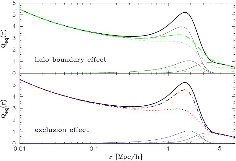
One possible origin of the inaccuracy is the sharp cutoff at the virial radius for the integrals for the 2PCF and 3PCF, as have been used for the real-space halo model in this paper as well as for the Fourier-space model in Scoccimarro et al (2001) and Cooray & Sheth (2002). As shown in Figure 1, modifications of the integration range could alter the halo model prediction at the transition scales. In the upper panel of Figure 8, the thick dashed curve shows the result obtained without using the boundary condition $u_{m}(x)=0$ for $x>r_{\rm vir}$ for the calculations of the 1-halo terms of the 2PCF and 3PCF, which enter the denominator and numerator of $Q$, respectively. One can see that the bump feature is weakened through complex dependences – the 2PCF amplitude is enhanced by the modified boundary condition more strongly than the 3PCF. In fact, this trend is verified by the results in Figure 3 and 4 in Ma & Fry (2000b), which show that the Fourier-space halo model yields bispectra with no bump feature. Ma & Fry employed the Fourier transform of the non-truncated profile, $\tilde{u}_{m}(k)$, calculated over an infinite integration range, which includes mass contribution outside the virial region. However, in this paper we have used the virial boundary condition since it preserves mass conservation. We have also clarified in Figure 3 that, if we include mass contributions beyond the virial radius, the halo model prediction for the lensing 2PCF overestimates the amplitude (see the dot-dashed and broken curves in Figure 3). In reality, the mass distribution outside the virial region eventually merges into quasi-linear structures, such as filamentary structures in the universe, which are relevant for the transition scale ($\delta\lower 2.15277pt\hbox{$\;\buildrel>\over{\sim}\;$}1$), and are unlikely to follow the halo profile far outside the virial region. Therefore, a careful investigation of which boundary conditions to use for the halo model integrals will be needed to achieve more accurate predictions at the transition scale.

Another effect that could be manifested at these scales is the exclusion effect of different halos for the 2- and 3-halo terms. We could impose the condition that different halos are separated by scales larger than the sum of their virial radii. The halo model does not explicitly account for this effect. Since the transition scale $\sim 1\ {\rm Mpc}$ is of the order of the virial radius of massive halos that make a significant contribution to the integrals, the halo model used here might overestimate the contribution from the 2- and 3-halo terms at these scales. The dot-dashed curve in the lower panel of Figure 8 shows an estimate of this effect. The estimate is obtained by imposing the condition $r_{\rm vir}(m)\leq r/2$, an approximate prescription to exclude pairs and triplets of halos contributing to the 2- and 3-halo terms at scales smaller than the sum of their virial radii. The plot shows that including the exclusion effect suppresses the bump feature in $Q$. The dotted curve in the lower panel of Figure 8 shows the result of applying both alterations (boundary and exclusion effects) to the calculations. A systematic resolution of these problems is beyond the scope of our paper, and will be considered elsewhere. Finally, the figure implies that, except for the problematic bump feature, a transition between the non-linear amplitude ($Q\lower 2.15277pt\hbox{$\;\buildrel>\over{\sim}\;$}3$) and the quasi-linear amplitude ($Q\lower 2.15277pt\hbox{$\;\buildrel<\over{\sim}\;$}1$) occurs at scales of a few $h^{-1}{\rm Mpc}$, corresponding to a flattening of the 2PCF $\xi(r)$ (see Figure 1).

Figure 9: The results for $Q_{\rm eq}(r)$ are shown for different cosmological models as in Figure 7. The dotted curve denotes the $\Lambda$CDM model with $\sigma_{8}=1.1$, compared to $\sigma_{8}=0.9$ for our fiducial model. The dashed curve shows the result for the SCDM model. To show the sensitivity of $Q$ to the shape of the matter power spectrum, we also show the result for the $\tau$CDM model, which is different only in the shape parameter ($\Gamma=0.21$) from the SCDM model ($\Gamma=0.5$).

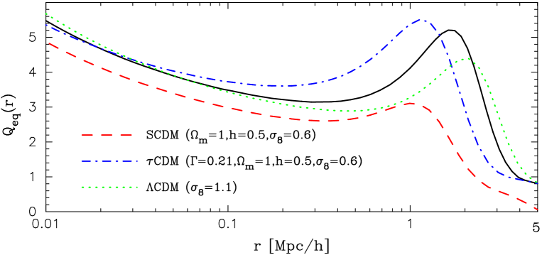
Figure 9 shows the dependences of $Q$ on the cosmological model. We consider three models that differ from our fiducial model. One is the $\Lambda$ CDM model normalized with $\sigma_{8}=1.1$, motivated by the possible detection of the Sunyaev-Zel’dovich effect in the CMB (Bond et al. 2002). The second is a flat model without cosmological constant (SCDM), with parameters $\Omega_{m0}=1$, $h=0.5$ and $\sigma_{8}=0.6$. To clarify the dependence on the shape of the matter power spectrum, we also consider the $\tau$CDM model, where the shape parameter $\Gamma=0.21$, but the other parameters are same as in the SCDM model. The figure reveals that the $Q$ parameter is not very different for the different models but does vary slightly with changes in the various model parameters. Thus accurate measurements must be interpreted with precise predictions that explore all parameter dependences.

Figure 10: Halo model predictions for the dependence of the $Q$ parameter on the triangle shapes parameterized by $r_{12}$, $u$ and $v$ (see equation (46)). The values of $r_{12}$, $u$ and $v$ are the same as those used in Figure 2 in Jing & Börner (1998), where the $Q$ parameters were computed from $N$-body simulations. The data with error bars denote the simulation results.

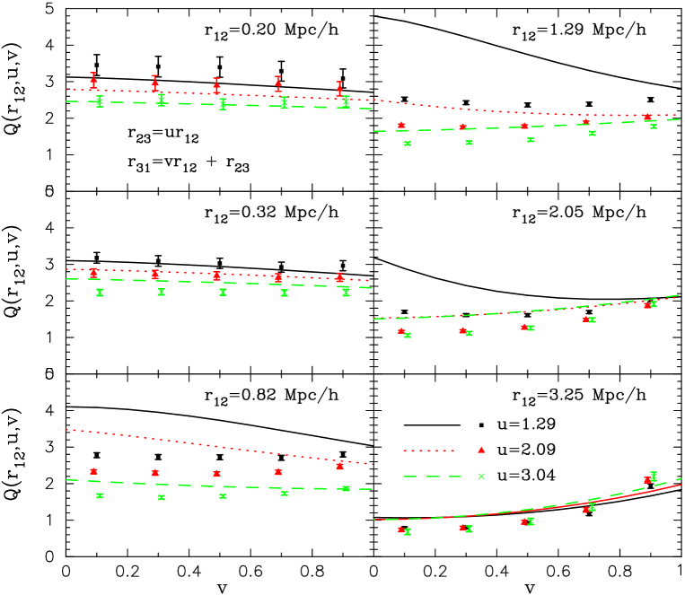
For completeness we present our results with the triangles specified using a set of alternative parameters which have been used in the literature (e.g., Peebles 1980):

$$u\equiv\frac{r_{23}}{r_{12}},\hskip 20.00003ptv\equiv\frac{r_{31}-r_{23}}{r_{12}},$$ (46)

with the condition $r_{12}\leq r_{23}\leq r_{31}$ which imposes the constraints $u\geq 1$ and $0\leq v\leq 1$. The 3PCF for any triangle can then be expressed as a function of three parameters $r_{12}$, $u$ and $v$, where $u$ and $v$ characterize the shape and $r_{12}$ the size of a triangle.

Figure 10 shows the dependence of $Q$ on $r_{12}$, $u$ and $v$. The values of $r_{12}$, $u$ and $v$ are chosen such that our model predictions can be compared with the $N$-body simulation results shown in Figure 2 in Jing & Börner (1998). The data with the error bars represent the simulation results, which were kindly made available to us by Yipeng Jing. Although the cosmological parameters in Jing & Börner (1998) are slightly different from our model, this fact does not matter because of the weak dependence of $Q$ on the cosmological model as explained in Figure 9. It is also noted that the halo model prediction does not account for the effect of averaging over bin widths in $u$ and $r_{12}$ which is taken for the $Q$ measurement from the simulations. This figure reveals that our halo model agrees well with the simulation results for the configuration dependence of $Q$ and its amplitude at the non-linear scales $r_{12}=0.2$ and $0.32~{}h^{-1}$Mpc, as well as the quasi-linear scale $r_{12}=3.25~{}h^{-1}$Mpc. However, as discussed above, for the case in which one side length of the triangle is comparable to $1~{}h^{-1}{\rm Mpc}$, the halo model tends to overestimate the simulation result. More detailed comparisons with recent higher resolution simulations will be presented elsewhere.

Figure 11: The dependence of the mass 3PCF on the maximum mass cutoff used in the halo model calculations, plotted against the side length of the equilateral triangle. From top to bottom, the maximum mass is $10^{16}$, $10^{15}$, $10^{14}$, $10^{13}$ and $10^{12}M_{\odot}$. The dashed curve is the full 3PCF.

Figure 11 shows how the 1-halo contribution to the mass 3PCF depends on the maximum mass cutoff used in the calculation against the side length of equilateral triangles. This can be compared to the dependence of the 2PCF on mass cutoff shown in the left panel of Figure 2. For the 3PCF more massive halos dominate the contribution at a given length scale: for example, at $r=0.5~{}h^{-1}$Mpc, over half the contribution to the 3PCF is from halos with $m>10^{15}M_{\odot}$, whereas for the 2PCF the mass range is $m>10^{14}M_{\odot}$.

Figure 12: The dependences of the $Q$ parameter on the halo profile parameters: the inner slope $\alpha$ and the concentration parameter, $c(m)$, parameterized in terms of the normalization $c_{0}$ at the nonlinear mass scale, and the slope $\beta$. The upper panels show the results for $Q$ versus $\psi$ with the two side lengths $r=q=0.02~{}h^{-1}{\rm Mpc}$ (Figure 4 defines $\psi,r,q$). The lower panels have $r=q/3=0.02~{}h^{-1}{\rm Mpc}$.

Figure 13: The $Q$ values, as in the previous figure, for $r=0.1~{}h^{-1}{\rm Mpc}$.

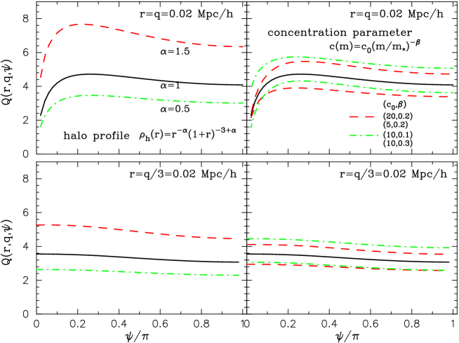
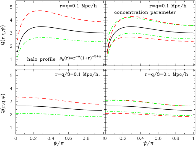
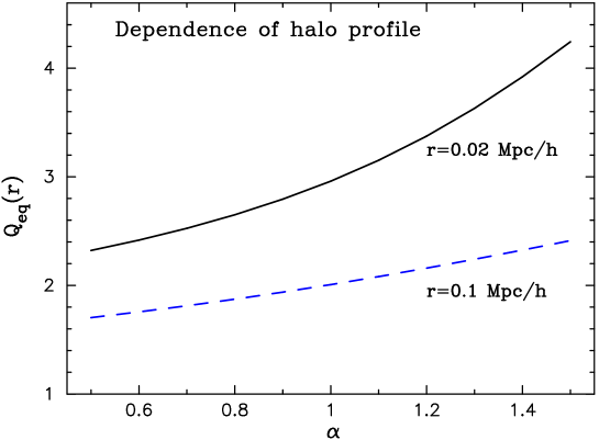
In Figure 12 and 13, we present dependences of the $Q$ parameter on possible variations in the halo inner slope and the concentration parameter, as in the middle and right panels of Figure 2. To do this, we use the parameters $r$, $q$ and $\psi$ for the triangle configuration as in Figure 5. Note that the results shown are computed from only the 1-halo contributions to the 3PCF and 2PCF, which enter the numerator and denominator of $Q$, respectively, since the variations of the halo profile are relevant only at the non-linear scales. Increasing the inner slope parameter $\alpha$ for the profile (14) leads to higher $Q$ (see similar discussions in Ma & Fry 2000a for the bispectrum). A comparison of Figures 12 and 13 shows that $Q$ is more sensitive to $\alpha$ for triangles with smaller size. Compared with the effect on the 2PCF shown in Figure 2, this result also means that the 3PCF is more sensitive to the inner slope of halo profile than the 2PCF. We find the following fitting formula of the dependence of the 2PCF and the 3PCF on $\alpha$, applicable over the range $0.5\leq\alpha\leq 1.5$;

$$\xi^{2}(r)=[\xi_{NFW}^{2}]^{1+0.017(\alpha-1)+0.074(\alpha^{2}-1)},\hskip 5.0pt\zeta(r)=\zeta_{NFW}{}^{1+0.021(\alpha-1)+0.08(\alpha^{2}-1)},\hskip 5.0ptQ=Q_{NFW}{}^{1+0.094(\alpha-1)+0.24(\alpha^{2}-1)}\hskip 20.00003pt$$ (47)

for $r=0.02~{}h^{-1}{\rm Mpc}$, while

$$\xi^{2}(r)=[\xi_{NFW}^{2}]^{1+0.048(\alpha-1)+0.034(\alpha^{2}-1)},\hskip 5.0pt\zeta(r)=\zeta_{NFW}{}^{1+0.06(\alpha-1)+0.033(\alpha^{2}-1)},\hskip 5.0ptQ=Q_{NFW}{}^{1+0.38(\alpha-1)+0.057(\alpha^{2}-1)}\hskip 20.00003pt$$ (48)

for $r=0.1~{}h^{-1}{\rm Mpc}$. Here $\xi_{NFW}$, $\zeta_{NFW}$ and $Q_{NFW}$ denote the use of the NFW profile ($\alpha=1$); we have used equilateral triangle configurations for the 3PCF calculation. Figure 14 explicitly plots the $\alpha$ dependence of $Q$.

Figure 14: The $Q$ parameter for equilateral triangles as a function of the inner slope parameter $\alpha$ for the halo density profile given by equation (14). The solid and dashed curves are the results for $r=0.02$ and $0.1~{}h^{-1}$Mpc, respectively.

The right panels in Figure 12 and 13 illustrate the sensitivity of $Q$ to possible variations in the halo concentration parameter (18). One can see that the change in concentration affects the $Q$ amplitudes, but does not strongly alter the configuration dependence. Increasing $c_{0}$ with fixed $\beta$ or decreasing $\beta$ with fixed $c_{0}$ leads to a higher amplitude for $Q$, which is the same trend as for the 2PCF shown in Figure 2. This implies that the 3PCF is more sensitive to the halo concentration than the 2PCF. These results in Figure 12 and 13 show that measuring the 3PCF could constrain halo profile properties complementary to the measurements of the 2PCF, in analogy with determinations of the galaxy bias parameter from measurements at quasi-linear scales (Feldmann et al. 2001; Verde et al. 2002).

In Figure 12-14, we have demonstrated the sensitivity of the mass 3PCF to the halo profile properties. We have compared our halo model predictions for $Q$ with the asymptotic shape derived in Ma & Fry (2000b) based on the halo model. The asymptotic $Q$ amplitude depends only on the mass slope $\beta$ of the concentration parameter (see equation (18)), the slope $\alpha^{\prime}$ in the low mass end of the mass dependence of the mass function, $n(m)\propto\nu^{\alpha^{\prime}}$, and a primordial spectral index $n$. From equation (7) in Ma & Fry (2000b), the asymptotic $Q$ for equilateral triangles is given by

$$Q(r)\propto r^{-\gamma},\hskip 10.00002pt\gamma=\frac{\alpha^{\prime}(n+3)}{2(3\beta^{\prime}+1)},$$ (49)

where $\beta^{\prime}\approx 0.8\beta$ and we have considered equilateral triangle configuration. This equation was derived under three assumptions: the contribution from the exponential cutoff of the mass function in the high mass end was ignored, a scale-free primordial power spectrum was employed and the $k$-dependence of the Fourier-transformed halo profile, $\tilde{u}_{m}(k)$ was ignored. The third assumption leads to the consequence that the asymptotic $Q$ has no dependence on the inner slope of the halo profile. Since for the profile in equation (14) $\tilde{u}_{m}(k)$ does depend on the inner slope as $\tilde{u}_{m}(k)\approx 1$ and $\propto k^{-3+\alpha}$ for $k\ll c/r_{\rm vir}$ and $k\gg c/r_{\rm vir}$, the asymptotic $Q$ should depend on the inner slope or more generally the halo profile shape. By comparing our predictions of $Q$ with the analytical result of Ma & Fry (2000b), we find that our halo model predicts a steeper slope for $Q(r)$ than expected from the asymptotic shape in equation (49), for plausible values of $\beta$ and $\alpha^{\prime}$.

This discrepancy is probably due to the assumptions used in analytically deriving the asymptotic shape. The $r$-dependence of $Q$ arises from a complex superposition of contributions from the halo profile, the power spectrum shape and the shape of the mass function. Indeed, as an example of this possibility, Taruya, Hamana & Kayo (2002) explicitly showed, based on the halo model, that the non-Gaussian tail of the probability distribution function of the density field arises from such a superposition for small smoothing scales.

An important implication pointed out in Ma & Fry (2000b,c) is that plausible halo model properties are unlikely to follow the stable clustering hypothesis. This hypothesis is useful because it allows us to analytically predict the behavior of non-linear gravitational clustering (e.g. Peebles 1980; Jain 1997). In fact, the popular PD fitting formula widely used in the literature was derived based on this hypothesis (also see Hamilton et al. 1991; Jain, Mo & White 1995). Very recently, Smith et al. (2002) showed that the non-linear power spectra measured from the high-resolution $N$-body simulations indeed showed a weak violation of the stable clustering hypothesis. Figure 9 in Smith et al. (2002) compares the $k$-slope of the measured non-linear power spectrum with the asymptotic prediction from Ma & Fry (2000b), which also shows some discrepancies. Hence, a careful investigation will be needed to clarify how non-linear gravitational clustering can be described by the halo model ingredients in connection with the stable clustering hypothesis and the hierarchical ansatz (see also the next subsection).

4.2.2 The hierarchy of higher-order correlation functions

As stated in §2.1, the real-space halo model can be a useful tool for predicting the $n$-point correlation functions in the strongly non-linear regime, where correlations within one halo dominate the contribution to the $n$-point functions. The exact expressions for the the hierarchy are provided by the BBGKY equations (Peebles 1980), which govern collisionless gravitational system. However, their complex form makes it intractable to obtain solutions for the higher order correlations in the non-linear regime. Here we will use the halo model to shed some light on a fundamental question about gravity that has been discussed in the literature over the last decades: what is the asymptotic small-scale behavior of the hierarchy of the $n$-point functions under gravitational clustering (e.g., Peebles 1980; Fry 1984a,b; Hamilton 1988; Ma & Fry 2000b; Bernardeau et al. 2002a)?

The reduced $n$-point correlation function, $Q_{n}$, is defined as

$$Q_{n}\equiv\frac{\xi^{(n)}(\mbox{{\it\boldmath$r$}}_{1},\dots,\mbox{{\it\boldmath$r$}}_{n})}{\Sigma_{{\rm labelings}}\Pi_{{\rm edges}~{}ij}^{n-1}\xi({r_{ij}})},$$ (50)

where the denominator is given by all topologically distinct tree diagrams (the different $n^{n-2}$ ways of drawing $(n-1)$ links that connect $n$ points). This form is motivated by the expectation $\xi^{(n)}\propto\xi^{n-1}$, indicated observationally by the pioneering measurements of the two- and three-point functions from galaxy surveys (e.g., Groth & Peebles 1977; Peebles 1980), and theoretically by perturbation theory (Fry 1984b). The amplitudes $Q_{n}$ are a natural set of statistics to describe the non-Gaussianity that results from gravitational clustering.

Figure 15: The hierarchical amplitude $Q_{n}$ for the mass $n$-point correlation function in the strongly non-linear regime is shown versus the order $n$. We consider the configuration with $n$ equal sides of length $r=0.1h^{-1}$Mpc and equal interior angles. The solid curve shows the halo model prediction. The dashed curve shows the scaling for $Q_{n}$ as a function of $Q_{3}$ and $n$ proposed by Fry (1984a), while the dotted curve shows the formula proposed in Hamilton (1988) (we have used the halo model result for $Q_{3}$ in these formulae). The dot-dashed curve is the prediction from hyper-extended perturbation theory (Scoccimarro & Frieman 1999).

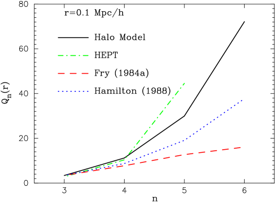
The solid curve in Figure 15 shows the halo model predictions for the hierarchical amplitudes $Q_{n}$ for $3\leq n\leq 6$. We consider configurations with $n$ equal sides, each of length $r=0.1h^{-1}$Mpc, and equal interior angles for evaluations of the $n$-point functions. We take the halo profile to have the NFW form. For comparison, the dashed curve shows the scaling law for $Q_{n}$ proposed in Fry (1984a): $Q_{n}=(4Q_{3}/n)^{(n-2)}n/(2n-2)$. The dotted curve shows the scaling suggested by Hamilton (1988): $Q_{n}=(Q_{3}/n)^{n-2}n!/2$. The dot-dashed curve is the prediction from hyper-extended perturbation theory for $3\leq n\leq 5$ (Scoccimarro & Frieman 1999). The halo model predicts stronger clustering with increasing $n$ than the formulae of Fry and of Hamilton, but not as strong as hyper-extended perturbation theory. Note that higher-order correlations are more sensitive to variations in the inner slope and halo concentrations of massive halos.

The results in Figure 15 might be compared with Figure 3 in Szapudi et al. (1999), which show the cumulants $S_{n}$ ($3\leq n\leq 10$) measured from the $N$-body simulations. From equation (50) we can expect following rough relation between the cumulants and the reduced $n$-point correlation functions:

$$S_{n}(r)\approx\frac{\xi^{(n)}(r)}{\left[\xi^{(2)}(r)\right]^{(n-1)}}\sim n^{n-2}~{}Q_{n}(r).$$ (51)

Table 1: Comparison of the theoretical predictions for the cumulants, $S_{n}$, at $r=0.1h^{-1}$Mpc with the simulation result. The analytical predictions are estimated from the reduced $n$-point functions, $Q_{n}$, shown in Figure 15 using equation (51). The simulation results correspond to the values denoted by the dashed curves in Figure 3 in Szapudi et al (1999), which are measured from $N$-body simulations for the SCDM model.

	$S_{3}$	$S_{4}$	$S_{5}$	$S_{6}$
Halo Model	10	180	$3.7\times 10^{3}$	$9.3\times 10^{4}$
HEPT (Scoccimarro & Freeman 1999)	8.4	166	$5.6\times 10^{3}$	-
Fry 1984a	10	124	$1.6\times 10^{3}$	$2.1\times 10^{4}$
Hamilton 1988	10	139	$2.4\times 10^{3}$	$4.9\times 10^{4}$
$N$-body simulation in Szapudi et al. 1999	$\sim 10$	$\sim 300$	$\sim 10^{4}$	$\sim 4\times 10^{5}$

Table 1 shows a comparison of the simulation results for $S_{n}$ in Szapudi et al. (1999) with the theoretical predictions scaled from the values of $Q_{n}$ in Figure 15. Note that the simulation results were read from the dashed curves in Figure 3 in Szapudi et al. (1999) for the SCDM model (the cosmological parameters are slightly different from the model we have considered), and we expect similar values for the $\Lambda$CDM because of the weak dependence of $S_{n}$ on cosmological models. One can see that the rapid increase in the amplitudes of $S_{n}$ with $n$ seen in the simulation result is better described by the halo model predictions than those of Fry and of Hamilton. However, as explicitly pointed out in Szapudi et al. (1999), the simulation results might be overestimated due to the shot noise effect. Therefore, further detailed work is needed to systematically explore the consistency of the halo model with gravitational dynamics.

4.2.3 The 3-point correlation function of galaxies

It is straightforward to extend the dark matter halo approach to calculate the 3PCF of galaxies which can be measured from galaxy surveys. To do this, we need to know the mean number of galaxies per halo of given mass, known as the halo occupation number, $\langle{N_{\rm gal}}\rangle(m)$, and the second and third moments of the galaxy distribution ($\langle{N_{\rm gal}(N_{\rm gal}-1)}\rangle$ and $\langle{N_{\rm gal}(N_{\rm gal}-1)(N_{\rm gal}-2)}\rangle$). Following the method in Scoccimarro et al. (2001), the real-space halo model expressions for the 1-halo contributions to the galaxy 2PCF and 3PCF are given by

$$\xi^{\rm gal}_{1h}(r) = 2\pi\int\!\!dm~{}n(m)\frac{\langle{N_{\rm gal}(N_{\rm gal}-1)}\rangle}{\bar{n}_{\rm gal}^{2}}\int_{0}^{r_{\rm vir}}\!\!ds\int^{\pi}_{0}\!\!d\theta~{}s^{2}\sin\theta~{}u_{m}(s)u_{m}(|\mbox{{\it\boldmath$s$}}+\mbox{{\it\boldmath$r$}}|),$$

$$\zeta^{\rm gal}_{1h}(r,q,\psi) = \int\!\!dm~{}n(m)\frac{\langle{N_{\rm gal}(N_{\rm gal}-1)(N_{\rm gal}-2)}\rangle}{\bar{n}_{\rm gal}^{3}}\int_{0}^{r_{\rm vir}}\!\!ds\int^{2\pi}_{0}\!\!d\varphi\int^{\pi}_{0}\!\!d\theta~{}s^{2}\sin\theta~{}u_{m}(s)u_{m}(|\mbox{{\it\boldmath$s$}}+\mbox{{\it\boldmath$r$}}|)u_{m}(|\mbox{{\it\boldmath$s$}}+\mbox{{\it\boldmath$q$}}|),$$ (52)

where $\bar{n}_{g}$ denotes the mean number density of galaxies defined as

$$\bar{n}_{g}=\int\!\!dm~{}n(m)\langle{N_{\rm gal}}\rangle(m).$$ (53)

In a similar manner, we can derive halo model predictions for the 2-halo contribution to the galaxy 2PCF, and the 2- and 3-halo contributions to the galaxy 3PCF. For simplicity we assume that the distribution of galaxies within a given halo follows the dark matter profile $u_{m}(r)$. Note that in the large-scale limit, the galaxy bias parameter is defined as

$$b_{g}=\frac{1}{\bar{n}_{g}}\int\!dm~{}n(m)b(m)\frac{\langle{N_{\rm gal}}\rangle(m)}{m}.$$ (54)

The halo occupation number has been used in the literature to explain galaxy clustering properties (Jing, Mo & Börner 1998; Seljak 2000; Peacock & Smith 2000; Scoccimarro et al. 2001; Sheth et al. 2001; Berlind & Weinberg 2002; Moustakas & Somerville 2001; Scranton 2002; Cooray 2002). In this paper, we employ the model of Scranton (2002), which approximately reproduces the results for $\langle{N_{\rm gal}}\rangle(m)$ from semi-analytic models in Kauffmann et al. (1999). The model gives $\langle{N_{\rm gal}}\rangle$ for red and blue galaxies

$$\langle{N_{\rm gal}}\rangle(m)=\left\{\begin{array}[]{ll}\left(\frac{m}{m_{R}}\right)^{\gamma_{R}}e^{-(m_{R0}/m)^{1/2}}&\mbox{for red galaxies},\\ \left(\frac{m}{m_{B}}\right)^{\gamma_{B}}+Ae^{-A_{0}\left(\log m-m_{B_{s}}\right)^{2}}&\mbox{for blue galaxies}\end{array}\right.$$ (55)

where the parameters $\gamma_{R}=1.1$, $m_{R}=1.8\times 10^{13}h^{-1}M_{\odot}$ and $m_{R0}=4.9\times 10^{12}h^{-1}M_{\odot}$ for red galaxies, while $\gamma_{B}=0.93$, $m_{B}=2.34\times 10^{13}h^{-1}M_{\odot}$, $A=0.65$, $A_{0}=6.6$ and $m_{B_{s}}=11.73$ for blue galaxies. In the following, we employ a lower mass cutoff of $m\geq 10^{11}~{}h^{-1}M_{\odot}$ for the calculations, since in small halos effects such as supernova winds can blow away the gas from halos and thus suppresses further star formation. The model above yields bias parameters $b_{g,{\rm red}}=1.51$ and $b_{g,{\rm blue}}=0.82$ for red and blue galaxies, respectively.

Figure 16: Mean number of red and blue galaxies as a function of parent halo mass using the forms in equation (55). The thin dashed curve shows the model for blue galaxies without the bump feature, which we will use to demonstrate the effect on the halo model prediction for the 3PCF in Figure 18.

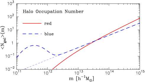
Figure 16 plots the mean number of galaxies, $\langle{N_{\rm gal}}\rangle(m)$, as a function of parent halo mass. The figure shows that $\langle{N_{\rm gal}}\rangle\leq 1$ at $m\lower 2.15277pt\hbox{$\;\buildrel<\over{\sim}\;$}10^{13}~{}h^{-1}M_{\odot}$ for both types of galaxies; a significant fraction of low mass halos are thus likely to contain at most one galaxy. For such low mass halos, we need to carefully model the higher order moments of the galaxy distribution within them, as discussed below. It is also apparent that $\langle{N_{\rm gal}}\rangle$ for blue galaxies has a bump feature for halos of $m\lower 2.15277pt\hbox{$\;\buildrel<\over{\sim}\;$}10^{12}~{}h^{-1}M_{\odot}$. The bump is due to the prescriptions used in the semi-analytical model. Although stars are formed from the cold gas in halos within a dynamical time scale, it is assumed that the gas cooling in halos with circular velocity $V_{c}>350$ km s^-1 does not form visible stars so that the output galaxy catalog can fit the observed Tully-Fisher relation (see Kauffmann et al. 1999 for details). This sharp cutoff of the star formation prevents further formation of galaxies in halos with $V_{c}>350$ km s^-1 unless the halos experience merging, which is taken as the trigger to induce the starburst. Note that the circular velocity $V_{c}=350$km s^-1 roughly corresponds to halo of $m\sim 10^{13}M_{\odot}$ at the present epoch; the velocity is larger for the same mass halo at earlier epochs. In fact, we will show that the bump feature drastically affects the configuration dependence and amplitude of the reduced 3PCF of blue galaxies.

As mentioned above, we also need the second and third moments of the galaxy distribution within parent halos, $\langle{N_{\rm gal}(N_{\rm gal}-1)}\rangle$ and $\langle{N_{\rm gal}(N_{\rm gal}-1)(N_{\rm gal}-2)}\rangle$. We follow Scranton (2002), who expressed them as $\langle{N_{\rm gal}(N_{\rm gal}-1)}\rangle\approx\alpha_{g}^{2}(m)\langle{N_{\rm gal}}\rangle^{2}$ and $\langle{N_{\rm gal}(N_{\rm gal}-1)(N_{\rm gal}-2)}\rangle\approx\alpha_{g}^{3}(m)\langle{N_{\rm gal}}\rangle^{3}$, where

$$\alpha_{g}(m)=\left\{\begin{array}[]{ll}1&m>10^{13}h^{-1}M_{\odot},\\ \ln(\sqrt{m/10^{11}h^{-1}M_{\odot}})&m<10^{13}h^{-1}M_{\odot}.\end{array}\right.$$ (58)

This model implies that galaxies follow a Poisson distribution for massive halos $m\lower 2.15277pt\hbox{$\;\buildrel>\over{\sim}\;$}10^{13}h^{-1}M_{\odot}$ and a sub-Poisson distribution for smaller halos. Other treatments of the sub-Poisson distribution have been proposed by Sheth et al. (2001) and Scoccimarro et al. (20001).

We expect that the models of the 2nd and 3rd moments of $N_{\rm gal}(m)$ will affect $Q_{\rm gal}$ at small scales which are dominated by the 1-halo term. Large scales $\lower 2.15277pt\hbox{$\;\buildrel>\over{\sim}\;$}5~{}h^{-1}$Mpc, in the quasi-linear regime, are dominated by the 3-halo term. The behavior of $Q_{\rm gal}$ on the large scales can be roughly expressed in terms of the bias parameter (54) as $Q_{\rm gal}\sim Q_{\rm mass}/b_{g}$. This follows from $Q_{\rm gal}\sim\zeta_{\rm gal}/(3\xi_{\rm gal}^{2})$ and that: $\zeta_{\rm gal}\sim b_{g}^{3}\zeta_{\rm mass}$ and $\xi_{\rm gal}\sim b_{g}^{2}\xi_{\rm mass}$. As a result, the anti-biasing and bias of blue and red galaxies should lead to larger or smaller amplitudes of $Q_{\rm gal}$ compared to $Q_{\rm mass}$, respectively.

Figure 17: Halo model predictions for the galaxy 3PCF as a function of triangle shapes parameterized by $r$, $q$ and $\psi$ (see Figure 4). The solid, dashed and dotted curves show the results for the mass and for blue and red galaxies, respectively. We have employed the model of equation (55) for the the halo occupation number of red and blue galaxies.

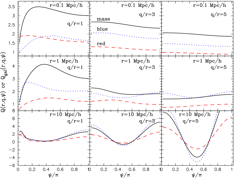
Figure 17 shows $Q_{\rm gal}$ for the galaxy 3PCF with triangle configurations parameterized by $r$, $q$ and $\psi$ as in Figure 5. For red galaxies, the halo model combined with the halo occupation number leads to a weaker configuration dependence and smaller amplitude for $Q_{\rm gal}$ than the mass 3PCF, as suggested from the measurements in Jing & Börner (1998). On the other hand, the 3PCF of blue galaxies displays complex features. This is mainly due to the bump feature in $\langle{N_{\rm gal}}\rangle(m)$ at $10^{11}\leq m\lower 2.15277pt\hbox{$\;\buildrel<\over{\sim}\;$}10^{13}~{}h^{-1}M_{\odot}$, as shown below. Hence, a detailed knowledge of the configuration dependence of $Q_{\rm gal}$ could be used to quantitatively constrain the occupation number, or more generally, the galaxy formation scenario as a function of observed galaxy properties (morphology, luminosity and so on) within a halo of given mass.

Figure 18: The upper panel shows the reduced 3PCF of red (dashed curves) and blue (dotted curves) galaxies as a function of the side length of equilateral triangles, as in Figure 7. The thin curves show the 1-, 2- and 3-halo contributions separately. For comparison, the solid curve shows the result for the mass 3PCF. Note that the bias parameters are $b_{g,{\rm red}}=1.51$ and $b_{g,{\rm blue}}=0.82$ for the red and blue galaxies, respectively. The lower panel explores the dependence of $Q_{\rm gal}$ for blue galaxies on the model ingredients. The dot-dashed curve shows the result for the $Q_{\rm gal}$ of blue galaxies, if we suppress the bump feature in $\langle{N_{\rm gal}}\rangle(m)$ at $10^{11}\leq m\lower 2.15277pt\hbox{$\;\buildrel<\over{\sim}\;$}10^{13}~{}h^{-1}M_{\odot}$ for the calculation. The thin dotted curve shows how the model of Scoccimarro et al. (2001) for the sub-Poisson distribution of blue galaxies changes the prediction at $r\lower 2.15277pt\hbox{$\;\buildrel<\over{\sim}\;$}0.2~{}h^{-1}$Mpc.

Figure 19: The 3PCF (left) and 2PCF (right) of mass, red and blue galaxies.

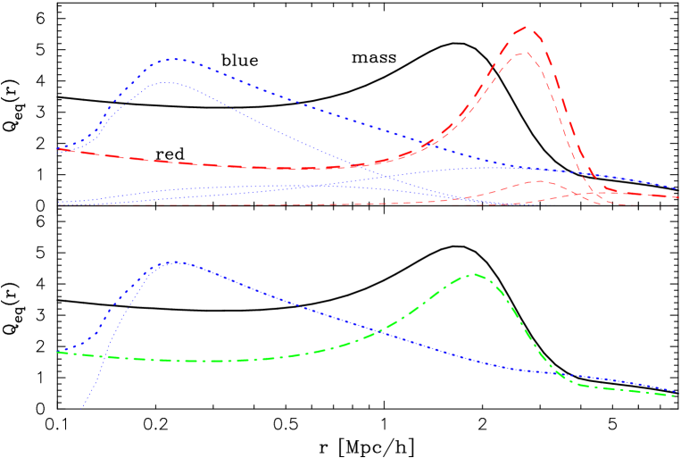
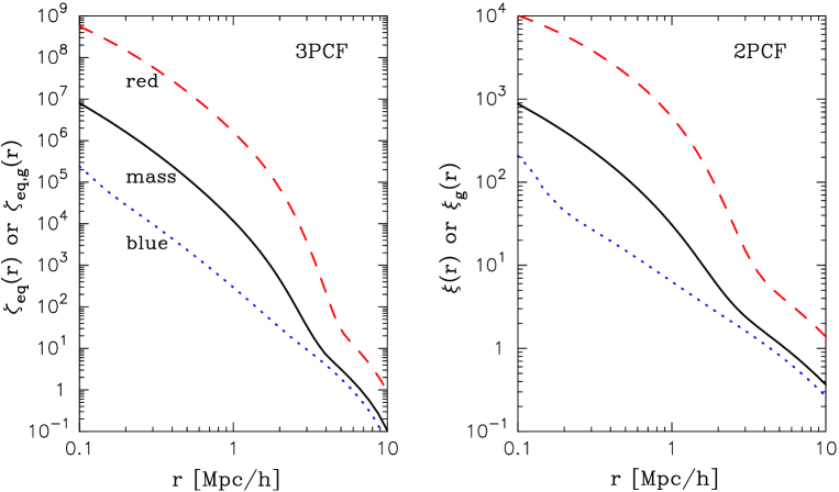
The sensitivity of the input model of the halo occupation number to the galaxy 3PCF can be more clearly understood from Figure 18, which shows the $Q_{\rm gal}$ parameters for equilateral triangles. The 1-, 2- and 3-halo contributions to the galaxy 3PCF are explicitly shown. This figure may be compared with the result for the galaxy bispectrum shown in Figure 6 of Scoccimarro et al. (2001). It is again apparent that the amplitude of $Q_{\rm gal}$ for red galaxies is suppressed compared to the mass 3PCF, while the result for blue galaxies exhibits complex features. Figure 19 shows halo model predictions for the 2PCF and 3PCF of mass and blue and red galaxies separately. It is worth noting that the 2PCF and 3PCF of blue galaxies are well approximated by power laws at scales $r\lower 2.15277pt\hbox{$\;\buildrel>\over{\sim}\;$}0.2~{}h^{-1}$Mpc, unlike the case for the mass or for red galaxies. This is due to the fact that galaxy formation is inefficient in massive halos and thus suppresses the 1-halo term for blue galaxies compared to the mass or to red galaxies which are formed by mergers. Also, $Q_{\rm gal}$ for blue galaxies has contributions from the 2- and 3-halo terms over a wider range of scales compared to that of red galaxies. This is mainly due to the bump feature in $\langle{N_{\rm gal}}\rangle$ at low mass scales in Figure 16, and partly due to the shallower mass slope in $\langle{N_{\rm gal}}\rangle\propto m^{\gamma}$.

The lower panel of Figure 18 explores the origin of the complex features in $Q_{\rm gal}$ for blue galaxies at $0.1\lower 2.15277pt\hbox{$\;\buildrel<\over{\sim}\;$}r\lower 2.15277pt\hbox{$\;\buildrel<\over{\sim}\;$}2~{}h^{-1}$Mpc. The dot-dashed curve shows how the halo model prediction for $Q_{\rm gal}$ for blue galaxies changes if we suppress the bump feature in $\langle{N_{\rm gal}}\rangle$ at low mass scales by setting $A=0$ in equation (55). The model $\langle{N_{\rm gal}}\rangle$ used is shown by the thin dashed curve in Figure 16. One can see that the complex features in $Q_{\rm gal}$ disappear, except for the problematic bump feature at $r\sim 2$Mpc (see the discussion around Figure 8), and its amplitude becomes smaller than the mass 3PCF because of the change of the bias parameter to $b_{\rm g}=1.24$ from $b_{\rm g}=0.82$, which results in behavior similar to the red galaxies. Thus, the input model of $\langle{N_{\rm gal}}\rangle$ has a drastic effect on $Q_{\rm gal}$. We also investigate how the halo model predictions are affected by altering the sub-Poisson distribution for the galaxy third-order moment, which is relevant for the range $\langle{N_{\rm gal}}\rangle\leq 1$ or equivalently $m\lower 2.15277pt\hbox{$\;\buildrel<\over{\sim}\;$}10^{13}~{}h^{-1}M_{\odot}$. Scoccimarro et al. (2001) proposed the binomial distribution, where the third-order moments is given by $\langle{N_{\rm gal}(N_{\rm gal}-1)(N_{\rm gal}-2)}\rangle=\alpha_{g}^{2}(2\alpha_{g}^{2}-1)\langle{N_{\rm gal}}\rangle^{3}$. Note that this model leads to negative values for the third moment for $\alpha_{g}\ll 1$. The thin dotted curve in Figure 18 shows the result of using this prescription — it changes $Q_{\rm gal}$ only for scales $r\lower 2.15277pt\hbox{$\;\buildrel<\over{\sim}\;$}0.2~{}h^{-1}$Mpc.

4.3 The 3-point correlation function of weak lensing fields

Next we consider the halo model predictions for the angular 3PCF of the weak lensing convergence field. It should be noted that the following method can be easily extended to the predict the angular 3PCF of the galaxy distribution, as discussed in §3.

The 1-halo term for the 3PCF of $\kappa$ is given by the following 4-dimensional integral:

$$Z_{1h}(r,q,\psi)=\int^{\chi_{s}}_{0}\!\!d\chi~{}d_{A}^{2}(\chi)\int\!\!dm~{}n(m;\chi)\int^{\theta_{\rm vir}}_{0}\!\!d\theta\int^{2\pi}_{0}\!\!d\varphi~{}\theta\ \kappa_{m}(\theta)\kappa_{m}(|\mbox{{\it\boldmath$\theta$}}+\mbox{{\it\boldmath$r$}}|)\kappa_{m}(|\mbox{{\it\boldmath$\theta$}}+\mbox{{\it\boldmath$q$}}|),$$ (59)

where $|\mbox{{\it\boldmath$\theta$}}+\mbox{{\it\boldmath$r$}}|=(\theta^{2}+r^{2}+2\theta r\cos\psi)^{1/2}$ and $|\mbox{{\it\boldmath$\theta$}}+\mbox{{\it\boldmath$q$}}|=(\theta^{2}+q^{2}+2\theta q\cos(\varphi-\psi))^{1/2}$. For the NFW profile, $\kappa_{m}$ is analytically given by equations (28) and (33). Note that $r$ and $q$ denote angular scales, although we use the same notations as for the 3D case for simplicity. In analogy with equation (45), the $Q$ parameter for the angular 3PCF is defined as

$$Q_{\kappa}(r,q,\psi)=\frac{Z(r,q,\psi)}{w_{\kappa}(r)w_{\kappa}(q)+w_{\kappa}(r)w_{\kappa}(|\mbox{{\it\boldmath$r$}}-\mbox{{\it\boldmath$q$}}|)+w_{\kappa}(q)w_{\kappa}(|\mbox{{\it\boldmath$r$}}-\mbox{{\it\boldmath$q$}}|)},$$ (60)

where $Z=Z_{1h}+Z_{2h}+Z_{3h}$. Note that the 2- and 3-halo terms, $Z_{2h}$ and $Z_{3h}$, are computed from the approximations of equations (66) and (67), respectively.

Figure 20: Halo model predictions for the reduced $Q$ parameter for the weak lensing convergence, with triangle configurations parameterized as in Figure 5. The configuration dependence of $Q$ changes as one shifts from the strongly nonlinear regime shown in the left panel to the quasi-linear regime shown in the right panel.

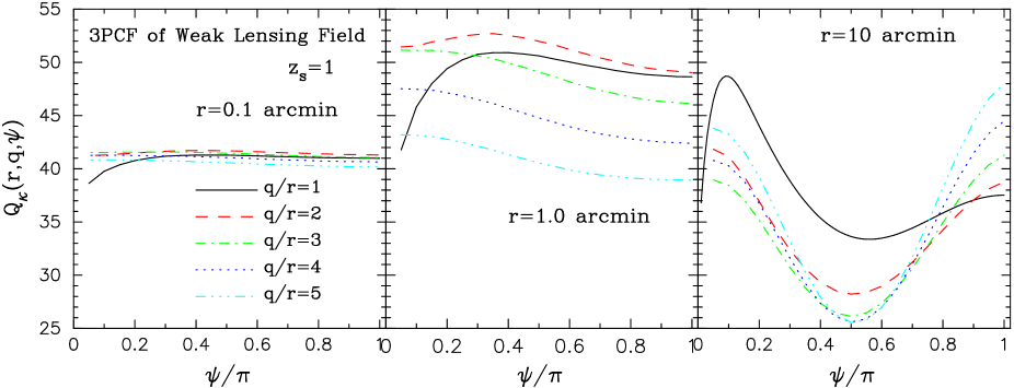
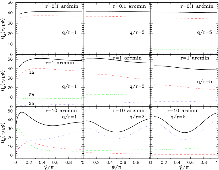
Figure 20 shows halo model predictions for $Q_{\kappa}$ with triangle configurations parameterized as in Figure 5. The halos are taken to have NFW profiles. The hierarchical ansatz, $Q_{\kappa}={\rm const.}$, does not hold rigorously over the scales we have considered, as in the 3D case. However, the configuration dependence of $Q_{\kappa}$ for $r=0.1^{\prime}$ is much weaker than for $r=1^{\prime}$ and $10^{\prime}$. The strong configuration dependence in the two panels on the right can be understood as follows. First, the results in Figure 5 show that the $Q$ parameter for the 3D mass distribution has a stronger configuration dependence for $r\lower 2.15277pt\hbox{$\;\buildrel>\over{\sim}\;$}1~{}h^{-1}$Mpc than on strongly non-linear scales. The weak lensing convergence is a weighted projection of the mass distribution. As a result of the lensing projection, a range of 3-dimensional length scales contributes to $Q_{\kappa}$ at a given $\theta$, which is therefore more sensitive to the 2- and 3-halo terms than the 3D case. This is explicitly shown in Figure 21, which plots the 1- and 2- and 3-halo contributions to $Q_{\kappa}$ for the triangle shapes in Figure 20. For the smallest scale, $r=0.1^{\prime}$, the 1-halo term indeed yields the dominant contribution to $Q_{\kappa}$, but the 2-halo term still has a non-negligible contribution ($\sim 10\%$). For $r=1^{\prime}$, the 2-halo term becomes important ($\lower 2.15277pt\hbox{$\;\buildrel>\over{\sim}\;$}20\%$ contribution). The 3-halo term becomes dominant at for $r\lower 2.15277pt\hbox{$\;\buildrel>\over{\sim}\;$}10^{\prime}$, at which $Q_{\kappa}$ displays a characteristic, oscillatory feature as predicted by perturbation theory.

Figure 21: The 1-, 2- and 3-halo contributions to the $Q$ parameter are shown for the convergence, with triangle shapes parameterized as in Figure 20.

Figure 22: The $Q$ parameter for the convergence for equilateral triangles as a function of the side length $r$ (in arcminutes), as in Figure 7 and 9.

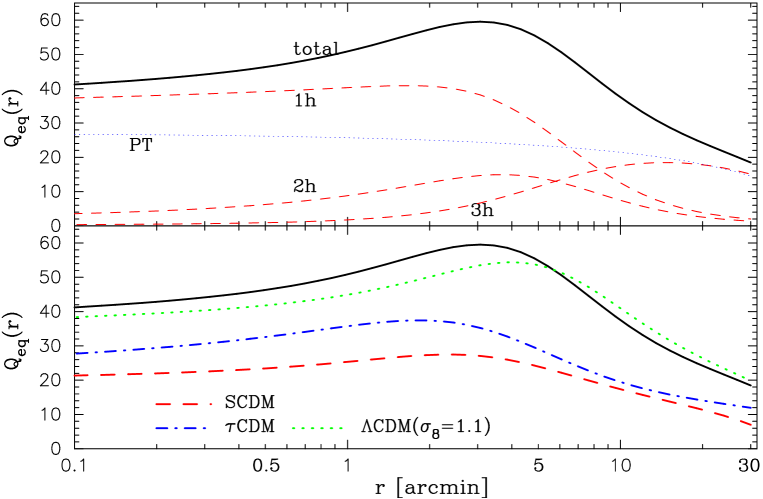
In Figure 22 we show $Q_{\kappa}$ for equilateral triangles as a function of side length. One can readily see that projection effects lead to greater contributions from the 2- and 3-halo terms, in contrast to the 3D case shown in Figure 7. One caveat that should be noted, as discussed for Figure 7 and 8, is that the halo model might overestimate $Q$ at the transition scale between the quasi-linear and non-linear regimes. This would be reflected in $Q_{\kappa}$ over the angular scales $0.1^{\prime}\lower 2.15277pt\hbox{$\;\buildrel<\over{\sim}\;$}r\lower 2.15277pt\hbox{$\;\buildrel<\over{\sim}\;$}20^{\prime}$, where the 2-halo term is relevant. This uncertainty needs further investigation by comparison with ray-tracing simulation results. The figure also shows that, on very small scales $\lower 2.15277pt\hbox{$\;\buildrel<\over{\sim}\;$}1^{\prime}$, the 1-halo term of $Q$ decreases slightly with decreasing angular scale. The small scale slope of the 1-halo term is determined by the combined effects of the NFW profile, the mass function and the halo concentration in the halo model calculation. For lensing, the small scale slope of the 2PCF and 3PCF is not transparent due to projection effects.

In the lower panel of Figure 22, we plot $Q_{\kappa}$ for different cosmological models as shown in Figure 9. $Q_{\kappa}$ is sensitive to cosmological parameters, in particular to $\Omega_{\rm m0}$ parameter, in analogy with the sensitivity of the skewness parameters of weak lensing to $\Omega_{\rm m0}$ (see e.g. Bernardeau et al. 2003; TJ02). Hence, it is expected that measuring $Q_{\kappa}$ can be used to break the degeneracies in the determinations $\Omega_{\rm m0}$ and $\sigma_{8}$ so far from measurements of the shear 2PCF (e.g., Van Waerbeke et al. 2001).

4.4 Performance of our approximation for calculating the 1-halo term of the 3PCF

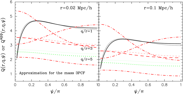
In Appendix B we present a useful approximation for calculating the one halo contribution to the mass 3PCF, which uses the Fourier-space halo model combined with the approximation developed in TJ02 for calculating the skewness and kurtosis parameters. Figure 23 demonstrates the performance of our approximation by comparing the results with the exact values computed from the real-space halo model. We have used the approximation for the 3PCF calculation in the numerator of $Q$, and the 2PCF calculation in the denominator includes full contributions from the 1- and 2-halo terms. We consider some of the triangle shapes shown in Figure 5. The left and right panels show the results for $r=0.02$ and $0.1~{}h^{-1}{\rm Mpc}$. In each panel, the solid, dashed and dotted curves are for $q/r=1$, $3$ and $5$, respectively. Note that all the triangles considered are in the strongly non-linear regime since we wish to check the validity of our approximation for the 1-halo term. The thin curves are the exact predictions from the real-space halo model computed from equation (44), while the thick curves denote the results of the approximation (72). The comparison demonstrates that the approximation works remarkably well with an accuracy of $\lower 2.15277pt\hbox{$\;\buildrel<\over{\sim}\;$}5\%$ for $q/r=1$ and $3$, and $\lower 2.15277pt\hbox{$\;\buildrel<\over{\sim}\;$}10\%$ even for elongated triangles with $q/r=5$. The three dot-dashed curves show the results of each term in the approximation (72) for $q/r=3$. Interestingly, although each term does not work well, the approximation obtained by summing them is close to the exact value. We have confirmed that the approximation of equation (73) for the 1-halo term of the weak lensing 3PCF also works to about the same accuracy as the 3D case shown here.

Figure 23: The performance of our approximation (72) for calculating the 1-halo contribution to the mass 3PCF. The results are shown for the triangle configurations as in Figure 5. We consider the non-linear scales $r=0.02$ (left panel) and $0.1~{}h^{-1}$Mpc (right). The thin curves are the exact halo model predictions, while the thick curves show the results of the approximation of equation (72). The three dot-dashed curves show each term in the approximation (72) for $q/r=3$. This figure verifies that our approximation accurately describes the 3PCF, even though each term in equation (72) is far from the exact value.

5 Discussion and Conclusion

In this paper, we have used the halo clustering model to compute the 3-point correlation function (3PCF) of cosmological fields. We have shown results for the three-dimensional mass and galaxy distributions and the two-dimensional weak lensing convergence field. The halo model enables us to separately consider the contributions to the 3PCF arising from triplets in a single halo or two or three different halos. Thus we can understand how gravitational clustering transitions from the quasi-linear regime to the strongly non-linear regime as one goes to smaller scales. We found that the single halo contribution, which is dominant on small scales, can be computed using the real-space formulation of the halo model far more easily than the Fourier-space approach used in the literature. We also developed approximations for computing the 2- and 3-halo contributions to the 3PCF. Since measuring the real space 3PCF on small scales is likely to be easier than the bispectrum, our model predictions will allow for the extraction of cosmological information from forthcoming galaxy surveys and weak lensing surveys.

We obtained the following results by applying our halo model to the concordance CDM model ($\Lambda$CDM). The 3PCF on small scales $r\lower 2.15277pt\hbox{$\;\buildrel<\over{\sim}\;$}1~{}h^{-1}{\rm Mpc}$ is dominated by the 1-halo term. Hence it probes properties of massive halos and can be used to constrain halo profiles as discussed below. The quasi-linear 3PCF predicted by perturbation theory can be reproduced by the 3-halo contribution for $r\lower 2.15277pt\hbox{$\;\buildrel>\over{\sim}\;$}3~{}h^{-1}$Mpc. For plausible halo model parameters, the hierarchical ansatz for the reduced 3PCF parameter, $Q={\rm constant}$, does not hold over the range of scales we have considered. However the $Q$ parameter does have a weaker dependence on triangle configurations in the non-linear regime than in the quasi-linear regime (see Figures 5 and 10). These results qualitatively verify the results in Ma & Fry (2000b,c). Ma & Fry also pointed out that the halo model for plausible model parameters violates the stable clustering hypothesis which has been widely used to develop analytical prediction of the non-linear gravitational clustering, as done in the popular PD fitting formula. In fact, very recently Smith et al. (2002) showed a weak violation of the stable clustering hypothesis using high-resolution $N$-body simulations. However, our halo model predictions for the 3PCF do not match the asymptotic shape proposed in Ma & Fry (2000b) because of the assumptions employed in the asymptotic formula. Therefore, it it merits further study to carefully investigate how small-scale gravitational clustering can be described by the halo model ingredients. Such a study can be carried out with the halo model methods developed in this paper.

We also found that the non-linear 3PCF is most sensitive to the inner slope of the halo profile and to the halo concentration parameter for given cosmological parameters (see Figures 12, 13 and 14). Combinations of the inner slope and the concentration can be adjusted so that the halo model matches the 2PCF result (see Figure 2). However only one combination can match both the 2- and 3PCFs. Hence in combination with the 2PCF, the non-linear 3PCF could be used to constrain the properties of dark matter halos. We suggest that the use of higher order correlations is a useful way of measuring the properties of massive halos. For example, while lensing surveys of clusters can be used to measure cluster halo profiles directly, this involves identifying cluster centers and assigning masses to clusters to measure averaged profiles. In contrast, by measuring the 2- and 3PCFs, parameters of the halo mass function and profile can be fitted for. While this approach is more challenging computationally, and requires some theoretical assumptions, it treats the data more objectively.

Our halo model predictions match the simulation results of Jing & Börner (1998) in the non-linear regime as well as the quasi-linear regime, as shown in Figure 10. However, the halo model seems to be less accurate on the intermediate transition scale $\sim 1~{}h^{-1}{\rm Mpc}$. Figure 7 shows that the predicted $Q$ parameter for equilateral triangles has a bump at this scale, which corresponds to the bump found for the reduced bispectrum at $k\sim 1~{}h\ {\rm Mpc}^{-1}$ by Scoccimarro et al. (2001). This is unlikely to reflect real properties of dark matter clustering. Rather, we argued that the bump feature is sensitive to the sharp cutoff of halos at the virial radius and the exclusion effect for the 2- and 3-halo terms. We explored alternative prescriptions as shown in Figure 8. To resolve this, detailed calculations and comparisons of the halo model predictions with simulation results will be needed.

We extended the halo model to predict the 3PCF of the galaxy distribution. Once we model how galaxies populate a halo of given mass, the halo occupation number, we can straightforwardly predict the galaxy 3PCF based on the halo model developed here. For the halo occupation number for red galaxies we have used, the galaxy 3PCF has a smaller amplitude and weaker dependence on triangle configuration compared to the mass 3PCF (Figures 17 and 18). This trend is indeed consistent with the actual measurements in Jing & Börner (1998). On the other hand, the 3PCF of blue galaxies displays complex features reflecting the input model of the halo occupation number. Thus, the galaxy 3PCF can be used to constrain the galaxy formation scenario as a function of host halo properties and galaxy type. Further work is needed to model the expected properties of galaxies by type for specific surveys and compute the resulting 3PCF.

As an example of the angular 3PCF, we have computed the 3PCF of the weak lensing convergence field. In particular, we employed the real-space halo model to compute the single halo contribution, as for the 3D case, which enabled us to compute the 1-halo term by a 4-dimensional integration. We verified that the real-space halo model is equivalent to the Fourier-space model well studied in the literature (see Figure 3). We also developed approximations for calculating the 2- and 3-halo terms. Because of projection effects, the 2- and 3-halo terms contribute to the 3PCF over a wider range of scales for the angular 3PCF compared to the 3D 3PCF. The resulting 3PCF does not obey the hierarchical ansatz over the angular scales we have considered. The lensing 3PCF is sensitive to cosmological parameters, in particular $\Omega_{\rm m0}$. Comparing measurements with model predictions of the 3PCF can be a useful tool to break degeneracies between the power spectrum and $\Omega_{\rm m0}$. We intend to compute 3-point functions of the shear field following Schneider & Lombardi (2002) and Zaldarriaga & Scoccimarro (2002) as these are easier to measure from the data. In Takada & Jain (2003), we presented a brief investigation of the 3PCFs of shear fields, where we found good agreement between the halo model prediction and the results measured from the ray-tracing simulations. It is also expected that the $n$-point correlations of weak lensing on sub-arcminute scales contain a wealth of information on properties of massive halos, beyond their dependence on cosmological parameters. The real-space halo model we have developed will be a useful analytical tool for such calculations.

The halo model presented in this paper allows for several interesting applications. First, the model can be extended to investigate the effect of triaxial halo shapes on the 3PCF, since it is the lowest-order statistical probe of non-sphericity. So far halo model applications assume a single, spherically symmetric profile. Recently, based on high-resolution simulations, Jing & Suto (2002) showed that halos are more accurately described by triaxial halo profiles than the spherically symmetric NFW profile. They claimed that the axis ratios typically have vales of $\sim 0.6$ for the smallest and largest axis. The non-sphericity of the halo profile could lead to a characteristic configuration dependence of the 3PCF. This effect should also affect the interpretation of cosmic shear measurements (Jing 2002). Likewise, the formulation developed in Sheth & Jain (2002) can be used to discuss the effects of substructure within halos on the 2PCF and 3PCF.

The real-space halo model can be directly used to compute the covariance of the 2PCF. As discussed in Cooray & Hu (2001b), the mass distribution on small scales displays pronounced non-Gaussian features induced by non-linear gravitational clustering. Hence one needs to take into account the non-Gaussian errors arising from the 4-point correlation function (4PCF). On the scales of interest the single halo contribution should dominate the error. The real-space halo model allows us to analytically compute the error contribution arising from the 4PCF with no additional computational effort than for the 3PCF (see §2.1).

In Appendix B, we constructed an approximation for calculating the 1-halo term of the 3PCF based on the Fourier-space halo model. We showed that the the approximation accurately describes the amplitude and configuration dependence of the 3PCF (see Figure 23). We will employ this approximation to perform an analytical study of the pairwise peculiar velocity dispersion (PVD) within the BBGKY hierarchy formalism (Peebles 1980). The PVD can be measured through the redshift distortions inferred from galaxy surveys (e.g., Zehavi et al. 2002). The BBGKY picture tells us that the PVD arises mainly from the 3PCF on small scales. However, there has been no comprehensive analytical model to describe the non-linear PVD. This is because of the complex form of the BBGKY hierarchy equations. Peebles (1980) (see Mo, Jing & Börner 1997; Jing et al. 1998 for a detailed study) assumed the hierarchical form for the non-linear 3PCF, although it turns out to be violated for CDM models. The isothermal assumption for the velocity distribution within a given halo was employed to analytically obtain the PVD based on the halo model (Sheth et al. 2001). It is important to clarify whether the BBGKY hierarchy leads to a self-consistent PVD for the CDM model. Moreover, we can easily combine the halo model prediction with models of the halo occupation number of galaxies to predict the PVD for different galaxy types, following the approach in §4.2.3.

We would like to thank R. Sheth, R. Scoccimarro, I. Szapudi, A. Taruya and L. Hui for several valuable discussions. We thank Y. P. Jing for kindly providing us with his simulation data results. Helpful comments from the referee, Chung-Pei Ma, led to improvements in the paper. This work is supported by NASA grants NAG5-10923, NAG5-10924 and a Keck foundation grant.

Appendix A Approximation for the 2- and 3-halo terms of the 3PCF

In this appendix, we present approximations used for the predictions of the 2- and 3-halo contributions to the 3PCF of the density field. The approximations are based on the Fourier-space halo model, combined with an approximation for the configuration dependence of the bispectrum from Scoccimarro et al. (2001; see also TJ02).

A.1 3D 3-point correlation function

Following the Fourier-space halo model, as discussed in §2.2, the 2-halo term for the mass 3PCF can be expressed from equations (11) and (13) as

$$\zeta_{2h}(\mbox{{\it\boldmath$r$}}_{1},\mbox{{\it\boldmath$r$}}_{2},\mbox{{\it\boldmath$r$}}_{3}) = \left[\int\!\!dmn(m)\left(\frac{m}{\bar{\rho}_{0}}\right)^{2}b(m)\int\!\!\frac{d^{3}\mbox{{\it\boldmath$k$}}_{1}}{(2\pi)^{3}}\tilde{u}_{m}(k_{1})\exp[i\mbox{{\it\boldmath$k$}}_{1}\cdot\mbox{{\it\boldmath$r$}}_{12}]\right]\tilde{u}_{m}(k_{12})$$ (61)

$$\times\left[\int\!\!dm^{\prime}~{}n(m^{\prime})\left(\frac{m^{\prime}}{\bar{\rho}_{0}}\right)b(m^{\prime})\int\!\!\frac{d^{3}\mbox{{\it\boldmath$k$}}_{2}}{(2\pi)^{3}}\tilde{u}_{m^{\prime}}(k_{2})P^{L}(k_{2})\exp[i\mbox{{\it\boldmath$k$}}_{2}\cdot\mbox{{\it\boldmath$r$}}_{32}]\right]+\mbox{\rm cyc.},$$

where the bias parameter $b(m)$ is given by equation (22). As discussed in Scoccimarro et al. (2001), the physical meaning of the 2-halo term tells us that the main contribution to the first term on the r.h.s arises from modes with $k_{1}\gg k_{2}$, leading to the approximation $k_{12}\approx k_{1}$. Replacing $\tilde{u}_{m}(k_{12})$ with $\tilde{u}_{m}(k_{1})$ allows us to perform analytically the angular integration in $\int d^{3}\mbox{{\it\boldmath$k$}}_{i}$ in the first term above. Using similar procedures for the second and third terms on the r.h.s. yields the following approximation:

$$\zeta^{\rm app}_{2h}(\mbox{{\it\boldmath$r$}}_{1},\mbox{{\it\boldmath$r$}}_{2},\mbox{{\it\boldmath$r$}}_{3}) = \left[\int\!\!dm~{}n(m)\left(\frac{m}{\bar{\rho}_{0}}\right)^{2}b(m)\int\!\!\frac{k_{1}^{2}dk_{1}}{2\pi^{2}}(\tilde{u}_{m}(k_{1}))^{2}j_{0}(k_{1}r_{12})\right]$$ (62)

$$\times\left[\int\!\!dm^{\prime}~{}n(m^{\prime})\left(\frac{m^{\prime}}{\bar{\rho}_{0}}\right)b(m^{\prime})\int\!\!\frac{k^{2}_{2}dk_{2}}{2\pi^{2}}\tilde{u}_{m^{\prime}}(k_{2})P^{L}(k_{2})j_{0}(k_{2}r_{23})\right]+\mbox{\rm cyc.}$$

where we have used the formula $\int\!\!d\Omega_{\mbox{{\it\boldmath$k$}}}\exp[i\mbox{{\it\boldmath$k$}}\cdot\mbox{{\it\boldmath$r$}}]=j_{0}(kr)$. The large square bracket is meant to show explicitly that the integrations inside each bracket can be done separately from the other. Thus one needs to perform only 2-dimensional integrations to get the 2-halo term. It was shown that a similar approximation for the skewness calculation turns out to be accurate (Scoccimarro et al. 2001; TJ02). Hence, we expect that this also holds for the 3PCF calculation.

The 3-halo contribution to the 3PCF can be expressed as

$$\zeta_{3h}(\mbox{{\it\boldmath$r$}}_{1},\mbox{{\it\boldmath$r$}}_{2},\mbox{{\it\boldmath$r$}}_{3}) = \int\!\!dm~{}n(m)\left(\frac{m}{\bar{\rho}_{0}}\right)b(m)\int\!\!dm^{\prime}~{}n(m^{\prime})\left(\frac{m}{\bar{\rho}_{0}}\right)b(m)\int\!\!dm^{\prime\prime}~{}n(m^{\prime\prime})\left(\frac{m^{\prime\prime}}{\bar{\rho}_{0}}\right)b(m^{\prime\prime})$$ (63)

$$\times\left[\int\!\!\frac{d^{3}\mbox{{\it\boldmath$k$}}_{1}}{(2\pi)^{3}}\frac{d^{3}\mbox{{\it\boldmath$k$}}_{2}}{(2\pi)^{3}}u_{m}(k_{1})u_{m^{\prime}}(k_{2})u_{m^{\prime\prime}}(k_{12})e^{i\mbox{{\it\boldmath$k$}}_{1}\cdot\mbox{{\it\boldmath$r$}}_{13}+i\mbox{{\it\boldmath$k$}}_{2}\cdot\mbox{{\it\boldmath$r$}}_{23}}P^{L}(k_{1})P^{L}(k_{2})\right.$$

$$\times\left.\left\{\frac{10}{7}+\left(\frac{1}{k_{1}^{2}}+\frac{1}{k_{2}^{2}}\right)\mbox{{\it\boldmath$k$}}_{1}\cdot\mbox{{\it\boldmath$k$}}_{2}+\frac{4}{7}\frac{(\mbox{{\it\boldmath$k$}}_{1}\cdot\mbox{{\it\boldmath$k$}}_{2})^{2}}{k_{1}^{2}k_{2}^{2}}\right\}+\mbox{\rm cyc.}\right].$$

We again employ the approximation $\tilde{u}_{m^{\prime\prime}}(k_{12})\approx\tilde{u}_{m^{\prime\prime}}(k_{1})$ to perform analytically the integration for the first term on the r.h.s., although there is no guarantee that the approximation is as accurate as for the 2-halo term. Following the procedure developed to derive the perturbation theory 3PCF (Fry 1984b; also see Jing & Börner 1997; Gaztañaga & Bernardeau 1998; Barriga & Gaztañaga 2002) we can derive the approximation for the 3-halo term:

$$\zeta^{3h}_{\kappa}(\mbox{{\it\boldmath$r$}}_{1},\mbox{{\it\boldmath$r$}}_{2},\mbox{{\it\boldmath$r$}}_{3}) = \frac{10}{7}\Xi^{(2)}(r_{13})\Xi^{(1)}(r_{23})-\frac{4}{7}\left(-3\frac{\Phi^{(2)\prime}(r_{13})}{r_{13}}\frac{\Phi^{(1)\prime}(r_{23})}{r_{23}}-\frac{\Xi^{(2)}(r_{13})\Phi^{(1)\prime}(r_{23})}{r_{23}}-\frac{\Xi^{(1)}(r_{23})\Phi^{(2)\prime}(r_{13})}{r_{13}}\right)$$ (64)

$$-\mu_{1323}\left(\Xi^{(2)\prime}(r_{13})\Phi^{(1)\prime}(r_{23})+\Xi^{(1)\prime}(r_{23})\Phi^{(2)\prime}(r_{13})\right)$$

$$+\frac{4}{7}\mu_{1323}^{2}\left(\Xi^{(2)}(r_{13})+3\frac{\Phi^{(2)\prime}(r_{13})}{r_{13}}\right)\left(\Xi^{(1)}(r_{23})+3\frac{\Phi^{(1)\prime}(r_{23})}{r_{23}}\right)+{\rm cyc.},$$

where $\mu_{1323}\equiv(\mbox{{\it\boldmath$r$}}_{13}\cdot\mbox{{\it\boldmath$r$}}_{23})/(r_{13}r_{23})$ and

$$\Xi^{(\mu)}(r) \equiv \int\!\!\frac{k^{2}dk}{2\pi^{2}}\left[\int\!\!dm~{}n(m)\left(\frac{m}{\bar{\rho}_{0}}\right)b(m)u_{m}(k)\right]^{\mu}P^{L}(k)\frac{\sin(kr)}{kr},$$

$$\Phi^{(\mu)}(r) \equiv \int\!\!\frac{k^{2}dk}{2\pi^{2}}\left[\int\!\!dm~{}n(m)\left(\frac{m}{\bar{\rho}_{0}}\right)b(m)u_{m}(k)\right]^{\mu}\frac{P^{L}(k)}{k^{2}}\frac{\sin(kr)}{kr}.$$

We find that this approximation reproduces the perturbation theory result at scales $\lower 2.15277pt\hbox{$\;\buildrel>\over{\sim}\;$}5~{}h^{-1}$Mpc for the $\Lambda$CDM model (see Figure 7). Note that, for the actual predictions of the 3PCF shown in this paper, we have used the permutation $(1)\leftrightarrow(2)$ for terms such as $\Xi^{(2)}\Xi^{(1)}$ in the above equation, so that it satisfies statistical symmetry for permutations between $\mbox{{\it\boldmath$r$}}_{1}$, $\mbox{{\it\boldmath$r$}}_{2}$ and $\mbox{{\it\boldmath$r$}}_{3}$.

By replacing $(m/\bar{\rho}_{0})$ in equations (62) and (64) with the halo occupation number of galaxies $\langle{N_{\rm gal}}\rangle(m)/\bar{n}_{\rm gal}$, as discussed in §4.2.3, we obtain the corresponding approximations for computing the 2- and 3-halo contributions to the 3PCF of galaxies.

A.2 2D 3-point correlation function

It is straightforward to extend the approximations for the 3-dimensional 3PCF to the 3PCF of weak lensing fields. As discussed for equation (41), combining equation (62) with Limber’s equation yields the following approximation for the 2-halo term of the weak lensing convergence:

$$Z^{\rm app}_{2h}(\mbox{{\it\boldmath$r$}}_{1},\mbox{{\it\boldmath$r$}}_{2},\mbox{{\it\boldmath$r$}}_{3}) = \int^{\chi_{s}}_{0}\!\!d\chi W^{3}(\chi,\chi_{s})d_{A}^{-4}\left[\int\!\!dm~{}n(m)\left(\frac{m}{\bar{\rho}_{0}}\right)^{2}b(m)\int\!\!\frac{l_{1}dl_{1}}{2\pi}(\tilde{u}_{m}(k_{1}))^{2}J_{0}(l_{1}r_{12})\right.$$ (66)

$$\times\left.\int\!\!dm^{\prime}~{}n(m^{\prime})\left(\frac{m^{\prime}}{\bar{\rho}_{0}}\right)b(m^{\prime})\int\!\!\frac{l_{2}dl_{2}}{2\pi}\tilde{u}_{m^{\prime}}(k_{2})P^{L}(k_{2};\chi)J_{0}(l_{2}r_{23})+\mbox{\rm cyc.}\right],$$

where $k_{i}=l_{i}/d_{A}(\chi)$. Note that the redshift dependence of $P^{L}(k;\chi)$ is given by the linear growth factor $D(z)$.

Likewise, the approximation for the 3-halo term can be obtained by the following replacements in equation (64) and the additional integration over the redshift:

$$(\Xi,\Phi\rightarrow\Xi_{2D},\Phi_{2D})\mbox{ in }\zeta^{\rm app}_{3h},$$ (67)

where $\mu_{1323}\equiv(\mbox{{\it\boldmath$r$}}_{13}\cdot\mbox{{\it\boldmath$r$}}_{23})/(r_{13}r_{23})$ and

$$\Xi^{(\mu)}_{2D}(r) \equiv \int\!\!\frac{ldl}{2\pi}\left[\int\!\!dm~{}n(m)\left(\frac{m}{\bar{\rho}_{0}}\right)b(m)u_{m}(k)\right]^{\mu}P^{L}(k)J_{0}(lr),$$

$$\Phi^{(\mu)}_{2D}(r) \equiv \int\!\!\frac{k^{2}dk}{2\pi^{2}}\left[\int\!\!dm~{}n(m)\left(\frac{m}{\bar{\rho}_{0}}\right)b(m)u_{m}(k)\right]^{\mu}\frac{P^{L}(k)}{k^{2}}J_{0}(lr).$$ (68)

Appendix B Approximations for the 1-halo term of the 3PCF

In this section, we present approximations for calculating the 1-halo contribution to the 3D or 2D 3PCF with the Fourier-space halo model. These are combined with the approximation in TJ02 for calculating the skewness parameter of the density field.

B.1 3D 3-point correlation function

Based on the Fourier-space halo approach, the 1-halo contribution to the 3PCF of the density field can be obtained from equations (11) and (6) as

$$\zeta_{1h}(\mbox{{\it\boldmath$r$}}_{1},\mbox{{\it\boldmath$r$}}_{2},\mbox{{\it\boldmath$r$}}_{3})=\int\!\!dm~{}n(m)\left(\frac{m}{\bar{\rho}_{0}}\right)^{3}\int\!\!\prod_{i=1}^{3}\frac{d^{3}\mbox{{\it\boldmath$k$}}_{i}}{(2\pi)^{3}}\tilde{u}_{m}(\mbox{{\it\boldmath$k$}}_{i})\exp[i\mbox{{\it\boldmath$k$}}_{i}\cdot\mbox{{\it\boldmath$r$}}_{i}](2\pi)^{3}\delta_{D}(\mbox{{\it\boldmath$k$}}_{123}).$$ (69)

The Dirac-delta function allows us to eliminate one of the three wavevectors $\mbox{{\it\boldmath$k$}}_{i}$. For example, let us eliminate $\mbox{{\it\boldmath$k$}}_{3}$, leading to the replacement $\mbox{{\it\boldmath$k$}}_{3}=-\mbox{{\it\boldmath$k$}}_{12}$ in the above equation. Then, the integrand has dependences on $d^{3}\mbox{{\it\boldmath$k$}}_{i}$ via $\tilde{u}_{m}(k_{12})$ and $\exp[i\mbox{{\it\boldmath$k$}}_{i}\cdot\mbox{{\it\boldmath$r$}}_{i}]$. TJ02 proposed that the angular dependence of $\tilde{u}_{m}(k_{12})$ can be approximated with the replacement:

$$\tilde{u}_{m}(k_{12})\longrightarrow\tilde{u}_{m}(\tilde{k}_{12}),$$ (70)

where $\tilde{k}_{12}=(k_{1}^{2}+k_{2}^{2}-k_{1}k_{2})^{1/2}$. TJ02 showed that this replacement works well for predictions of the skewness parameters of the 3D density field and the weak lensing field. If we assume that this holds for the 3PCF calculation, we can analytically perform the angular integrations in $\int\,d^{3}\mbox{{\it\boldmath$k$}}_{i}$, to get

$$\zeta_{1h}(\mbox{{\it\boldmath$r$}}_{1},\mbox{{\it\boldmath$r$}}_{2},\mbox{{\it\boldmath$r$}}_{3})\approx F_{\zeta}(r_{13},r_{23})\equiv\int\!\!dm~{}n(m)\left(\frac{m}{\bar{\rho}_{0}}\right)^{3}\int\!\!\frac{dk_{1}}{2\pi^{2}}\frac{dk_{2}}{2\pi^{2}}~{}k_{1}^{2}k_{2}^{2}\tilde{u}_{m}(k_{1})\tilde{u}_{m}(k_{2})\tilde{u}_{m}(\tilde{k}_{12})j_{0}(k_{1}r_{13})j_{0}(k_{2}r_{23}).$$ (71)

The above approximation reduces the 7-dimensional integral in equation (69) to a 3-dimensional one. However, the resulting 3PCF depends only on the two side lengths $r_{13}$ and $r_{23}$, and thus has no dependence on the interior angles. If we had started by eliminating $\mbox{{\it\boldmath$k$}}_{2}$ or $\mbox{{\it\boldmath$k$}}_{1}$ in equation (69), the resulting 3PCF would have dependences only on the two side lengths $r_{12}$ and $r_{23}$ or $r_{12}$ and $r_{13}$, respectively. Thus, the approximate result for the 3PCF has different forms even for the same triangle shape. To resolve this, we propose the following symmetrized form as the approximation for calculating $\zeta_{1h}$:

$$\zeta_{1h}^{\rm app}(\mbox{{\it\boldmath$r$}}_{1},\mbox{{\it\boldmath$r$}}_{2},\mbox{{\it\boldmath$r$}}_{3})=\frac{1}{3}\left[F_{\zeta}(r_{12},r_{13})+F_{\zeta}(r_{12},r_{23})+F_{\zeta}(r_{13},r_{23})\right],$$ (72)

The dependences of this form on the three parameters of the triangle shape, $r_{12}$, $r_{23}$ and $r_{31}$, are like the hierarchical form $\zeta=Q[\xi(r_{12})\xi(r_{31})+\xi(r_{12})\xi(r_{23})+\xi(r_{13})\xi(r_{22})]$. The factor $1/3$ is simply chosen so that it agrees with the third-order moment given in TJ02 for the limit $r,q\rightarrow 0$. As shown in §4.4, the approximation (72) is accurate compared with the exact value computed from equation (6), even though each term on the r.h.s is far from the exact value (see Figure 23).

B.2 2D 3-point function

In the spirit of equation (72), the corresponding approximation for the projected 3PCF given by equation (40) can be constructed as:

$$Z^{\rm app}_{1h}(\mbox{{\it\boldmath$\theta$}}_{1},\mbox{{\it\boldmath$\theta$}}_{2},\mbox{{\it\boldmath$\theta$}}_{3})=\frac{1}{3}\left[F_{Z}(\theta_{12},\theta_{13})+F_{Z}(\theta_{21},\theta_{23})+F_{Z}(\theta_{31},\theta_{32})\right],$$ (73)

with

$$F_{Z}(\theta,\varphi)\equiv\int^{\chi_{s}}_{0}\!\!d\chi~{}W^{3}(\chi)d_{A}^{-4}(\chi)\int\!\!dm~{}n(m)\left(\frac{m}{\bar{\rho}_{0}}\right)^{3}\int\frac{l_{1}dl_{1}}{2\pi}\frac{l_{2}dl_{2}}{2\pi}~{}\tilde{u}_{m}(k_{1})\tilde{u}_{m}(k_{2})\tilde{u}_{m}(\tilde{k}_{12})J_{0}(\theta l_{1})J_{0}(\varphi l_{2}),$$ (74)

where $k_{i}=l_{i}/d_{A}(\chi)$. The 4-dimensional integration required to carry out the above approximation is the same level of complexity as the real-space halo model expression in equation (40).

References

- [Bardeen et al. 1986] Bardeen, J. M., Bond, J. R., Kaiser, N., Szalay, A. S., 1986, ApJ, 304, 15
- [Barriga & Gaztañaga 2002] Barriga, J., Gaztañaga, E., 2002, MNRAS, 333, 443
- [Bartelmann 1996] Bartelmann, M., 1996, A&A, 313, 697
- [Bartelmann & Schneider 2001] Bartelmann, M., Schneider, P., 2001, Phys. Rep., 340, 291
- [Berlind & Weinberg 2002] Berlind, A. B., Weinberg, D. H., 2002, ApJ, 575, 587
- [Bernardeau et al. 2002b] Bernardeau, F., Colombi, S., Gaztañaga, E., Scoccimarro, R., 2002a, Phys. Rep., 367, 1
- [Bernardeau et al. 2002b] Bernardeau, F., Mellier, Y., Van Waerbeke, L., 2002b, A&A, 389, L28
- [Bernardeau, Van Waerbeke & Mellier 2003] Bernardeau, F., Van Waerbeke, L., Mellier, Y., 2003, A&A, 397, 405
- [Bond et al. 2002] Bond, J. R., et al., 2002, astro-ph/0205386
- [Bullock et al. 2001] Bullock, J. S., Kolatt, T. S., Sigad, Y., Somerville, R. S., Kravtsov, A. V., Klypin, A. A., Primack, J. R., Dekel, A., 2001, MNRAS, 321, 559
- [Cole & Kaiser 1988] Cole, S., Kaiser, N., 1988, MNRAS, 233, 637
- [Cooray 2002] Cooray, A., 2002, ApJ, 576, L105, astro-ph/0206388
- [Cooray & Hu 2001a] Cooray, A., Hu, W., 2001a, ApJ, 548, 7
- [Cooray & Hu 2001b] Cooray, A., Hu, W., 2001b, ApJ, 554, 56
- [Cooray & Sheth 2002] Cooray, A., Sheth, R., 2002, Physics Reports, 372, 1, astro-ph/0206508
- [Cooray et al. 2000] Cooray, A., Hu, W., Miralda-Escude, J., 2000, ApJ, 535, L9
- [de Bernardis et al. 2000] de Bernardis, et al., 2000, Nature, 404, 955
- [Eke, Cole & Frenk 1996] Eke, V. R., Cole, S., Frenk, C. S., 1996, MNRAS, 282, 263
- [Feldmann et al. 2001] Feldmann, H. A., Frieman, J. A., Fry, J. N., Scoccimarro, R., 2001, PRL, 86, 1434
- [Frieman & Gaztañaga 1999] Frieman, J. A., Gaztañaga, E., 1999, ApJ, 421, L83
- [Gaztaaga & Bernardeau 1998] Gaztaaga, E., Bernardeau, F., 1998, A&A, 331, 829
- [Gradshteyn & Ryzhik 2000] Gradshteyn, L. S., Ryzhik, I. M., 2000, Tabel of Integrals, Series, and Products, (6th ed.; San Diego, Academic Press)
- [Fry 1984a] Fry, J. N., 1984a, ApJ, 277, L5
- [Fry 1984b] Fry, J. N., 1984b, ApJ, 279, 499
- [Fukushige & Makino 1997] Fukushige, T., Makino, J., 1997, ApJ, 477, L9
- [Groth & Peebles 1977] Groth, E. J., Peebles, P. J. E., 1977, ApJ, 217, 385
- [Hamana, Yoshida & Suto 2002] Hamana, T., Yoshida, N., Suto, Y., 2002, ApJ, 568, 455
- [Hamilton 1988] Hamilton, A. J. S., 1988, ApJ, 332, 67
- [Hamilton & Tegmark 2002] Hamilton, A. J. S., Tegmark, M., 2002, MNRAS, 330, 506
- [Hamilton et al. 1991] Hamiltion, A. J. S., Matthews, A., Kumar, P., Lu, E., 1991, ApJ, 374, L1
- [Henry 2000] Henry, J. P., 2000, ApJ, 534, 565
- [Jain 1997] Jain, B., 1997, MNRAS, 287, 687
- [Jain & Bertschinger 1994] Jain, B., Bertschinger, E., 1994, ApJ, 431, 495
- [Jain & Seljak 1997] Jain, B., Seljak, U., 1997, ApJ, 484, 560
- [Jain, Mo & White 1995] Jain, B., Mo, H. J., White, S. D. M., 1995, MNRAS, 276, L25
- [Jing 1998] Jing, Y. P., 1998, ApJ, 503, L9
- [Jing 2002] Jing, Y. P., 2002, MNRAS, 335, L89, astro-ph/020609
- [Jing & Börner 1997] Jing, Y. P., Börner, G., 1997, A&A, 318, 667
- [Jing & Börner 1998] Jing, Y. P., Börner, G., 1998, ApJ, 503, 37
- [Jing & Suto 2000] Jing, Y. P., Suto, Y., 2000, ApJ, 529, L69
- [Jing & Suto 2002] Jing, Y. P., Suto, Y., 2002, ApJ, 574, 538, astro-ph/0204108
- [Jing Mo & Börner 1998] Jing, Y. P., Mo, H., Börner, G., 1998, ApJ, 494, 1
- [Kaiser 1992] Kaiser, N., 1992, ApJ, 388, 272
- [Kauffmann et al. 1999] Kauffmann, G., Colberg, J. M., Diaferio, A., & White, S. D. M., 1999, MNRAS, 303, 188
- [Limber 1954] Limber, D., 1954, ApJ, 119, 655
- [Ma & Fry 2000a] Ma, C.-P. Fry, J. N., 2000a, ApJ, 531, L87
- [Ma & Fry 2000b] Ma, C.-P. Fry, J. N., 2000b, ApJ, 538, L107
- [Ma & Fry 2000c] Ma, C.-P. Fry, J. N., 2000c, ApJ, 543, 503
- [Matsubara & Suto 1994] Matsubara, T., Suto, Y., 1994, ApJ, 420
- [McClelland & Silk 1977] McClelland, J., Silk, J., 1977, ApJ, 217, 331
- [Mo & White 1996] Mo, H. J., White, S. D. M., 1996, MNRAS, 282, 347
- [Mo, Jing & Börner 1997] Mo, H. J., Jing, Y. P., Börner, G., 1997, MNRAS, 286, 979
- [Mo, Jing & White 1997] Mo, H. J., Jing, Y. P., White, S. D. M., 1997, MNRAS, 290, 651
- [Moore et al. 1998] Moore, B., Governato, F., Quinn, T., Stadel, J., Lake G., 1998, ApJ, 499, L5
- [Moustakas & Somerville 2002] Moustakas, L. A., Somerville, R. S., 2002, ApJ, 577, 1
- [Nakamura & Suto 1997] Nakamura, T. T., Suto, Y., 1997, Prog. Theor. Phys., 97, 49
- [Navarro, Frenk & White 1997] Navarro, J., Frenk, C., White, S. D. M., 1997, ApJ, 490, 493 (NFW)
- [Neyman & Scott 1952] Neyman, J., & Scott, E. L., 1952, ApJ, 116, 144
- [Peacock & Doods 1996] Peacock, J. A., Dodds, S. J., 1996, MNRAS, 280, L19
- [Peacock & Smith 2000] Peacock, J. A., Smith, R. E., 2000, MNRAS, 318, 1144
- [Peebles 1974] Peebles, P. J. E., 1974, A&A, 32, 197
- [Peebles 1980] Peebles, P. J. E., 1980, Large-Scale Structure of the Universe (Princeton: Princeton Univ. Press)
- [Peebles & Groth 1975] Peebles, P. J. E., Groth, E. J., 1975, ApJ, 196, 1
- [Press & Schechter 1974] Press, W., Schechter, P., 1974, ApJ, 187, 425
- [Scherrer & Bertschinger 1991] Scherrer, R. J., Bertschinger, E., 1991, ApJ, 381, 349
- [Schneider & Lombardi 2002] Schneider, P., Lombardi, M., 2002, astro-ph/0207454
- [Schneider, Van Waerbeke & Mellier 2002] Schneider, P., Van Waerbeke, L., Mellier, Y., 2002, A&A, 389, 729
- [Scoccimarro & Friemann 1999] Scoccimarro, R., Friemann, J., 1999, ApJ, 520, 35
- [Scoccimarro et al. 2001] Scoccimarro, R., Sheth, R. K., Hui, L., Jain, B., 2001, ApJ, 546, 652
- [Scranton 2002] Scranton, R., 2002, astro-ph/0205517
- [Seljak 2000] Seljak, U., 2000, MNRAS, 318, 203
- [Sheth & Jain 1997] Sheth, R. K., Jain, B., 1997, MNRAS, 285, 231
- [Sheth & Jain 2002] Sheth, R. K., Jain, B., 2002, submitted to MNRAS, astro-ph/0208353
- [Sheth & Lemson 1999] Sheth, R. K., Lemson, G., 1999, MNRAS, 304, 767
- [Sheth & Tormen 1999] Sheth, R. K., Tormen, G., 1999, MNRAS, 308, 119
- [Sheth et al. 2001] Sheth, R. K., Diaferio, A., Hui, L., Scoccimarro, R., 2001, MNRAS, 326, 463
- [Smith et al. 2002] Smith, R. E., Peacock, J. A., Jenkins, A., White, S. D. M., Frenk, C. S., Pearce, F. R., Thomas, P. A., Efstathiou, G., Couchman, H. M., P., 2002, astro-ph/0207664 (Smith02)
- [Suto & Matsubara 1994] Suto, Y., Matsubara, T., 1994, ApJ, 504
- [Szapudi et al. 1999] Szapudi, I., Quinn, T., Stadel, J., Lake, G., 1999, ApJ, 517, 54
- [Taruya, Hamana & Kayo 2002] Taruya, A., Hamana, T., Kayo, I., 2002, MNRAS in press, astro-ph/0210507
- [Takada & Jain 2002a] Takada, M., Jain, B., 2002a, MNRAS, 337, 875, astro-ph/0205055, (TJ02)
- [Takada & Jain 2003] Takada, M., Jain, B., 2003, ApJ, 583, L49, astro-ph/0210261
- [Totsuji69] Totsuji, H., Kihara, T., 1969, PASJ, 21, 221
- [Verde et al. 2001] Verde, L., et al., 2002, MNRAS , 335, 432
- [Van Waerbeke et al. 2001] Van Waerbeke, L. et al., 2001, A&A, 374, 757
- [Wright & Brainerd 2000] Wright, C. O., Brainerd, T. G., 2000, ApJ, 534, 34
- [Yano & Gouda 1999] Yano, T., Gouda, N., 1999, ApJ, 539, 493
- [Zaldarriaga & Scoccimarro 2002] Zaldarriaga, M., Scoccimarro, R., 2002, astro-ph/0208075
- [Zehavi et al. 2002] Zehavi, I., et al., 2002, ApJ, 571, 172