Factors Determining Variability Time in Active Galactic Nucleus Jets

Abstract

The relationship between observed variability time and emission region geometry is explored for the case of emission by relativistic jets. The approximate formula for the jet-frame size of the emission region, $R^{\prime}=Dc\Delta t_{\rm obs}$ is shown to lead to large systematic errors when used together with observed luminosity and assumed or estimated Doppler factor $D$ to estimate the jet-frame photon energy density. These results have implications for AGN models in which low-energy photons are targets for interaction of high energy particles and photons, e.g. synchrotron-self Compton models and hadronic blazar models, as well as models of intra-day variable sources in which the photon energy density imposes a brightness temperature limit through Compton scattering.

The actual relationship between emission region geometry and observed variability is discussed for a variety of geometries including cylinders, spheroids, bent, helical and conical jet structures, and intrinsic variability models including shock excitation. The effects of time delays due to finite particle acceleration and radiation time scales are also discussed.

¹Department of Physics and Mathematical Physics, The University of Adelaide, Adelaide, SA 5005, Australia
rprother@physics.adelaide.edu.au

Keywords: active galactic nuclei, blazars, variability, emission region

1 Introduction

In the standard picture of active galactic nuclei (AGN), accretion onto a super-massive black hole is via an accretion disk, and a significant fraction of the accretion power (possibly supplemented by tapping into the rotational energy of the black hole) produces twin opposing relativistic jets moving outward along the disk axis, with typical Lorentz factors $\Gamma\sim 2$–10 as inferred from very long baseline interferometry (VLBI) observations. The objects observed in high energy $\gamma$ rays are “blazars”, AGN in which one of the jets is closely aligned toward the observer. It is natural that in $\gamma$-rays we should see preferentially those AGN with aligned jets because the emission from the jet is Doppler boosted in energy and relativistically beamed along the jet direction (for a discussion of relativistic effects see Urry and Padovani 1995). The $\gamma$ ray emission from blazars is variable (as it is also at optical, UV and X-ray energies). Relativistic effects also cause the observed variability time to be shorter than the time scale over which the emission changes in the jet frame.

The spectral energy distribution (SED) of blazars shows two broad peaks, the low energy peak extending from the infrared to the UV or X-ray region of the spectrum, and the high energy peak starting in the X-ray or $\gamma$ ray range. The usual interpretation is that relativistic electrons produce the low energy part by synchrotron emission, and that the same electrons produce the high energy part by Compton scattering the low energy part and/or external photons to higher energies. The 3rd EGRET catalog of high-energy $\gamma$-ray sources (Hartman et al. 1999) contains around 70 high confidence identifications of AGN, and all appear to be blazars (Montigny et al. 1995, Mukherjee et al. 1997). Clearly, the $\gamma$-ray emission is associated with AGN jets.

Four BL Lac objects have been detected in the TeV energy range: Mrk 421 (Punch et al. 1992), Mrk 501 (Quinn et al. 1996), 1E S2344+514 (Catanese et al. 1998) and PKS 2155-304 (Chadwick et al. 1999). Recently, the spectrum of Mrk 501 has been measured up to 24 TeV by the HEGRA telescopes (Konopelko et al. 1999). Several of the EGRET AGN show $\gamma$-ray variability with time scales of $\sim 1$ day (Kniffen et al. 1993) at GeV energies. The TeV $\gamma$-ray emission of two BL Lacs shows very rapid variability. For Mrk 421, variability on a time scale as short as $\sim 15$ minutes has been reported (Gaidos et al. 1996). In the case of Mrk 501, variability on a time scale of a few hours was observed during the 1997 high level of activity, and there is evidence of a 23 day periodicity (Protheroe et al. 1998, Hayashida et al. 1998) interpreted in terms of a binary black hole model for the central engine by Rieger and Mannheim (2000). These variability timescales place important constraints on the models. For example, the synchrotron self-Compton (SSC) model appears to be just consistent with recent multi-wavelength observations of Mrk 421 and Mrk 501 during flaring activity (Bednarek and Protheroe 1997, 1999). However, the allowed range of physical parameters (Doppler factor and magnetic field) is rather small, and this mechanism may well be excluded by future observations. For a recent review of TeV $\gamma$-ray astronomy see Kifune (2002).

Rapid variability in intra-day variability (IDV) sources is a long-standing problem as it implies apparent brightness temperatures in the radio regime which may exceed 10¹⁷ K or relativistic beaming with extremely high Doppler factors, coherent radiation mechanisms, or special geometric effects (Wagner and Witzel 1995). The very rapid flaring observed at TeV and X–ray energies during flaring activity in blazars also presents a challenge for any model and suggests a re-examination of mechanisms which may cause very rapid variability would be worthwhile. In this paper I concentrate on how the observed variability time is related to the geometry and motion of the emission region, and thus to the photon energy density in the emission region. The blazar emission mechanisms to be discussed include: a shock excited emission region, bent jets, a shock propagating along a jet containing a helical structure and illuminating parts of the helix by enhanced interactions/emission of radiation such that the emission regions move along helical paths, and highly oblique conical shocks in the jet. Together with geometry-specific time delays and variable Doppler boosting associated with relativistic motion of the emission region along a curved trajectory, it may well be possible to explain the observed flaring activity and high brightness temperatures. Another possibility briefly discussed in the context of bent jets and conical shocks is that jets may be fueled on an irregular time scale.

The observed variability time $\Delta t_{\rm obs}$, and some assumed or estimated Doppler factor $D$ is often used to estimate the jet-frame source radius, $R^{\prime}\approx Dc\Delta t_{\rm obs}$. The jet-frame photon energy density is then usually assumed to be $U^{\prime}_{\rm phot}\approx L^{\prime}/4\pi{R^{\prime}}^{2}c$, where $L^{\prime}$ is the jet-frame bolometric luminosity given by $L^{\prime}=D^{-4}4\pi d_{L}^{2}F$, $F$ being the observed bolometric flux, and $d_{L}$ being the luminosity distance. However, this approach can lead to large systematic errors in the jet-frame photon energy density. This is important because the energy density of photons of the low energy part of the SED may determine the energy losses of electrons, and the rate of up-scattering to $\gamma$-ray energies in SSC models, and the rate of proton-photon collisions in hadronic models (see, e.g., Mannheim and Biermann 1989, Protheroe 1997, Mannheim et al. 2001, Mücke and Protheroe 2001, Mücke et al. 2002). If the emission region is optically thin, it may also have consequences for IDV sources as I will show that it is quite possible that the photon energy density responsible for the so-called Compton catastrophe may actually be lower than usually estimated. In the following sections I shall discuss how the variability time is related to the emission region geometry and intrinsic jet-frame variability, show how this can lead to large systematic errors in the jet-frame photon energy density, and discuss other scenarios which can lead to rapid variability and high fluxes.

2 Relationship between variability time and emission region geometry

I shall discuss first a relativistic jet pointing at angle $\theta$ with respect to the line of sight to the observer, in which the emission region is a cylinder of radius $r$ and jet-frame length $\ell^{\prime}$ moving along the jet with the jet’s Lorentz factor $\Gamma=1/\sqrt{1-\beta^{2}}$. To work out how the observed lightcurve depends on the emission region geometry and the duration of the emission in the jet frame (primed coordinates) we first consider in the observer frame (unprimed coordinates) the events corresponding to: (i) the emission from centre of cylinder at $(t\equiv t_{\rm i}=0,x\equiv x_{\rm i}=0,y\equiv y_{\rm i}=0,z\equiv z_{\rm i}=0)$ with this event defining the origin of coordinates in both frames, i.e. $(t^{\prime}\equiv t^{\prime}_{\rm i}=0,x^{\prime}\equiv x^{\prime}_{\rm i}=0,y^{\prime}\equiv y^{\prime}_{\rm i}=0,z^{\prime}\equiv z^{\prime}_{\rm i}=0)$ ; (ii) the emission from some arbitrary point in the cylinder at a later time $(t_{\rm ii},x_{\rm ii},y_{\rm ii},z_{\rm ii})$ ; (iii) the arrival at the telescope, located in the $x$–$y$ plane, of the photon emitted in event (i); (iv) the arrival at the telescope of the photon emitted in event (ii) (see Fig. 1).

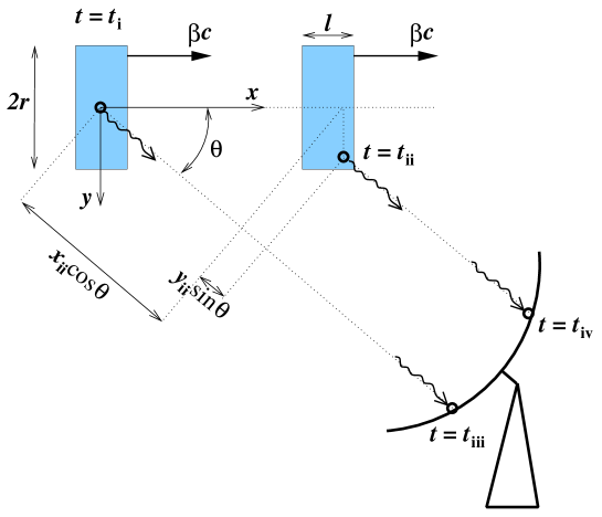
Figure 1: Cylindrical emission region geometry.

In this paper, I shall assume that the distance between the AGN and the observer is very much larger than the dimensions of the emission region ($R$ and $\ell$ in Fig. 1), and that we are not concerned with investigating variability on time scales very much shorter than $R/c$ or $\ell/c$. Under this assumption, the time interval between arrival of the two photons at the telescope is independent of distance to the AGN and is simply given by

$$t_{\rm obs}\equiv(t_{\rm iv}-t_{\rm iii})=\left(t_{\rm ii}-{x_{\rm ii}\over c}\cos\theta-{y_{\rm ii}\over c}\sin\theta\right).$$ (1)

The error made by using this approximation is $\sim(R/d_{L})(R/c)$ and is negligible compared with the variability time scale associated with the emission region geometry investigated in this paper which is $\sim(r/c)$.

Lorentz transformation to the observer frame, gives $t_{\rm ii}=\Gamma(t^{\prime}_{\rm ii}+\beta x^{\prime}_{\rm ii})$, $x_{\rm ii}=\Gamma(x^{\prime}_{\rm ii}+\beta t^{\prime}_{\rm ii})$ and $y_{\rm ii}=y^{\prime}_{\rm ii}$. Noting that the Doppler factor is $D=[\Gamma(1-\beta\cos\theta)]^{-1}=\Gamma(1+\beta\cos\theta^{\prime})$, and using the Aberration formulae,

$$\cos\theta = {\Gamma\over D}(\cos\theta^{\prime}+\beta),\;\;\;\sin\theta={1\over D}\sin\theta^{\prime}$$ (2)

$$\cos\theta^{\prime} = {\Gamma D}(\cos\theta-\beta),\;\;\;\sin\theta^{\prime}={D}\sin\theta,$$ (3)

Eq. 1 becomes

$$t_{\rm obs} = \Gamma(t^{\prime}_{\rm ii}+\beta x^{\prime}_{\rm ii})-\Gamma(x^{\prime}_{\rm ii}+\beta t^{\prime}_{\rm ii}){\Gamma\over Dc}(\cos\theta^{\prime}+\beta)-y^{\prime}_{\rm ii}{1\over Dc}\sin\theta^{\prime}$$ (4)

$$Dt_{\rm obs} = t^{\prime}_{\rm ii}-{x^{\prime}_{\rm ii}\over c}\cos\theta^{\prime}-{y^{\prime}_{\rm ii}\over c}\sin\theta^{\prime}.$$ (5)

Let us suppose that the cylindrical emission region emits radiation simultaneously and uniformly throughout its volume between times $t^{\prime}=-\Delta t^{\prime}$ and $t^{\prime}=\Delta t^{\prime}$, as measured in the jet frame. While a simultaneous burst violates causality, it is nevertheless a useful case to consider because it enables us to determine clearly the contribution of emission region geometry to the observed variability time. For $\theta^{\prime}\leq\pi/2$ the first photon to arrive would have been emitted at $(t^{\prime}=-\Delta t^{\prime},\,x^{\prime}=\ell^{\,\prime}/2,\,y^{\prime}=r,\,z^{\prime}=0)$ giving

$$t_{\rm obs}^{\rm first}=-\Delta t^{\prime}-(\ell^{\,\prime}/2c)\cos\theta^{\prime}-(r/c)\sin\theta^{\prime}.$$ (6)

Similarly, the last photon to arrive would have been emitted at $(t^{\prime}=\Delta t^{\prime},\,x^{\prime}=-\ell^{\,\prime}/2,\,y^{\prime}=-r,\,z^{\prime}=0)$ giving

$$t_{\rm obs}^{\rm last}=\Delta t^{\prime}+(\ell^{\,\prime}/2c)\cos\theta^{\prime}+(r/c)\sin\theta^{\prime}.$$ (7)

For $\theta^{\prime}>\pi/2$ the first photon to arrive would have been emitted at $(t^{\prime}=-\Delta t^{\prime},\,x^{\prime}=-\ell^{\,\prime}/2,\,y^{\prime}=r,\,z^{\prime}=0)$, and the last photon to arrive would have been emitted at $(t^{\prime}=\Delta t^{\prime},\,x^{\prime}=\ell^{\,\prime}/2,\,y^{\prime}=-r,\,z^{\prime}=0)$. Hence, if we define the observer frame duration of the burst as $2\Delta t_{\rm obs}$ then

$$D\Delta t_{\rm obs}=\Delta t^{\prime}+(\ell^{\,\prime}/2c)|\cos\theta^{\prime}|+(r/c)\sin\theta^{\prime}$$ (8)

and this is valid for all $\theta^{\prime}$. Note that Eq. 8 gives the usual formula, $\Delta t_{\rm obs}=\Delta t^{\prime}/D$, if the emission region is point-like (i.e. $\ell^{\,\prime}=r=0$). If one term in Eq. 8 dominates, $D\Delta t_{\rm obs}$ gives one of: $\Delta t^{\prime}$, $(\ell^{\,\prime}/2c)|\cos\theta^{\prime}|$, or $(r/c)\sin\theta^{\prime}$.

I shall next consider the case of a cylindrical emission region in the jet being rapidly energized by a plane shock with jet-frame speed $\beta^{\prime}_{\rm shock}c$ travelling along the jet, such that photons are emitted immediately after shock passage from a thin disk-like region immediately downstream of the shock. In this case, the location of the emitting disk is defined by $x^{\prime}=\beta^{\prime}_{\rm shock}ct^{\prime}$, and so the arrival times of photons at the telescope may be obtained from Eq. 5

$$cDt_{\rm obs} = x^{\prime}\left({1\over\beta^{\prime}_{\rm shock}}-\cos\theta^{\prime}\right)-y^{\prime}\sin\theta^{\prime}.$$ (9)

For $({1/\beta^{\prime}_{\rm shock}}-\cos\theta^{\prime})<1$ the first and last photons to be received would have been emitted at $(x^{\prime}=\ell^{\,\prime}/2,y^{\prime}=r,z^{\prime}=0)$ and $(x^{\prime}=-\ell^{\,\prime}/2,y^{\prime}=-r,z^{\prime}=0)$, respectively. However, for $({1/\beta^{\prime}_{\rm shock}}-\cos\theta^{\prime})>1$ the first and last photons to be received would have been emitted at $(x^{\prime}=-\ell^{\,\prime}/2,y^{\prime}=r,z^{\prime}=0)$ and $(x^{\prime}=\ell^{\,\prime}/2,y^{\prime}=-r,z^{\prime}=0)$, respectively. Hence, the observer frame duration of the burst is

$$D\Delta t_{\rm obs}=(\ell^{\,\prime}/2c)\left|{1\over\beta^{\prime}_{\rm shock}}-\cos\theta^{\prime}\right|+(r/c)\sin\theta^{\prime}.$$ (10)

If $\theta^{\prime}$ is small ($\theta$ is very small), one finds

$$\Delta t_{\rm obs} \approx {\ell^{\,\prime}\over 2Dc}\left|{1-\beta^{\prime}_{\rm shock}\over\beta^{\prime}_{\rm shock}}\right|+{r\theta^{\prime}\over Dc}$$ (11)

and for a reasonable shock speed, e.g. $\beta^{\prime}_{\rm shock}\sim\pm 0.5$,

$$\Delta t_{\rm obs} {\sim} (2\mp 1){\ell^{\,\prime}\over 2Dc}+{r\theta^{\prime}\over Dc}$$ (12)

where $\beta^{\prime}_{\rm shock}\sim-0.5$ corresponds to a reverse shock.

What we have learned from this discussion is that multiplying $c\Delta t_{\rm obs}$ by the Doppler factor might give the jet-frame intrinsic variability time or one of the dimensions of the emission region (possibly multiplied by some unknown factor). One is tempted to ask if ${R^{\prime}}\approx Dc\Delta t_{\rm obs}$ is the right dimension to put in $U^{\prime}_{\rm phot}=L^{\prime}/4\pi{R^{\prime}}^{2}c$ in order to estimate the jet-frame photon energy density. We shall discuss this point further in Section 4.

3 Monte Carlo investigation of $c\Delta t_{\rm obs}$, size, and $D$

The Monte Carlo method allows the accurate calculation of expected light curves for any emission region geometry and intrinsic source variability. The emission region is modeled in the jet frame, and is represented by $N$ “particles”, each of which emits precisely one “photon”. The number density of the particles models the geometry of the emission region, and each particle emits its photon at a time determined by the emission region geometry and variability model. The jet-frame 4-position of each photon emission event $(t^{\prime}_{i},x^{\prime}_{i},y^{\prime}_{i},z^{\prime}_{i})$, $i=1,2,\dots N$, is determined by model. The emission region moves in the $x$-direction with Lorentz factor $\Gamma$, and the observer-frame 4-position of each photon emission event $(t_{i},x_{i},y_{i},z_{i})$, $i=1,2,\dots N$, is obtained by Lorentz transformation. The arrival time of each photon is calculated for a given viewing angle $\theta$ using Eq. 1, and is binned to give the lightcurve.

Two emission region geometries are considered: a solid cylinder, and a spheroidal 3D gaussian. We also consider four intrinsic jet-frame time distributions: a simultaneous burst (violates causality), a simultaneous gaussian pulse (violates causality) and simultaneous emission at plane shock. I shall investigate effects of varying the Doppler factor $D$, viewing angle $\theta$, jet Lorentz factor $\Gamma$, and shock speed $\beta_{\rm shock}$. Finally, the effect of smoothing due to acceleration/radiation time delays is discussed.

3.1 Solid cylinder emission region geometry

If the emission region is “solid”, i.e. the emissivity is constant inside the emission region and zero outside, the lightcurve may be peaked and have finite duration to reflect the sharp edges of the emission region, and the shape of the lightcurve will change with with viewing angle. The Monte Carlo results for the cylinder, when plotted such that the time of observation is divided by the expected variability time $\Delta t_{\rm obs}$ given by Eqs. 8 and 10, is shown in Fig. 2(a) for a simultaneous burst ($\Delta t^{\prime}=0$) , and in Fig. 2(b) for shock excitation. As can be seen, Eqs. 8 and 10 are verified by the Monte Carlo results. In both cases the shape of the lightcurve depends strongly on the viewing angle.

Figure 2: Lightcurve from cylindrical emission region with $\ell/2r=0.1$ moving with Lorentz factor $\Gamma=10$ as observed at various viewing angles: (a) Simultaneous burst for $\theta^{\prime}=0^{\circ}$ (solid), $36^{\circ}$ (dotted), $72^{\circ}$ (short-dashed), $108^{\circ}$ (short-dashed, identical to $72^{\circ}$), $144^{\circ}$ (dotted, identical to $36^{\circ}$), $\theta^{\prime}=360^{\circ}$ (long-dash, identical to $0^{\circ}$); (b) Excitation by a plane shock moving at speed $\beta^{\prime}_{\rm shock}c=0.5c$ for $\theta^{\prime}=0^{\circ}$ (solid), $36^{\circ}$ (dotted), $72^{\circ}$ (short-dash), $108^{\circ}$ (dot-dash), $144^{\circ}$ (dot-dot-dot-dash), $\theta^{\prime}=360^{\circ}$ (long-dash, identical to $0^{\circ}$).

3.2 Gaussian emission region geometries

The density of “particles” representing the emission region is described by

$$\rho(x^{\prime},y^{\prime},z^{\prime})\propto\exp\left[-\;\left({{x^{\prime}}^{2}\over 2{\sigma_{x}}^{2}}+{{y^{\prime}}^{2}+{z^{\prime}}^{2}\over 2{\sigma_{r}}^{2}}\right)\right]$$ (13)

with $\sigma_{x}=\sigma_{r}$ corresponding to a spherical gaussian distribution, $\sigma_{x}<\sigma_{r}$ to an oblate spheroidal gaussian distribution, and $\sigma_{x}>\sigma_{r}$ to an prolate spheroidal gaussian distribution. For the case of a simultaneous gaussian pulse, the probability of emission at jet-frame time $t^{\prime}$ to $(t^{\prime}+dt^{\prime})$ is $p(t^{\prime})dt^{\prime}$, where $p(t^{\prime})=\exp(-{{t^{\prime}}^{2}/2{\sigma_{t}}^{2}})/\sqrt{2\pi}\sigma_{t}$ is independent of position.

If the emission region has a gaussian shape the lightcurve will be smooth, and in many cases will also have a gaussian shape. This is true, for example, for the cases of a simultaneous gaussian pulse and excitation by a plane shock. The width of the lightcurve will depend on viewing angle in approximately the same way as for equivalent cylindrical emission volume. For example, $r$ and $\ell^{\prime}/2$ of the solid cylinder should be related to $\sigma_{r}$ and $\sigma_{x}$, respectively, for the case of the spheroidal gaussian density. For the case of a simultaneous gaussian burst I find the standard deviation to be given by

$$\sigma=[(\sigma_{r}\sin\theta^{\prime}/c)^{2}+(\sigma_{x}\cos\theta^{\prime}/c)^{2}+\sigma_{t}^{2}]^{1/2}/D.$$ (14)

Note the similarity to Eq. 8 except that the terms are added in quadrature as the standard deviation is required instead of the maximum duration of the pulse which is, theoretically, infinite.

In the case of excitation by a plane shock wave with speed $\beta_{\rm shock}c$, the emission is from the plane where the shock cuts the spherical gaussian density. The emission region then has a surface density of emitting particles which is a two-dimensional gaussian, and the lightcurve reflects this distribution, and so is also gaussian. The standard deviation of the gaussian lightcurve depends on the viewing angle as a result of projection effects, and I find the standard deviation to be

$$\sigma={1\over cD}\left[(\sigma_{r}\sin\theta^{\prime})^{2}+(\sigma_{x})^{2}\left({1\over\beta^{\prime}_{\rm shock}}-\cos\theta^{\prime}\right)^{2}\right]^{1/2}$$ (15)

Lightcurves for $\Gamma=10$, $\beta^{\prime}_{\rm shock}=0.5$ and various viewing angles are plotted in Fig. 3 and seen to lie on top of each other when plotted in units of $\sigma$, and to be a normal distribution. Equation 15 is valid for both forward and reverse shocks. For reverse shocks, $\beta^{\prime}_{\rm shock}$ would be negative and give rise to a broader lightcurves (larger $\sigma$).

Figure 3: Lightcurve due to excitation by a plane shock of a spherical density moving with Lorentz factor $\Gamma=10$ for $\beta^{\prime}_{\rm shock}=0.5$ and various viewing angles shown is seen to be a normal distribution.

3.3 Acceleration/radiation delays

Instantaneous excitation by a shock wave is not a realistic approximation unless the time-scales for particle acceleration and radiation (cooling) are very short compared to the transit time of the shock through the emission region. If this is not the case, the lightcurve would be broadened and smoothed to reflect the time delays associated with particle acceleration and radiation. An equation of the form $dN^{\prime}/dt^{\prime}=Q^{\prime}(t^{\prime})-N^{\prime}/t^{\prime}_{\rm loss}$ might describe the time-evolution of the number of particles, $N^{\prime}$, radiating photons at the frequency corresponding to that observed, with $Q^{\prime}(t^{\prime})$ being the source term, and $t^{\prime}_{\rm loss}$ representing the time-scale for particle losses (or time-scale over which the radiation is emitted). Then a simple smoothing function of the form

$$\phi_{\rm del}(t^{\prime}_{\rm del})=\left\{\begin{array}[]{ll}0&(t^{\prime}_{\rm del}<0)\\ {1\over\Delta t^{\prime}_{\rm gain}}\left[1-\exp\left({-t^{\prime}_{\rm del}\over t^{\prime}_{\rm loss}}\right)\right]&(0\leq t^{\prime}_{\rm del}<\Delta t^{\prime}_{\rm gain})\\ {1\over\Delta t^{\prime}_{\rm gain}}\left[1-\exp\left({-\Delta t^{\prime}_{\rm gain}\over t^{\prime}_{\rm loss}}\right)\right]\exp\left[{-(t^{\prime}_{\rm del}-\Delta t^{\prime}_{\rm gain})\over t^{\prime}_{\rm loss}}\right]&(\Delta t^{\prime}_{\rm gain}\leq t^{\prime}_{\rm del})\end{array}\right.$$ (16)

can be used for this purpose, where $t^{\prime}_{\rm del}$ represents the delay between shock passage and emission by the radiating particles, $\Delta t^{\prime}_{\rm gain}$ represents the the duration of the acceleration following shock passage. In the case of a pre-existing population of thermal electrons shock heating is essentially instantaneous ($\Delta t^{\prime}_{\rm gain}=0$), and $t^{\prime}_{\rm loss}$ represents the time-scale for cooling by thermal bremsstrahlung radiation. Similarly, for a pre-existing population of relativistic electrons, the passage of the shock will essentially instantly increase the magnetic field ($\Delta t^{\prime}_{\rm gain}=0$) and $t^{\prime}_{\rm loss}$ would represent the time-scale for energy losses by synchrotron emission. If particle acceleration is required then $\Delta t^{\prime}_{\rm gain}>0$.

Figure 4: Excitation of an oblate spheroidal gaussian density ($\sigma_{x}/\sigma_{r}=0.2$) moving with Lorentz factor $\Gamma=10$ by a plane shock with jet-frame speed $\beta^{\prime}_{\rm shock}c=0.3c$, followed by particle acceleration and radiation represented by Eq. 16 with $\Delta t^{\prime}_{\rm gain}=t^{\prime}_{\rm loss}$ for $t^{\prime}_{\rm loss}=0.1\sigma_{r}/c$, $\sigma_{r}/c$ and $10\sigma_{r}/c$ (as indicated) for viewing angle $\theta=5^{\circ}$. Solid curves give the result of convolution (Eqn. 18).

Fig. 4 shows the effect of acceleration/radiation delays on the lightcurve due to a plane shock ($\beta^{\prime}_{\rm shock}=0.3$) exciting an oblate gaussian spheroidal emission region ($\sigma_{x}/\sigma_{r}=0.2$) with acceleration/radiation delays described by $\Delta t^{\prime}_{\rm gain}=t^{\prime}_{\rm loss}$ for $t^{\prime}_{\rm loss}=0.1\sigma_{r}/c$, $\sigma_{r}/c$ and $10\sigma_{r}/c$, and viewed at angle $\theta^{\prime}=5^{\circ}$. In the case of no acceleration/radiation delays, the lightcurves would simply be normal distributions centred on $t_{\rm obs}=0$. Results are shown for the three $t^{\prime}_{\rm loss}$-values, and $t_{\rm obs}$ is plotted in terms of $\sigma_{\rm tot}$ defined by

$$\sigma_{\rm tot}^{2}=\sigma^{2}+{{t^{\prime}_{\rm loss}}^{2}+{\Delta t^{\prime}_{\rm gain}}^{2}\over 4cD},$$ (17)

where $\sigma$ is given by Eqn. 15, such that $\sigma_{\rm tot}$ gives a crude measure of the expected duration of the lightcurve. These distributions can be obtained simply by convolution of a normal distribution with $\phi_{\rm del}$ (Eq. 16), taking account of the fact that jet-frame times enter in Eq. 16, that for any point co-moving with the jet $\Delta t_{\rm obs}=\Delta t^{\prime}/D$, and that $t_{\rm obs}$ is plotted in units of $\sigma_{\rm tot}$,

$$p\left({t_{\rm obs}\over\sigma_{\rm tot}}\right)={\sigma D\over\sqrt{2\pi}}\int_{-\infty}^{\infty}\phi_{\rm del}(t_{\rm obs}D-t)\exp\left({-t^{2}\sigma_{\rm tot}^{2}\over 2\sigma^{2}}\right)dt.$$ (18)

The solid curves, which agree with the Monte Carlo results (histograms), are obtained from Eqn. 18. As we see, if the time-scales for the acceleration/radiation process ($\Delta t^{\prime}_{\rm gain}$ and $t^{\prime}_{\rm loss}$) are much less than the time-scale $\sigma^{\prime}$ associated with the shock passage and dimensions of the emission region then the light-curve will be symmetrical, and in the case of a gausian spheroidal emission region will be a gaussian distribution with standard deviation $\sigma$ (leftmost histogram). If the time-scales for the acceleration/radiation process are much larger than $\sigma^{\prime}$, then the light-curve will reflect that of the acceleration/radiation process, i.e. Eqn. 16 (rightmost histogram). The middle histogram shows an intermediate case.

Lightcurves of AGN show many different features and forms of variability. One example which appears to show variations reflecting the acceleration/radiation process is 3C 454.3. In Fig. 5, I show the lightcurve of 3C 454.3 at 37 GHz obtained with the Metsahovi and Crimea telescopes over ten years (Salonen et al. 1987, Terasranta et al. 1992). The flares appear non-symmetrical and have a shape similar to the rightmost histogram in Fig. 4 ($\Delta t^{\prime}_{\rm gain}=t^{\prime}_{\rm loss}\gg\sigma$). As an example, I have constructed a reasonably well-fitting lightcurve (solid curve) from a number of flares of the form given by Eqn. 16 with $\Delta t_{\rm gain}=t_{\rm loss}=0.75$ yr (dotted curves) plus a background flux density of 3 Jy. One interpretation of these data would then be that the radio emission region in 3C 454.3, being modelled by the solid curve, has dimensions much less than $c$(0.75 yr)$D=0.16D$ pc, and that the energy-loss time-scale of the radiating electrons is $\sim$(0.75 yr)$D$.

Figure 5: Lightcurve of 3C 454.3 at 37 GHz (Salonen et al. 1987, Terasranta et al. 1992). The fit (solid curve) comprises a background level (horizontal dotted line) and several flare components (dotted curves) with individual flare lightcurves given by Eq. 16 with $\Delta t_{\rm gain}=t_{\rm loss}=0.75$ yr.

Another example is the X-ray lightcurve of 1ES1959+65 from ARGOS/USA and RXTE/ASM (Giebels et al. 2002) shown in Fig. 6. In this case, the individual flares appear to be symmetrical in time, and have a roughly gaussian shape. I have constructed a reasonably well-fitting lightcurve (solid curve) from a number of flares of gaussian form with standard deviations $\sigma=2.5$ d (dotted curves) plus a background flux density of 2 mCrab. One could interpret this as indicating that the energy-loss time-scale of the radiating electrons is much less than $2.5D$ d, and that the emission region dimensions are $\sim c2.5D$ d$=2\times 10^{-3}D$ pc.

Figure 6: X-ray lightcurve of 1ES1959+65 (Giebels et al. 2002). The fit (solid curve) comprises a background level (horizontal dotted line) and several flare components (dotted curves) with individual gaussian lightcurves with standard deviations $\sigma=2.5$ d.

4 Dependence of energy density on dimensions of the blob

It is important to know the dimensions of the emission region for several reasons: (i) in some hadronic models the synchrotron photons are targets for photoproduction, (ii) in all models the synchrotron photons are targets for photon-photon pair production by $\gamma$-rays, (iii) in SSC models the synchrotron photon energy density determines Compton scattering, and (iv) knowing the systematic errors on photon energy density may help understand the so-called “Compton catastrophe” in IDV sources which have apparent brightness temperatures well in excess of the limit $T_{B}<10^{12}$ K imposed by Compton scattering (Kellermann and Pauliny-Toth 1969, Kardashev 2000) when the photon energy density in the emission region reaches the energy density in the magnetic field. One extreme example is PKS 0405-385 (Kedziora-Chudczer et al. 1997) which has $T_{B}>5\times 10^{14}$ K after correcting for interstellar scintillation (see also Walker 1998) requiring a Doppler factor of $D=10^{3}$ to satisfy the brightness temperature limit.

To illustrate how critically the energy density depends on the geometry, I shall consider the case of the jet-frame emissivity following a spheroidal gaussian density. Provided the emission is optically thin, as is almost certainly true for the optical–X-ray synchrotron hump in the SED of blazars, then it is straightforward to calculate the average energy density from the emission region geometry and the luminosity.

Assuming that the jet-frame luminosity, $L^{\prime}$, is constant, we can estimate the average jet-frame photon energy density given the Doppler factor and emission region geometry. The simplest way of doing this, for any emission region geometry, is to use the Monte Carlo method to place $N$ points at positions $\vec{r}_{i},\;i=1,\dots N$, distributed according to the emission region geometry, and to give each point a luminosity $L^{\prime}/N$. Then at point $\vec{r}_{i}$ the energy density is

$$U^{\prime}_{\rm phot}(\vec{r}_{i})\approx{L^{\prime}\over 4\pi cN}\sum_{j\neq i}r_{ij}^{-2}$$ (19)

where $r_{ij}=|\vec{r}_{i}-\vec{r}_{j}|$. Averaging over the emission region distribution we obtain

$$\langle U^{\prime}_{\rm phot}\rangle\approx{L^{\prime}\over 4\pi cN^{2}}\sum_{i=1}^{N}\sum_{j\neq i}r_{ij}^{-2}.$$ (20)

The result giving the jet-frame average photon energy density versus $\sigma_{x}$ is shown as the thick solid curve in Fig. 7 for the case of a gaussian spheroidal density.

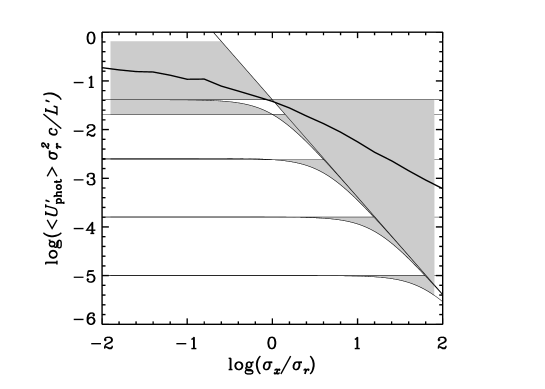
Figure 7: Jet-frame average photon energy density versus $\sigma_{x}$. Thick solid curve shows actual density calculated using the Monte Carlo method. “Observed” density is shown by the shaded areas for $\sigma_{t}=0$ (top shaded area), $\sigma_{r}$, 4$\sigma_{r}$, 8$\sigma_{r}$, and $16\sigma_{r}$ (bottom shaded area). See text for further details.

In Fig. 7 we also plot the jet-frame average photon energy density that would be inferred if we assumed that the observed variability time scale $\sigma$ and an assumed or estimated Doppler factor $D$ gave the jet-frame radius of a spherical emission region, i.e. $R^{\prime}=\sigma Dc$. This “observed” jet-frame average photon energy density is simply given by

$$\langle U^{\prime}_{\rm phot,\,obs}\rangle\equiv{L^{\prime}\over 4\pi(\sigma Dc)^{2}c}.$$ (21)

Note that $\sigma$ (given by Eq. 14) depends on $\theta^{\prime}$, $\sigma_{t}$ and $\sigma_{x}$ so that the “observed” jet-frame average photon energy density depends also on $\theta^{\prime}$, $\sigma_{t}$ and $\sigma_{x}$ as well as $D$. The figure shows $\langle U^{\prime}_{\rm phot,\,obs}\rangle$ plotted against $\sigma_{x}$ and gives the range due to variation in $\theta^{\prime}$ (shaded) for various $\sigma_{t}$. The upper bound in each case gives the result for $\theta^{\prime}=0$ or $\pi$ and the lower bound is for $\theta^{\prime}=\pi/2$. We see that the “observed” value, $\langle U^{\prime}_{\rm phot,\,obs}\rangle$ can be several orders of magnitude higher or lower than $\langle U^{\prime}_{\rm phot}\rangle$ if the emission region is different from a sphere, or if the intrinsic variability time $\sigma_{t}$ is not small. For example, take the case of $\sigma_{t}\ll\sigma_{r}/c$, if $\sigma_{x}=10^{-2}\sigma_{r}$ and $\theta^{\prime}=0$ ($\theta=0$) then $\langle U^{\prime}_{\rm phot,\,obs}\rangle\approx 10^{3}\langle U^{\prime}_{\rm phot}\rangle$, whereas if $\sigma_{x}=10^{2}\sigma_{r}$ and $\theta^{\prime}=90^{\circ}$ ($\theta=5.74^{\circ}$ for $\Gamma=10$) then $\langle U^{\prime}_{\rm phot,\,obs}\rangle\approx 10^{2}\langle U^{\prime}_{\rm phot}\rangle$. The above result has clear implications for both leptonic and hadronic models of AGN in which photons of the low-energy peak of the SED provide target photons for inverse-Compton scattering by electrons (leptonic models) or pion photoproduction by protons (hadronic models). Using the observed variability time together with assumed or estimated Doppler factor to estimate the emission region radius $R^{\prime}$ can clearly lead to large errors in $\langle U^{\prime}_{\rm phot}\rangle$.

Although the radio emission in IDV sources is usually assumed to be optically thick, if this is not the case then the above result may also have implications for IDV sources as the photon energy density responsible for causing the brightness temperature limit may actually be a few orders of magnitude lower than estimated on the basis of time-variability, and in that case much lower Doppler factors would be required to avoid the Compton catastrophe. I explore this further in a separate paper (Protheroe 2002).

5 Variability due to photon pile-up in observation time

The simplest example of photon pile-up in observation time is a bent jet. Jets may bend if they pass through a stratified cold and high density region (Mendoza and Longair 2001). We approximate the trajectory of an emission region moving with speed $\beta c=(1-1/\Gamma^{2})^{-1/2}$ along a bent section of jet by motion around a section of a circle of radius $r$ in the $x$–$y$ plane: $(t,\,x=r\cos(\omega t),\,y=r\sin(\omega t),\,z=0)$, where $\omega=\beta c/r$. For an observer in the $x$–$z$ plane at angle $\eta$ to the $x$-axis, the observation time is then given by

$$t_{\rm obs}=t-(r/c)\cos(\omega t)\cos\eta$$ (22)

and the Doppler factor is

$$D=\{\Gamma[1+\beta\cos\eta\sin(\omega t)]\}^{-1}.$$ (23)

The Doppler factor raised to the 4th power is plotted against observation time for $\Gamma=10$ and various observation angles in Fig. 8. I have plotted $D^{4}$ as it is appropriate for bolometric flux from a moving isotropic source; it also applies to the specific flux $F_{\nu}$ for $F_{\nu}\propto\nu^{-1}$. We see that even for modest observation angles the lightcurve is strongly peaked, essentially a delta function when the emission region direction is closest to the line of sight. Of course the finite size of any emission region will broaden the distribution. For example, for a lab-frame emission region length along the jet $\ell$, the burst would have duration $\Delta t_{\rm obs}\sim\ell/c$.

Figure 8: Doppler factor raised to 4th power representing bolometric lightcurve due to emission region moving along a bent jet. The jet Lorentz factor is $\Gamma=10$, the bent jet is approximated by part of a circle around which jet plasma moves with angular velocity $\omega$, and the emission region is observed at angle $\eta\leq 0.3^{\circ}$ (solid curve), $\eta=27^{\circ}$ (chain curve), $\eta=81^{\circ}$ (dashed curve).

5.1 Helical jet structures

Figure 9: Shock excited helical jet structure for $\Gamma=10$, $\beta^{\prime}_{\rm shock}=0.5$, $\lambda=r$. (a) $t^{\prime}$ vs. $t_{\rm obs}$ for $\theta=0.3^{\circ}$ (solid curve), $1^{\circ}$ (dotted curve), $3^{\circ}$ (short dashed curve), $9^{\circ}$ (dot-dash curve), and $27^{\circ}$ (dot-dot-dot-dash curve). Resulting lightcurves for (b) $\theta=0.3^{\circ}$, (c) $1^{\circ}$, (d) $3^{\circ}$, (e) $9^{\circ}$, and (f) $27^{\circ}$.

VLBI observations show that helical jets or helical structures in jets may be fairly common in AGN (Rantakyro et al. 1998), and theoretical studies have shown that wave-like helical structures can occur as a result of jet precession (Hardee 2000). Several papers discuss helical jet models or the application of helical models to specific sources (Camenzind 1986, Rosen 1990, Tateyama et al. 1998, Qian et al. 1992, Schramm et al. 1993, Steffen et al. 1995, Villata and Raiteri 1999). Certainly helical jets or structures would be important in determining the lightcurve of $\gamma$-ray and neutrino emission from blazars, and various suggestions have been made about the mechanisms involved (Despringre and Fraix-Burnet 1997, Marcowith et al. 1995).

I consider a filamentary helical structure embedded in the jet with Lorentz factor $\Gamma$ whose axis coincides with the jet axis and is excited by a plane shock travelling along the jet with jet-frame speed $\beta^{\prime}_{\rm shock}c$. The helical structure could be, for example, a flux tube containing a relatively high magnetic field, or a tube of high plasma density arising from a density perturbation in the plasma entering the jet. Helical magnetic fields with an Archemedian spiral topology similar to the “Parker spiral” field of the heliosphere may well be expected in AGN jets.

The excitation of a filamentary helical structure is described by the jet-frame 4-vector $(t^{\prime},x^{\prime},y^{\prime},z^{\prime})=(\lambda\!\!\!^{-}\phi/\beta^{\prime}_{\rm shock}c,\,\lambda\!\!\!^{-}\phi,\,r\cos\phi,\,r\sin\phi)$, where $r$ is the radius of the cylinder containing the helix, $\lambda$ is the helix wavelength, $\lambda\!\!\!^{-}=\lambda/2\pi$, $\phi=\beta^{\prime}_{\rm shock}ct^{\prime}/\lambda\!\!\!^{-}$, and the jet is pointing in the $x$-direction. Lorentz transformation to the galaxy-frame gives $(t,x,y,z)=[\Gamma t^{\prime}(1+\beta\beta^{\prime}_{\rm shock}),\,\Gamma ct^{\prime}(\beta+\beta^{\prime}_{\rm shock}),\,r\cos(\beta^{\prime}_{\rm shock}ct^{\prime}/\lambda\!\!\!^{-}),\,r\sin(\beta^{\prime}_{\rm shock}ct^{\prime}/\lambda\!\!\!^{-})]$. The galaxy-frame speed of the location of the excited part of the helix can exceed $c$, but this does not violate causality as no particles or information propagates at this pattern speed which is

$$v_{\rm pattern}={\beta^{\prime}_{\rm shock}+\beta\over 1+\beta^{\prime}_{\rm shock}\beta}\left[1+\left({r\beta^{\prime}_{\rm shock}\over\lambda\!\!\!^{-}\Gamma(\beta^{\prime}_{\rm shock}+\beta)}\right)\right]c.$$ (24)

Observation in the $x$-$z$ plane at angle $\theta$ to the jet axis ($x$-axis) gives

$$t_{\rm obs} = \Gamma t^{\prime}[1+\beta\beta^{\prime}_{\rm shock}-(\beta^{\prime}_{\rm shock}+\beta)\cos\theta]+r\sin\theta\sin(\beta^{\prime}_{\rm shock}ct^{\prime}/\lambda\!\!\!^{-})/c$$ (25)

$${dt_{\rm obs}\over dt^{\prime}} = \Gamma[1+\beta\beta^{\prime}_{\rm shock}-\cos\theta(\beta^{\prime}_{\rm shock}+\beta)]+r\sin\theta\,(\beta^{\prime}_{\rm shock}/\lambda\!\!\!^{-})\cos(\beta^{\prime}_{\rm shock}ct^{\prime}/\lambda\!\!\!^{-}).$$ (26)

Whenever $dt_{\rm obs}/dt^{\prime}=0$ the lightcurve will have a cusp. If cusps are possible, they will occur at times corresponding to

$$\cos\phi = {-\Gamma[1+\beta\beta^{\prime}_{\rm shock}-\cos\theta(\beta^{\prime}_{\rm shock}+\beta)]\over r\sin\theta\,(\beta^{\prime}_{\rm shock}/\lambda\!\!\!^{-})}$$ (27)

provided the model parameters give $\cos\phi$ in the range $-1\leq\cos\phi\leq 1$ ($\cos\phi$ depends on the helix geometry, shock speed, jet Lorentz factor and viewing angle). If $\cos\phi=\pm 1$ one cusp per helix wavelength will occur, and if $-1<\cos\phi<1$ multiple cusps occur, otherwise no cusps are present in the light curve. However, if $\cos\phi$ is close to $\pm 1$ the lightcurve will be peaked. This is illustrated in Fig. 9 for $\Gamma=10$, $\beta^{\prime}_{\rm shock}=0.5$, and $\lambda=r$. Fig. 9(a) shows $t^{\prime}$ plotted against $t_{\rm obs}$ for five viewing angles, and Fig. 9(b)–(f) shows the resulting lightcurve for each of the five viewing angles (the corresponding Doppler factors are also given).

Apart from the periodicity, the lightcurves shown in Fig. 9 are reminiscent of those of blazars. All of these lightcurves correspond to instantaneous emission from the point on the helical filament at the time of excitation. The cusps and peaks would in reality be smoothed to some extent by the finite width of any helical structure as well as by any delays associated with acceleration and radiation time scales. Furthermore, as the shock weakens while propagating down the jet the successive peaks/cusps in the lightcurve would decrease in height. One possible scenario could be that there is a succession of shocks at random intervals propagate down the jet, and because individual shocks weaken as they propagate, each shock would cause only one or two peaks (due to only one or two cycles of the helix). In this case, it may not be possible to distinguish between a simple bent structure in the jet and a helical structure – if appropriately aligned, a simple bent structure would cause a cusp in the lightcurve in exactly the same way as a helical structure. An alternative to a helical filamentary structure within the jet is a helical jet which would produce a qualitatively-similar lightcurve, but would have the Doppler factor varying with position along the jet as the viewing angle relative to the local jet direction changes.

5.2 Conical shocks

Lind and Bladford (1985) have considered the possibility that hotspots seen in VLBI images of radio jets may actually be relativistically moving conical shocks. They applied the relativistic shock jump conditions to a plane parallel flow entering a forward conical shock with cone angle $\eta$ to find the angle $\zeta<\eta$ with at which the flow initially diverges with respect to the jet axis. Defining the downstream region between the cones with angles $\zeta$ and $\eta$ to be the emission region, and taking account of Doppler boosting, they model the brightness distribution to simulate VLBI images.

The generation of conical shock structures is often seen to occur in simulations of relativistic jets after the introduction of a fast perturbation (Bowman 1994, Gomez et al. 1997). These structures, which are typically an alternating sequence of forward and reverse conical shocks, are stationary or slowly-moving in the galaxy frame, and have cone angles $\eta\sim 1/\Gamma$. Salvati et al. (1998) discuss emission by a conical shock. They consider the case of a density perturbation, confined to thin flat disk, travelling relativistically along the jet causing particle acceleration and emission where the disk cuts a stationary forward conical shock such as that illustrated in Fig. 10.

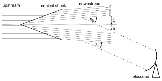
Figure 10: Side view of the jet showing the location of a stationary forward conical shock, and showing the downstream flow diverging from the jet axis at angle $\zeta$ (not to scale). For a viewing angle $\theta$ with respect to the jet axis, the angle between the downstream flow direction and the line of sight varies between $\theta_{a}$ and $\theta_{b}$.

Salvati et al. (1998) assume that the time-scales for acceleration and emission are negligible. They show that their model can lead to highly peaked light curves whose shape depends on the viewing angle, and used these light curves to fit Markarian 421 TeV flare data. For the same input, and assuming there is no Doppler boosting of the emitted radiation, I am able to reproduce exactly their figure 2 which shows the observed flux for various viewing angles. However, bearing in mind that the shock is stationary and that the pile-up in observing time is already included, the bolometric flux emitted by part of the downstream flow will be Doppler boosted by $D_{\rm local}^{3}$ where $D_{\rm local}=[\Gamma_{d}(1-\beta_{d}\cos\theta_{\rm local})]^{-1}$ where $\Gamma_{d}$ is the Lorentz factor of the downstream flow, and $\theta_{\rm local}$ is the viewing angle with respect to the line of sight and the local downstream flow direction which varies around the shock as indicated in Fig. 10 ($\theta_{\rm local}$ ranges between $\theta_{a}$ and $\theta_{b}$). To obtain the Lorentz factor of the downstream flow, it is easiest to Lorentz transform in a direction parallel to the shock plane to a frame in which the flow is normal to the shock. For the case of cone angle $\eta=\sin^{-1}(1/\Gamma)$ assumed by Salvati et al. (1998), i.e. an oblique shock at angle $\eta$ to the upstream flow, and using the relativistic equation of state, I find that for $\Gamma=10$, $\eta\approx 7.25^{\circ}$ and $\zeta\approx 1.89^{\circ}$ and that the Lorentz factor of the downstream flow is related to that of the upstream flow by $\Gamma_{d}\approx 0.801784\Gamma_{u}$. My result for the observed flux for the same input as Salvati et al., but including the Doppler boosting taking into account the local downstream flow directions, is given in Fig. 11(a) and shows that the inclusion of Doppler boosting causes the peak at $\theta=0$ to be higher than that at $\theta=0.9\eta$, the opposite to that found by Salvati et al. However, since Salvati et al. (1998) used one viewing angle in their fits to Markarian 421 TeV flare data (their figure 3), and because the divergence of the downstream flow is rather small, their fits are still valid and their model remains an interesting mechanism for flare production. The same authors (Spada et al. 1999) have applied their model to IDV sources and are able to explain brightness temperatures up to $3\times 10^{17}$ K.

Figure 11: Lightcurve of (a) a stationary forward conical shock and (b) a stationary reverse conical shock locally excited by a thin density perturbation travelling along the jet with Lorentz factor $\Gamma=10$ as viewed at angle $\theta$ with respect to the jet axis. The cone angle is $\eta=\sin^{-1}(1/\Gamma)$ and results are given for $\theta/\eta=0.001$ (long dashed curves), 0.1 (dot-dot-dot-dash curves), 0.3 (dot-dash curves), 0.5 (short dashed curves), 0.7 (dotted curves), 0.9 (solid curves). The Doppler factor is calculated using the local downstream flow velocity.

I wish to extend the work of Salvati et al. (1998) by including the reverse shocks, and ultimately a sequence of stationary reverse and forward shocks. In Fig. 11(b) I show the lightcurve for a reverse conical shock having identical parameters as the forward shock already discussed. Because the divergence of the downstream flow is rather small, the lightcurve of the reverse shock is approximately just the lightcurve of the forward shock reflected about $t_{\rm obs}=0$.

I shall consider next the case of a sequence of stationary reverse and forward conical shocks. Although in real AGN jets it may be possible that the downstream flow is re-accelerated to near the original value (depending on conditions external to the jet, and the jet production mechanism), I shall assume that each successive conical shock causes a reduction in the jet Lorentz factor by $\Gamma_{d}/\Gamma_{u}=0.801784$. I shall make an additional approximation that the divergence/convergence of the flow caused by the conical shocks can be neglected, and that the jet flow is always parallel to the jet axis. The lightcurve due to a thin, initially flat, disk travelling relativistically along the jet is then calculated by the Monte Carlo method, in which “particles” are placed over the surfaces of all of the cones. Each cone has the same number of particles, and they would appear uniformly distributed across the cross section of the jet when viewed along the jet axis. A side view showing the location of these particles is given in Fig. 12. An initially flat thin disk is launched along the jet with initial Lorentz factor $\Gamma=10$, and each time a part of the disk crosses one of the shocks the Lorentz factor of that part of the disk drops appropriately, distorting the disk. The time at which each “particle” emits its photon is determined by the time at which the (distorted) disk reaches the “particle”. The resulting lightcurve for various viewing angles is shown in Fig. 13(a) where the emission is boosted using the Doppler factor corresponding to the Lorentz factor of the flow immediately downstream of each shock. If the Lorentz factor of the jet decreases at each shock crossing as assumed here then, because the Doppler factor is also reduced at each shock crossing, only the first few conical shocks would be prominent in the lightcurve resulting from a single jet perturbation. This is shown in Fig 13(b) which gives the lightcurve from Fig 13(a) for $\theta=9^{\circ}$ on a linear scale.

Figure 12: Side view of the jet showing the location of “particles” used in the Monte Carlo Method. The location of the conical shocks is clearly evident.

Figure 13: Lightcurve due to excitation of the sequence of stationary conical conical shocks discussed in the text for an initial jet Lorentz factor $\Gamma=10$ (a) as seen at viewing angles $\theta=0^{\circ}$ (solid curve), $3^{\circ}$ (dotted curve), $6^{\circ}$ (short dashes), $9^{\circ}$ (dot-dash) and $12^{\circ}$ (dot-dot-dot-dash) with respect to the jet axis, and (b) as seen at viewing angles $\theta=9^{\circ}$ and plotted on a linear scale.

As can be seen, the lightcurve is quasi-periodic. It would be strictly periodic if the downstream flow velocity were identical to the upstream flow velocity. This might be the case if the re-collimmation of the diverging flow from the conical shocks results in restoration of the flow Lorentz factor to near the upstream value, and in this case the flux from successive cycles would be at about the same level, as observed in Markarian 501 flares. The two flow velocities would also be roughly the same if the initial jet Lorentz factor were much higher than $\Gamma=10$ used in Fig. 13(a) such that the intervals between flares due to a pair of conical shocks was roughly the same. However, in this case the flux of successive flares would diminish as the Doppler factor decreases. Turning this argument around, we may have a method of determining the minimum jet Lorentz factor from observational data, e.g. the $\sim 23$ day periodicity in the 1997 Markarian 501 data (Protheroe et al. 1998, Hayashida et al. 1998) may be used to put a lower limit on $\Gamma$.

Fig. 14 shows an example lightcurve due to multiple jet perturbations. In this case, I have used an exponential distribution of times between the injection into the jet of a density perturbation with a mean interval of $r/c$. I have also used an exponential distribution for the strength of each perturbation. The resulting lightcurve looks, at least qualitatively, as good as any model for the variability of fluxes from blazars. Note that even though there is no strict periodicity resulting from the excitation of a sequence of shocks in this case, each flare episode has two strong peaks due to (for this viewing angle) the apex of the first reverse shock cone and the apex of the first forward shock cone, and in each flare the separation between these two peaks is identical. Fourier analysis would therefore show a strong peak at the frequency corresponding to the time interval between these two peaks in a single flare.

Figure 14: Lightcurve due to repeated excitation of the sequence of stationary conical conical shocks discussed in the text for an initial jet Lorentz factor $\Gamma=10$ as seen at viewing angles $\theta=9^{\circ}$. The time interval between perturbations entering the jet is sampled from an exponential distribution with mean $r/c$, and the strength of the perturbation is also sampled from an exponential distribution.

6 Conclusion

Many factors can influence observed variability time. The connection between $\Delta t_{\rm obs}$, Doppler factor and emission region geometry is non-trivial, and so measuring $\Delta t_{\rm obs}$ may give, at best, one of the dimensions of the emission region. Using $R^{\prime}=c\Delta t_{\rm obs}D$ and $U^{\prime}_{\rm phot}=L^{\prime}/4\pi{R^{\prime}}^{2}c$ may then lead to over-estimation or under-estimtion of the jet-frame photon energy density by orders of magnitude. This is clearly of importance in any AGN model in which the low energy photons produced in the jet are targets for interaction of high energy particles or radiation, such as in SSC models and hadronic blazar models. Although not discussed in detail in the present paper, the escape of $\gamma$-rays from the emission region depends on the optical depth to photon-photon pair production interactions. This optical depth can be uncertain by orders of magnitude in the same way as the photon energy density, and will also depend on viewing angle. One must therefore be careful when using the observation of apparently unattenuated gamma-rays, and an observed variability time, to place limits on the Doppler factor.

The uncertainty in the jet-frame photon energy density discussed in this paper may also have implications for the high brightness temperature/Compton catastrophe problem of IDV sources. In this case, it is the energy density of target photons which limits the brightness temperature through the competition of inverse-Compton scattering with synchrotron radiation, and the target photon energy density may actually be lower than estimated if the emission region is non-spherical.

If the jet is bent or helical, or has some other favoured geometry (e.g. conical shocks) cusps in $t^{\prime}$ vs. $t_{\rm obs}$, and/or a varying Doppler factor may cause narrow peaks in the observed lightcurve irrespective of other factors. Distinguishing between these cases from the observed lightcurve alone is likely to be difficult. One way of distinguishing whether a flare is due to (i) an emission region moving around a bent or helical path, or (ii) a shock is exciting a curved, conical or helical structure within a jet, is that the in the first case the flare is caused by a change in viewing angle with respect to the motion of the emission region leading to a change in Doppler factor, whereas in the second case the flare is due to a pile-up in observation times with no change in Doppler factor. Hence, in case (i) not only will the observed flux increase during a flare, but the photon energies also increase – increase in $(\nu F_{\nu})_{\rm peak}$ by factor $x^{4}$ accompanied by shift in $\nu_{\rm peak}$ by factor $x$ ($x$ is ratio of final to initial Doppler factor). In case (ii), however, since there is no change in Doppler factor there should be no shift in $\nu_{\rm peak}$ accompanying an increase in $(\nu F_{\nu})_{\rm peak}$.

Distinguishing between the excitation of a conical and a helical structure by a plane shock would be almost impossible – note the qualitative similarities between lightcurves depicted in Figs. 9(d) and 13(b). Relativistic jet simulations (Bowman 1994, Gomez et al. 1997) do show the presence of conical shocks, and these shocks appear after a large perturbation (e.g. from 4 to 10 in the simulations of Gomez et al. 1997) in Lorentz factor of the matter entering the jet through the nozzle. This can result in a sequence of quasi-stationary to superluminal reverse and forward conical shocks extending from the nozzle to the perturbation as it moves along the jet (Agudo et al. 2001). For the conical shock model (Salvati et al. 1998) discussed here to work, a subsequent perturbation would need to result in a plane shock, or plane thin perturbation of some kind, which could travel along the jet and excite the pre-existing conical shocks. As far as I am aware, whether or not this could occur has not been demonstrated. A similar uncertainty hangs over whether or not helical jet structures, which may themselves be shocks with a twisted ribbon topology, resulting from a perturbation entering the jet through the nozzle, could subsequently be excited by the passage of a plane shock or perturbation. Nevertheless, in both cases, if the viewing angle is favourable pile-ups in $t_{\rm obs}$, and hence flares, could occur simply as a result of the motion of the conical or helical patterns which may themselves be sites of enhanced emission. Note that in recent 3D relativistic jet simulations, the introduction of a 1 percent helical velocity perturbation at the nozzle results in a helical pattern propagating along the jet at nearly the beam speed (Aloy et al. 1999), and that the conical shocks resulting from a perturbation in jet Lorentz factor can range from being quasi-stationary to superluminal (Agudo et al. 2001).

In conclusion, in models for flaring in AGN in which the emission comes from a localized region (blob) co-moving with the jet, time variability is non-trivial to interpret in terms of emission region geometry and Doppler factor. A further complication is that flaring may arise instead due to curved or helical motion of a blob, even if the emission is constant in the istantaneous rest frame of the blob. In this case, apparent flaring is due to the change in viewing angle, and hence Doppler factor. Similarly, if the viewing angle is favourable, relativistic motion of curved or helical filaments or surfaces can lead to observation of flares. Excitation of curved or helical jet structures by shocks or perturbations can also lead to pile-ups in $t_{\rm obs}$, and hence large apparent increases in flux. Observations of time variability in AGN is therefore non-trivial to interpret and may lead to large systematic errors in estimated jet-frame photon energy density, Doppler factor and the physical parameters of the emission region.

References

Agudo, I, Gomez, J.-L., Marti, J.-M., Ibanez, J.-M., Marscher, A.P., Alberdi, A., Aloy, M.-A., Hardee, P.E. 2001, ApJ, 549, L183

Aloy, M.-A., Ibanez, J.-M., Marti, J.M., Gomez, J.-L., Muller, E. 1999, ApJ, 523, L125

Bowman, M. 1994, MNRAS, 269, 137

Bednarek, W. & Protheroe, R.J. 1997, MNRAS, 292, 646

Bednarek, W. & Protheroe, R.J. 1999, MNRAS, 310, 577

Camenzind, M. 1986, A&A, 156, 136

Catanese, M. et al. 1998, ApJ, 501, 616

Chadwick, P.M. et al. 1999, ApJ, 513, 161

Despringre, V. & Fraix-Burnet, D. 1997, A&A, 320, 26

Gaidos, J.A. et al. 1996, Nature, 383, 319

Giebels, B. et al. 2002, ApJ, 571, 763

Gomez, L.L., Marti, J.M., Marscher, A.P., Ibanez, J.M, & Alberdi, A., 1997, ApJ, 482, L33

Hardee, P.E. 2000, ApJ, 533, 176

Hartman, R.C. et al. 1999, ApJSuppl, 123, 79

Hayashida, N. et al. 1998, ApJ, 504, L71

Kedziora-Chudczer, L., et al.  1997, ApJ, 490, L9

Kardashev, N.S., 2000, Astron. Reports, 44, 719

Kellerman, K.I., & Pauliny-Toth, I.I.K., 1969, ApJ, 155, L71

Kifune, T. 2002, PASA, 19, 1-4

Kniffen, D.A. et al. 1993, ApJ, 411, 133.

Konopelko, A. et al. 1999, Astropart. Phys., 11, 135

Lind, K.R & Blandford, R.D. 1985, ApJ, 295, 358

Mannheim, K. & Biermann, P.L., 1989, A&A, 221, 211

Mannheim, K., Protheroe, R.J. & Rachen, J., 2001, Phys. Rev.  D 63, 023003.

Mücke, A., & Protheroe, R.J., 2001, Astropart. Phys., 15 121.

Mücke, A., Protheroe, R.J., Engel, R., Rachen, J. & Stanev, T., 2002, Astropart. Phys., Astropart. Phys., submitted.

Marcowith, A., Henri G. & Pelletier G., 1995, MNRAS, 277, 681.

Mendoza, S. & Longair, M.S. 2001, MNRAS, 324, 149

von Montigny C. et al., 1995, ApJ, 440, 525

Mukherjee R. et al., 1997, ApJ, 490, 116.

Protheroe, R.J. 1997, in Accretion Phenomena and Related Outflows, IAU Colloq. 163. ASP Conf. Ser. Vol. 121, ed. D.T. Wickramasinghe et al., p. 585

Protheroe, R.J. et al., 1998, Invited, Rapporteur, and Highlight Papers of the 25th Int. Cosmic Ray Conf. (Durban), eds. M.S. Potgieter et al., pub. World Scientific (Singapore), p. 317

Protheroe, R.J. 2002, MNRAS, submitted.

Punch M. et al., 1992, Nature, 358, 477

Qian S.-J. et al., 1992, Chinese A&A, 16, 137

Quinn J. et al. 1996, ApJ, 456, L83

Rantakyro F. T. et al, 1998, A&ASuppl, 131, 451

Rieger, E.M. & Mannheim, K. 2000, A&A, 359, 948

Rosen A., 1990, ApJ, 359, 296

Salonen, E., Terasranta, H., Urpo, S., Tiuri, M., Moiseev, I.G., Nesterov, N.S., Valtaoja, E., Haarala, S., Lehto, H., Valtaoja, L., Teerikorpi, P., Valotnen, M. 1987, A&ASuppl, 70, 409

Salvati, M., Spada, M. & Pacini, F 1998, ApJ, 495, L19

Schramm K.-J. et al, 1993, A&A, 278, 391

Spada, M., Salvati, M. & Pacini, F 1999, ApJ, 511, 136

Steffen W., Zensus, J.A., Krichbaum, T.P., Witzel, A., Qian, S.J., 1995, A&A, 302, 335.

Tateyama C. E. et al, 1998, ApJ, 500, 810

Terasranta, H., Tornikoski, M., Valtaoja, E., Urpo, S., Nesterov, N., Lainela, M., Kotilainen, J., Wiren, S., Laine, S., Nilsson, K., Valtonen, L. 1992, A&ASuppl, 94, 121

Urry, C.M. & Padovani, P. 1995, PASP, 107, 803

Villata, M. & Raiteri, C.M., 1999, A&A, 347, 30

Wagner, S.J. & Witzel, A., 1995, ARA&A, 33, 163

Walker, M.A., 1998, MNRAS, 294, 307