Correlations in the Orientations of Galaxy Clusters

The relative orientation of clusters’ major elongation axes and clusters’ angular momenta is studied using a large N-body simulation in a box of 500 $h^{-1}$Mpc base length for a standard $\Lambda$CDM model. Employing the technique of mark correlation functions, we successfully separated the correlations in the orientation from the well known clustering signal traced by the two-point correlation function. The correlations in the orientation are highly significant for our sample of 3000 clusters. We found an alignment of neighboring clusters, i.e. an enhanced probability of the major elongation axes of neighboring cluster pairs to be in parallel with each other. At 10 $h^{-1}$Mpc separation the amplitude of this signal is $\sim 10\%$ above the value expected from random orientations, and it vanishes on scales larger than 15 $h^{-1}$Mpc. The “filamentary” alignment between cluster’s major elongation axes and the lines pointing towards neighboring clusters shows even stronger deviations from random orientation, which can be detected out to scales of 100 $h^{-1}$Mpc, both in 2D and 3D analyses. Similarly, strong correlations of the angular momentum were seen. Also a clear signal in the scalar correlation of the absolute value of the angular momentum, the spin parameter and the mass was found. They extend up to 50 $h^{-1}$Mpc and have an amplitude of 40%, 15%, and 10% above a random distribution at 10 $h^{-1}$Mpc separation, respectively.

1 Introduction

The study of orientation effects between galaxy clusters has a long and controversial history in cosmology. In a seminal study Binggeli (1982) claimed that galaxy clusters are highly eccentric and oriented relative to neighboring clusters if lying at separations smaller than 15 $h^{-1}$Mpc. Further he found anisotropies in the cluster distribution on scales up to 50 $h^{-1}$Mpc. Following studies found no or weak statistical significance for orientation effects between neighboring clusters or between cluster orientation and the orientation of the central dominant galaxy, cp. Struble & Peebles (1985), Flin (1987), and Rhee & Katgert (1987). Remarkable was the apparent absence (Ulmer et al., 1989) or weakness (Rhee & Latour, 1991) of orientation effects in projected X-ray contours of clusters, but it should be noted that the cluster samples at this time were small. Analyzing a large set of 637 Abell clusters, Plionis (1994) found highly significant alignment effects on scales below 10 $h^{-1}$Mpc that become weaker but extend up to 150 $h^{-1}$Mpc. More objectively selected, but smaller cluster samples seemed to put into question the reality of this signal, cp. Fong et al. (1990) and Martin et al. (1995). However, Chambers et al. (2000) found significant nearest neighbor alignment of cluster X-ray isophotes using data from Einstein and ROSAT. With the advent of new rich cluster catalogues as the optical Enacs survey (Katgert et al., 1996) and the X-ray based Reflex survey (Böhringer et al., 1998), the question of orientation effects in clusters should attract renewed attention. Sufficiently large and well defined cluster samples showing only weak contamination by projection effects seem to be necessary to clarify this uncertain situation.

Strong stimulus to study orientation effects in clusters came from early ideas that a possible relative orientation between neighboring clusters or of clusters in the same supercluster should reflect the underlying structure formation mechanism. Binney & Silk (1979) proposed that tidal interactions of evolving protocluster systems may lead to the growth of anisotropies of clusters and to relative orientation effects. Later, van Haarlem et al. (1997) used numerical simulations of CDM models to demonstrate that clusters are elongated along the incoming direction of the last major merger. In the same spirit, West (1994) found that clusters grow by accretion and merging of surrounding matter that falls into the deep cluster potential wells along sheet-like and filamentary high density regions. Therefore, the cluster formation is tightly connected with the supercluster network that characterizes the large-scale matter distribution in the universe. High-resolution simulations showing this effect are described by the Virgo collaboration, cp. Colberg et al. (2000). Onuora & Thomas (2000) found a significant alignment signal up to scales of 30 $h^{-1}$Mpc for a $\Lambda$CDM model, whereas in a $\tau$CDM model the signal extended only up to scales of 15$h^{-1}$Mpc.

To quantify the alignment of the galaxy clusters, we use a large $\Lambda$CDM simulation in a box of 500 $h^{-1}$Mpc side length. We identify a set of 3000 clusters. As statistical tools we employ mark correlation functions (MCF), as introduced to cosmology by Beisbart & Kerscher (2000). In this article we will extend this formalism to allow for vector valued marks. The direction of the major axis of the mass ellipsoid serves as the vector mark. Tightly connected with the elongation of clusters is its internal rotation. According to Doroshkevich (1973) and White (1984), the primary angular momentum of bound objects is due to tidal interaction between the elongated protostructures after decoupling from cosmic expansion and before turn-around. More recent studies find that the angular momentum of dark matter halos is later modified by the merging history of their building blocks, cp. Vitvitska et al. (2001) and Porciani et al. (2002a, b). Therefore, we utilise the angular momentum as an additional mark for the study of the correlation of inner properties of simulated clusters, and we compare it with the orientation effects.

The plan of the paper is as follows. In the next section, we describe our numerical simulation, the selection of a cluster sample and the precision with which we can determine structure parameters from it. Next we discuss the MCFs that are relevant for our studies. In particular, we use special MCFs for vector marks to quantify correlations of orientation. In Sect. 4 we investigate correlations in the spatial orientation of clusters both in 3D and in the projected mass distribution. In Sect. 5 we present a MCF analysis using the angular momentum, mass and spin taken as vector and scalar marks, respectively. We conclude with a summary of the results.

2 Cluster sample in numerical simulations

We utilize the AP3M code of Couchman (1991) to follow the dynamics of $256^{3}$ particles in a box of $500\leavevmode\nobreak\ {{h^{-1}{\rm Mpc}}}$ with periodic boundary conditions. We employ a cold dark matter model with a cosmological constant $\Omega_{\Lambda}=0.7$, a matter density $\Omega_{\rm m}=1-\Omega_{\Lambda}$, and a Hubble constant $H_{0}=100h$ km/s/Mpc with $h=0.7$. The age of the universe in this model is $\approx 13.5$ Gyrs. The normalization, given by the linear mass variance of dark matter on $8\leavevmode\nobreak\ {{h^{-1}{\rm Mpc}}}$ scale, $\sigma_{8}=0.87$, is in accordance with the four year COBE DMR observations as well as the observed abundance of galaxy clusters. The code uses glass-like initial conditions, cp.  Knebe & Müller (1999). The initial power spectrum was calculated with the CMBFAST code (Seljak & Zaldarriaga, 1996). We start the simulations at an initial redshift $z=25$. Up to this time the Zeldovich approximation provides accurate results on the scales considered here. We employ a comoving softening length of 100 $h^{-1}$ kpc, and 1000 integration steps that are enough to avoid strong gravitational scattering effects on small scales, cp.  Knebe et al. (2000). With this softening length, the inner cores or break radii of the cluster sized halos are resolved. For our statistical analysis the big simulation volume provides us with a sufficient number of clusters embedded into the large scale structure network. In particular an accurate representation of the large scale tidal field is important for getting stable orientation results. The particle mass in the simulation is $6.2\times 10^{11}{{h^{-1}M_{\odot}}}$, comparable to the mass of one single galaxy. For reliable cluster orientations and angular momenta, the number of particles per cluster should not drop below a minimum of a few hundred of particles.

We search for bound systems using a friends-of-friends algorithm. In our $\Lambda$CDM model the virialization overdensity $\rho/\rho_{\rm mean}$ at $z=0$ is $\simeq 330$ (Kitayama & Suto, 1996) which corresponds (for spherical isothermal systems) to a linking length of 0.17 times the mean inter particle distance. These bound systems are our clusters of galaxies, i.e. our cluster sized halos. The 3000 most massive ones are the constituents of our mock cluster sample. The mean distance between clusters in this sample is $34.7\leavevmode\nobreak\ {{h^{-1}{\rm Mpc}}}$, which is in agreement with the mean distance of clusters in the Reflex cluster survey (Böhringer et al., 1998). The most massive cluster has a mass of $2.3\times 10^{15}{{h^{-1}M_{\odot}}}$, resolved with 3700 particles, the lightest still has $1.4\times 10^{14}{{h^{-1}M_{\odot}}}$ which corresponds to 224 particles.

The two-point correlation function $\xi(r)$ of the cluster sized halos in redshift space shows the expected behavior (Fig. 1) compatible with the correlation function of the Reflex clusters determined in Collins et al. (2000). The correlation length is $16\leavevmode\nobreak\ {{h^{-1}{\rm Mpc}}}$, quantifying the amplitude of the correlation function. At scales of about $70\leavevmode\nobreak\ {{h^{-1}{\rm Mpc}}}$ $\xi(r)$ becomes negative.

Figure 1: The two-point correlation function of cluster sized halos in redshift space (solid line). The dashed line has a slope of $-1.8$. The data points are taken from Collins et al. (2000).

The principal axes of a cluster are determined by means of the eigenvectors of the inertial tensor using all halo mass points. Assuming an ellipsoidal shape these vectors can be uniquely transformed into the three axes of the underlying mass ellipsoid. Subsequently the three axes are assumed to be ordered by size as $\leavevmode\nobreak\ a\geq b\geq c\leavevmode\nobreak\$. In addition to the mass ellipsoid, the angular momentum vector ${\mathbf{L}}$ and the spin parameter $\lambda$ can be utilized to characterize the dynamical state of a cluster sized halo. ${\mathbf{L}}$ is calculated by summing up the angular momenta of all mass particles of the respective halo. The spin parameter is defined by $\lambda=\omega/\omega_{\rm sup}$, where $\omega$ denotes the actual angular velocity and $\omega_{\rm sup}$ the angular velocity needed for the system to be rotationally supported against gravity. This ratio can be expressed as

$$\lambda=L/(G^{1/2}M^{3/2}R^{1/2}),$$ (1)

where $L$ is the absolute value of the angular momentum ${\mathbf{L}}$, $M$ the total mass of the system and $R$ its radius, respectively (e.g. Padmanabhan 1993). The radius $R$ is taken as the radius of a sphere with the same volume as the halo (estimated on a fine grid).

3 Mark correlation functions

Mark correlation functions (MCFs) have been used for the characterization of marked points sets for quite some time (see Stoyan & Stoyan 1994 for an instructive introduction and overview). Beisbart & Kerscher (2000) introduced MCFs to cosmology and used them to quantify the luminosity and morphology dependent clustering in the observed galaxy distribution (see also Szapudi et al. 2000). Gottlöber et al. (2002) discussed the correlations of galaxy sized halos depending on the merging history with MCFs (see also Gottlöber et al. (2001)). In a recent review Beisbart et al. (2002) show other physical applications of the MCFs and also how the MCFs can be calculated from stochastic models. To make this article self contained, we repeat briefly the basics of MCFs and then extend the formalism to allow for vector marks:

Consider the set of $N$ points $\{{\mathbf{x}}_{i}\}_{i=1}^{N}$ and attach a mark $m_{i}$ to each point ${\mathbf{x}}_{i}\in{\mathbb{R}}^{3}$ resulting in the marked point set $\{({\mathbf{x}}_{i},m_{i})\}_{i=1}^{N}$ (Stoyan, 1984; Stoyan & Stoyan, 1994). In the following we use a variety of marks: the mass, the absolute value of the angular momentum, the spin parameter $\lambda$, and as vector valued marks, the principal axes of the second moment of the mass distribution and the angular momentum. Let $\rho$ be the mean number density of the points in space and $\rho^{M}(m)$ the probability density of the mark distribution. The mean mark is then $\overline{m}=\int{\rm d}m\ \rho^{M}(m)m$, and the variance is $V[m]=\int{\rm d}m\ \rho^{M}(m)(m-\overline{m})^{2}$. We assume that the joint probability $\rho^{SM}({\mathbf{x}},m)$ of finding a point at position ${\mathbf{x}}$ with mark $M$, splits into a space-independent mark probability and the constant mean density: $\rho^{M}(m)\times\rho$.
The spatial-mark product-density

$$\rho_{2}^{SM}(({\mathbf{x}}_{1},m_{1}),({\mathbf{x}}_{2},m_{2}))\ {\rm d}V_{1}{\rm d}m_{1}\ {\rm d}V_{2}{\rm d}m_{2},$$ (2)

is the joint probability of finding a point at ${\mathbf{x}}_{1}$ with the mark $m_{1}$ and another point at ${\mathbf{x}}_{2}$ with the mark $m_{2}$. We obtain the spatial product density $\rho_{2}({\mathbf{x}}_{1},{\mathbf{x}}_{2})$ and the two-point correlation function $\xi(r)$ by marginalizing over the marks:

$$\rho^{2}\ (1+\xi(r))=\rho_{2}({\mathbf{x}}_{1},{\mathbf{x}}_{2})=\\ =\int{\rm d}m_{1}\int{\rm d}m_{2}\ \rho_{2}^{SM}(({\mathbf{x}}_{1},m_{1}),({\mathbf{x}}_{2},m_{2})),$$ (3)

with $\xi(r)$ only depending on the distance $r=|{\mathbf{x}}_{1}-{\mathbf{x}}_{2}|$ of the points in an homogeneous and isotropic point set.
We define the conditional mark density:

$${\cal M}_{2}(m_{1},m_{2}|{\mathbf{x}}_{1},{\mathbf{x}}_{2})=\\ =\begin{cases}\frac{\rho_{2}^{SM}(({\mathbf{x}}_{1},m_{1}),({\mathbf{x}}_{2},m_{2}))}{\rho_{2}({\mathbf{x}}_{1},{\mathbf{x}}_{2})}&\text{ for }\rho_{2}({\mathbf{x}}_{1},{\mathbf{x}}_{2})\neq 0,\\ 0&\text{ else }.\end{cases}$$ (4)

For a stationary and isotropic point distribution, ${\cal M}_{2}(m_{1},m_{2}|r){\rm d}m_{1}{\rm d}m_{2}$ is the probability of finding the marks $m_{1}$ and $m_{2}$ of two galaxies located at ${\mathbf{x}}_{1}$ and ${\mathbf{x}}_{2}$, under the condition that they are separated by $r=|{\mathbf{x}}_{1}-{\mathbf{x}}_{2}|$. Now the full mark product-density can be written as

$$\rho_{2}^{SM}(({\mathbf{x}}_{1},m_{1}),({\mathbf{x}}_{2},m_{2}))=\\ ={\cal M}_{2}(m_{1},m_{2}|{\mathbf{x}}_{1},{\mathbf{x}}_{2})\ \rho_{2}({\mathbf{x}}_{1},{\mathbf{x}}_{2}).$$ (5)

If there is no mark-segregation ${\cal M}_{2}(m_{1},m_{2}|r)$ is independent from $r$, and ${\cal M}_{2}(m_{1},m_{2}|r)=\rho^{M}(m_{1})\rho^{M}(m_{2})$.

Starting from these definitions, especially using the conditional mark density ${\cal M}_{2}(m_{1},m_{2}|r)$, one may construct several mark-correlation functions sensitive to different aspects of mark-segregation (Beisbart & Kerscher, 2000). The basic idea was to consider weighted correlation functions conditional that two points can be found at a distance $r$. For a non-negative weighting function $f(m_{1},m_{2})$ we define the average over pairs with separation $r$:

$$\left\langle f\right\rangle_{\rm P}(r)=\int{\rm d}m_{1}\int{\rm d}m_{2}\ f(m_{1},m_{2})\ {\cal M}_{2}(m_{1},m_{2}|r).$$ (6)

$\left\langle f\right\rangle_{\rm P}(r)$ is the expectation value of the weighting function $f$ (depending only on the marks), under the condition that we find a galaxy-pair with separation $r$. For a suitably defined integration measure, Eq. (6) is also applicable to discrete marks. The definition (6) is very flexible, and allows us to investigate the correlations both of scalar and vector valued marks.

To calculate such mark correlation functions from the cluster data we use an estimator taking into account the periodic boundaries of the simulation box. We obtain virtually identical results for the estimator without boundary corrections (Beisbart & Kerscher, 2000).

3.1 Correlations of scalar marks

For scalar marks the following mark correlation functions have proven to be useful (Beisbart & Kerscher, 2000):

• The simplest weight to be used is the mean mark,

  $$k_{\rm m}(r)\equiv\frac{\left\langle m_{1}+m_{2}\right\rangle_{\rm P}(r)}{2\ \overline{m}}.$$ (7)

  that quantifies the deviation of the mean mark of pairs with separation $r$ from the overall mean mark $\overline{m}$. A $k_{\rm m}>1$ indicates mark segregation for point pairs with a separation $r$, specifically their mean mark is larger than the overall mark average.
  

• Accordingly, higher moments of the marks may be used to quantify mark segregation. The mark variance ${{\text{{\em var}}}}(r)$

  $${{\text{{\em var}}}}(r)\equiv\left\langle\left(m_{1}-\left\langle m_{1}\right\rangle_{\rm P}(r)\right)^{2}\right\rangle_{\rm P}(r).$$ (8)

  gives information about the fluctuations of the marks of points which are separated by a distance $r$ to other members of the set. A ${{\text{{\em var}}}}(r)/V[m]$ larger than one indicates a substantially increased scattering of the marks compared to the overall variance.

• The mark covariance (Cressie, 1991) is

  $${{\text{{\em cov}}}}(r) \equiv\left\langle\big{(}m_{1}-\left\langle m_{1}\right\rangle_{\rm P}(r)\big{)}\big{(}m_{2}-\left\langle m_{2}\right\rangle_{\rm P}(r)\big{)}\right\rangle_{\rm P}(r)$$

  $$=\left\langle m_{1}m_{2}\right\rangle_{\rm P}(r)-\left\langle m_{1}\right\rangle_{\rm P}(r)\left\langle m_{2}\right\rangle_{\rm P}(r).$$ (9)

  Mark segregation can be detected by looking whether ${{\text{{\em cov}}}}(r)$ differs from zero. A ${{\text{{\em cov}}}}(r)$ larger than zero, e.g., indicates that points with separation $r$ tend to have similar marks.

3.2 Correlations of vector marks

To study the alignment effects between the clusters we attach to each cluster the orientation as a vector mark ${\mathbf{l}}$ with $|{\mathbf{l}}|=1$. The orientation is either given by the direction of the major half-axis of the mass ellipsoid, or the direction of the angular momentum. The distance vector between two clusters is ${\mathbf{r}}$, and the normalized direction is $\hat{\mathbf{r}}={\mathbf{r}}/r$. We consider the following MCFs:

$$\begin{split}{\cal A}(r)&=\left\langle|{\mathbf{l}}_{1}\cdot{\mathbf{l}}_{2}|\right\rangle_{\rm P}(r),\\ {\cal F}(r)&=\frac{1}{2}\left\langle|{\mathbf{l}}_{1}\cdot{\hat{\mathbf{r}}}|+|{\mathbf{l}}_{2}\cdot{\hat{\mathbf{r}}}|\right\rangle_{\rm P}(r),\end{split}$$ (10)

where “$\cdot$” denotes the scalar product. Due to the spatial symmetry of the mass ellipsoids we use the absolute values of these scalar products.

• ${\cal A}(r)$ quantifies the direct ${\cal A}$lignment of the vectors ${\mathbf{l}}_{1}$ and ${\mathbf{l}}_{2}$ (see also Stoyan & Stoyan 1994 and their $k_{d}$). ${\cal A}(r)$ is proportional to the cosine of the angle between ${\mathbf{l}}_{1}$ and ${\mathbf{l}}_{2}$.

• ${\cal F}(r)$ quantifies the ${\cal F}$ilamentary alignment of the vectors ${\mathbf{l}}_{1}$ and ${\mathbf{l}}_{2}$ with the line connecting both clusters. ${\cal F}(r)$ is proportional to the cosine of the angle between ${\mathbf{l}}_{1}$ and the direction vector $\hat{\mathbf{r}}$ connecting the points.

In three dimensions no mark segregation implies ${\cal A}(r)={\cal F}(r)=0.5$, in two dimensions ${\cal A}(r)={\cal F}(r)=2/\pi$. Beisbart et al. (2002) provide some further explanations and discuss in which sense ${\cal A}(r)$, ${\cal F}(r)$ provide a complete characterization of the vector correlations.

4 Correlations in the orientation of clusters’ shape

As described in Sect. 2 we determine the mass ellipsoid for each of the cluster sized halos. The distribution of the intrinsic shapes of clusters in our sample is illustrated in Fig. 2. There we plot the ratios between the lengths of the three principal axes $a\geq b\geq c$: the upper panel shows the ratios $a/b$ versus $a/c$, whereas the lower panel shows $b/c$ versus $a/c$. For prolate rotational ellipsoids ($a>b$, $b=c$) all points would coincide with the dashed diagonal on the upper panel. In the case of oblate rotational ellipsoids ($a=b$, $a>c$) all data points would coincide with the dashed diagonal plotted in the lower panel. Clearly the majority of the data points tend to be concentrated rather along the upper panels’ diagonal than along the lower panels’ diagonal. Therefore, the clusters in our simulations typically have prolate shape, in good agreement with observations (e.g. Cooray 2000) and other CDM simulation, cp. (Cole & Lacey, 1996).

Figure 2: Ratios of the length of the clusters principal axes ($a\geq b\geq c$). Upper panel: $a/b$ versus $a/c$, for prolate rotational ellipsoids ($a>b$, $b=c$) all points would coincide with the dashed diagonal; lower panel: $b/c$ versus $a/c$, for oblate rotational ellipsoids ($a=b$, $a>c$) all data points would coincide with the dashed diagonal.

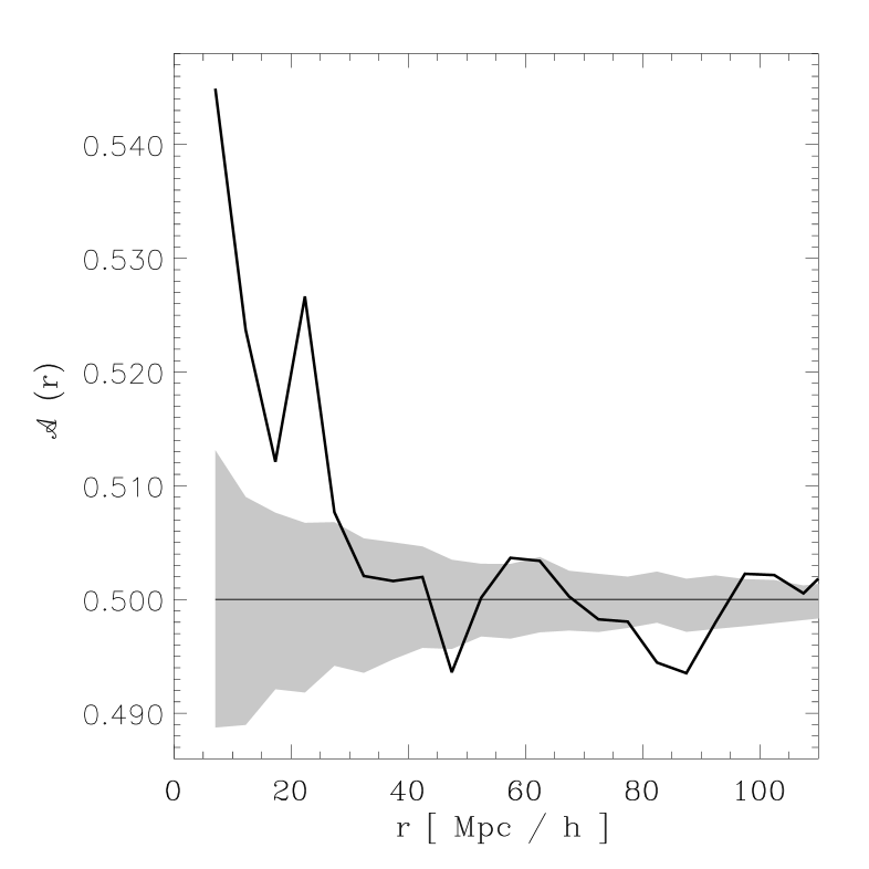
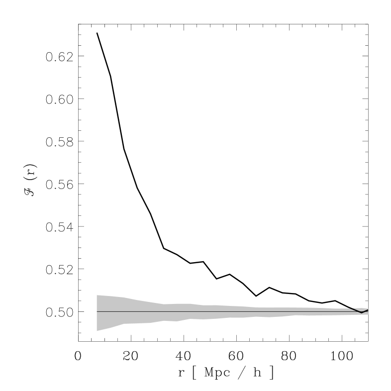
In the following we will use the direction of the major axis of the mass ellipsoid (the “$a$-axis”) as a vector mark ${\mathbf{l}}$. Fig. 3 shows the mark correlation functions ${\cal A}(r)$ and ${\cal F}(r)$. The increased ${\cal A}(r)$ towards smaller scales indicates that pairs of clusters with a distance smaller than 30 $h^{-1}$Mpc prefer a parallel orientation of their orientation axes ${\mathbf{l}}_{1}$ and ${\mathbf{l}}_{2}$. This deviation of $\sim 10\%$ from the signal of a purely random orientation is clearly outside the random fluctuations shown by the shaded region. We determine these random fluctuations by repeatedly and randomly redistributing the orientation axes among the clusters. The positions of the clusters remain fixed. The filamentary alignment of the orientation of the clusters ${\mathbf{l}}_{1}$ and ${\mathbf{l}}_{2}$ towards the connecting vector $\hat{\mathbf{r}}$ as quantified by ${\cal F}(r)$ is significantly stronger (up to 20% deviation from the signal of purely random orientation on small scales). Remarkably this signal extends out to 100 $h^{-1}$Mpc. In a qualitative picture this may be explained by a large number of clusters elongated in the direction of the filaments of the large scale structures. Filaments are prominent features found in the observed galaxy distribution (Huchra et al., 1990) as well as in $N$-body simulations (Melott & Shandarin, 1990), often with an extent up to 100 $h^{-1}$Mpc. The inspection of density field of the simulation utilized here confirms this view (see Fig. 5).

Figure 3: Mark correlations using the 3D orientation of the dark matter halo, specified by the direction of the major axis ${\mathbf{l}}$ of the mass ellipsoid, as vector mark. The shaded area is obtained by randomizing the orientation among the clusters.

Up to now we used the orientation of the mass ellipsoid in three dimensional space. Most observations, however, only provide the projected galaxy number density or X-ray intensity. In the following we will investigate whether the clear signal found in Fig. 3 will be reduced by projection. In close analogy to our three dimensional analysis we determine the orientation of the mass-ellipse of a halo from the mass-density orthogonally projected onto a side of the simulation box. We repeat our analysis with the major axis of the mass ellipse in two-dimensions as a two-dimensional vector mark. Also the normalized direction $\hat{\mathbf{r}}$ is given in the plane. However, for the radial distance $r$ we use the three dimensional separation of the clusters. With this setting, we mimic the observational constraints, e.g. in the Reflex cluster survey. In this projected sample the signal in ${\cal A}(r)$ is only visible on scales smaller than 10 $h^{-1}$Mpc (Fig. 4). The amplitude of the deviation from random orientation (in two dimension $2/\pi$) is reduced, as well. But still, the filamentary alignment quantified with ${\cal F}(r)$ indicates a strong alignment of the orientation of the clusters with the connecting vector (Fig. 4). Although the amplitude is slightly reduced, this alignment is still visible out to scales of 100 $h^{-1}$Mpc, as in the three dimensional analysis.

Figure 4: Mark correlations with the normalized major axis $|{\mathbf{l}}|=1$ of the projected cluster-density (2D orientation) as vector mark. The shaded area is obtained by randomizing the orientation among the clusters.

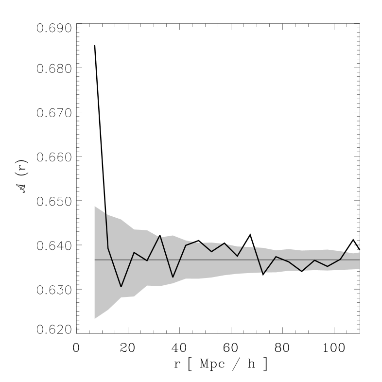
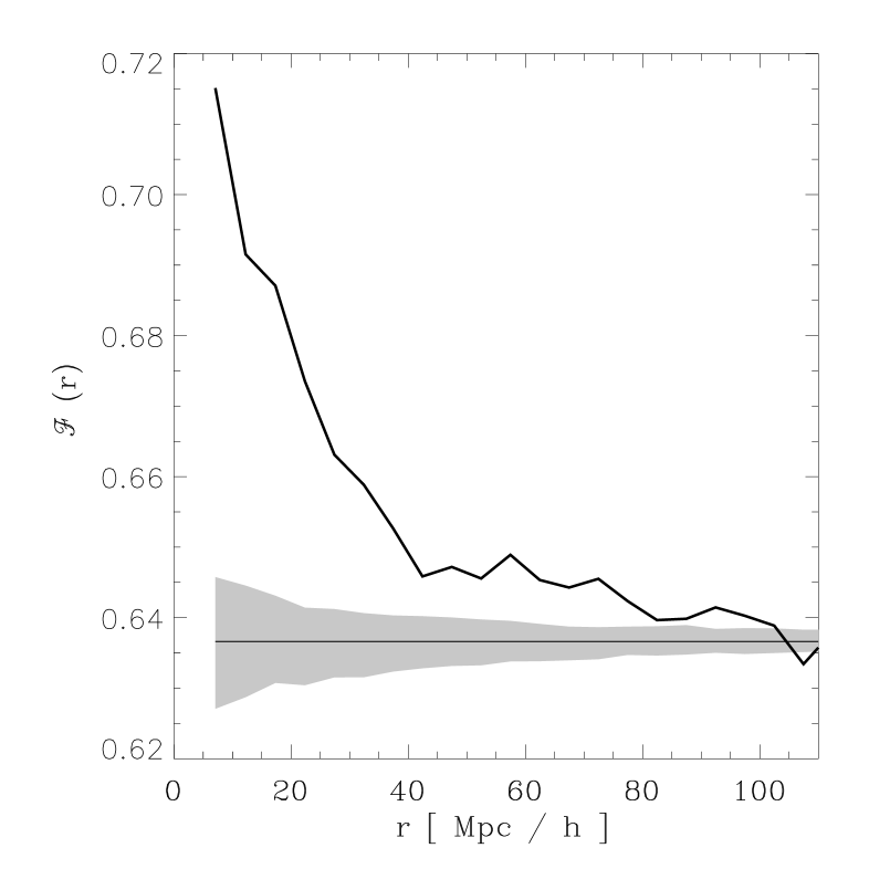
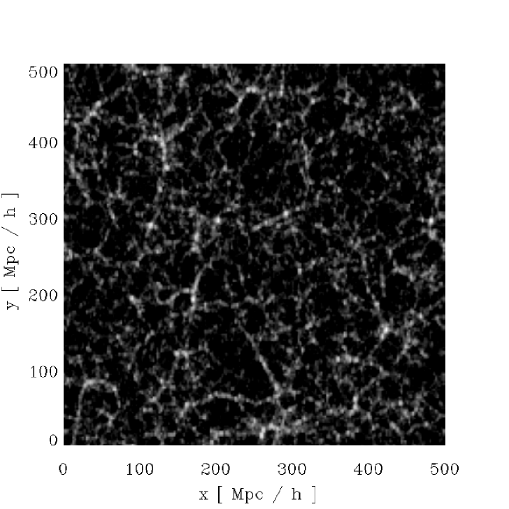
The question arises, why do we find two different regimes of the vector correlations, using either ${\cal A}(r)$ or ${\cal F}(r)$. The direct alignment, quantified with ${\cal A}(r)$ extends out to 30 $h^{-1}$Mpc, whereas the filamentary alignment (${\cal F}(r)$) is visible out to 100 $h^{-1}$Mpc. A glimpse on the real density distribution in Fig. 5 sheds light on this topic. Clearly one can see filamentary structures with sizes extending up to $100\leavevmode\nobreak\ {{h^{-1}{\rm Mpc}}}$, for example the two pronounced filaments which end up in the knot at $x\approx 275\leavevmode\nobreak\ {{h^{-1}{\rm Mpc}}}$ and $y\approx 75\leavevmode\nobreak\ {{h^{-1}{\rm Mpc}}}$. Generically, such filaments are not straight but crinkled and show a lot of small branches. This implies that the coherence of the angles between the major axes of clusters harbored in these filamentary structures is lost soon. Consequently the positive correlation seen with ${\cal A}(r)$ is confined to comparatively small scales $\lesssim 30\leavevmode\nobreak\ {{h^{-1}{\rm Mpc}}}$s (in the case of projected data even to $\lesssim 10\leavevmode\nobreak\ {{h^{-1}{\rm Mpc}}}$). On the other hand, the signal exploring the angle between orientation and connecting vector is not affected by the small scale disorder. Thus ${\cal F}(r)$ is tracing the filamentary alignment out to scales of 100 $h^{-1}$Mpc.

Figure 5: Projected density field of a $\sim 7.5\leavevmode\nobreak\ {{h^{-1}{\rm Mpc}}}$ slice through the simulation box. The density is calculated on a $300^{3}$ grid which corresponds to a smoothing length of $\sim 1.7\leavevmode\nobreak\ {{h^{-1}{\rm Mpc}}}$. The maximum value of projected density is $\approx 1.5\times 10^{4}\rho/\rho_{\rm mean}$. Gray scales are chosen according to $\log$ of density.

5 Angular momentum, mass and spin correlations

In a simulation we have access to the position and the velocity of the particles. Hence, it is easy to determine the angular momenta of our cluster sized halos. In this section we use the direction of the angular momenta of galaxy clusters as vector marks and compare their correlation properties with the alignment seen in the orientation of the mass distribution (Sect. 4). With scalar MCFs, using the absolute value of the angular momentum, the cluster mass and the spin parameter as scalar mark, we will supplement the foregoing result.

It is well known that there exists a correlation between the axes of the mass ellipsoid and the direction of the angular momentum in gravitationally bound N-body systems (Binney & Tremaine, 1987). Fig. 6 shows that the major axis of the mass ellipsoid tends to be perpendicular to the angular momentum. Compared to the expectation from a purely random distribution, the minor axis favors smaller angles with the angular momentum.

Figure 6: Cumulative plot of the number of clusters and the cosine between the direction of the angular momentum and the major, medium and minor cluster axis, respectively.

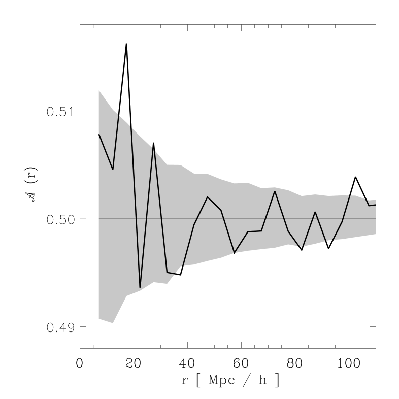
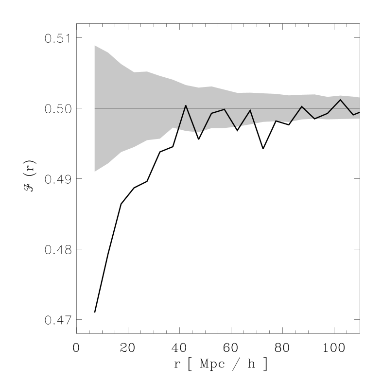
Hence, using the direction of the angular momentum as vector mark, we are expecting to see effects comparable to the shape orientations. The vector correlations of the directions of the angular momentum are shown in Fig. 7. There is no clear signal for a direct alignment of the angular momenta as traced by ${\cal A}(r)$. However, the correlation ${\cal F}(r)<0.5$ is smaller than for random directions (shaded area), this indicates that the angular momenta are preferably oriented perpendicular to the connecting vector $\hat{\mathbf{r}}$ on scales up to $30\leavevmode\nobreak\ {{h^{-1}{\rm Mpc}}}$. The amplitude of the deviation from the random orientation reaches approximately 5% and is clearly outside the fluctuations. With Fig. 6 in mind, the latter result was expected from the correlations of the orientations shown in Fig. 3: For a pair of clusters residing in a filamentary structure the connecting vector is oriented along this filament. The major axes of the orientations tend to align with the filaments, and therefore the angular momenta tend to stand perpendicular to the filaments. A random orientation of the angular momenta in the planes perpendicular to the filaments provides a simple explanation for the absence of any signal in ${\cal A}(r)$, still compatible with the strong signal in ${\cal F}(r)$.

Figure 7: Mark correlation functions using the normalized angular momentum ${\mathbf{l}}$ with $|{\mathbf{l}}|=1$ as vector mark. The shaded area is obtained by randomizing the orientation among the clusters.

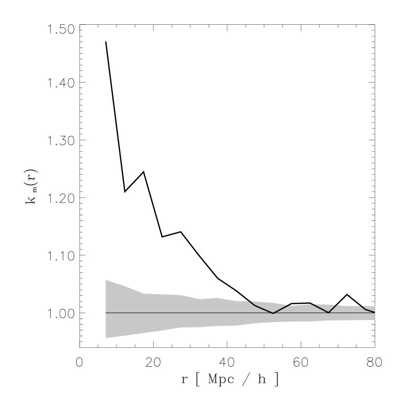
Besides the correlations in the directions of the angular momentum vectors, we are also interested in the correlations of their magnitudes. We investigate these correlations with the MCFs discussed in Sect. 3.1, using the magnitude of the angular momentum as a scalar mark. In Fig. 8 the increased $k_{\rm m}(r)$ shows that pairs of clusters with separations $\lesssim 50\leavevmode\nobreak\ {{h^{-1}{\rm Mpc}}}$ tend to have higher mean angular momentum compared to the overall mean angular momentum. The positive covariance up to $\lesssim 15\leavevmode\nobreak\ {{h^{-1}{\rm Mpc}}}$ indicates that both members of close pairs tend to have similar angular momentum. Hence, inspecting both $k_{\rm m}$ and the covariance, we see that close clusters tend to carry a similar amount of angular momentum, larger than the overall mean angular momentum.

Figure 8: Mark correlation functions with the absolute value of the angular momentum of the cluster as scalar mark. The shaded area is obtained by randomizing the mark among the clusters.

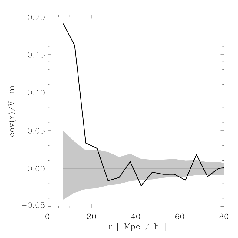
There are two possibilities to explain this behavior. On the one hand the mean mass of a close cluster pair could be enhanced, and so the absolute value of the angular momentum would grow simply due to the fact that bigger clusters are under consideration. Indeed, Gottlöber et al. (2002) found such an increase in the mean mass in close pairs (in their case traced by the maximum circular velocity of the halo). Consistently Beisbart & Kerscher (2000) report an enhanced luminosity for close galaxy pairs. On the other hand, the rotational support of close cluster pairs could be higher, meaning that the spin parameter $\lambda$ is enhanced, cp. Eq. (1). To illustrate this further, we investigate the MCFs with the mass and the spin parameter as marks:
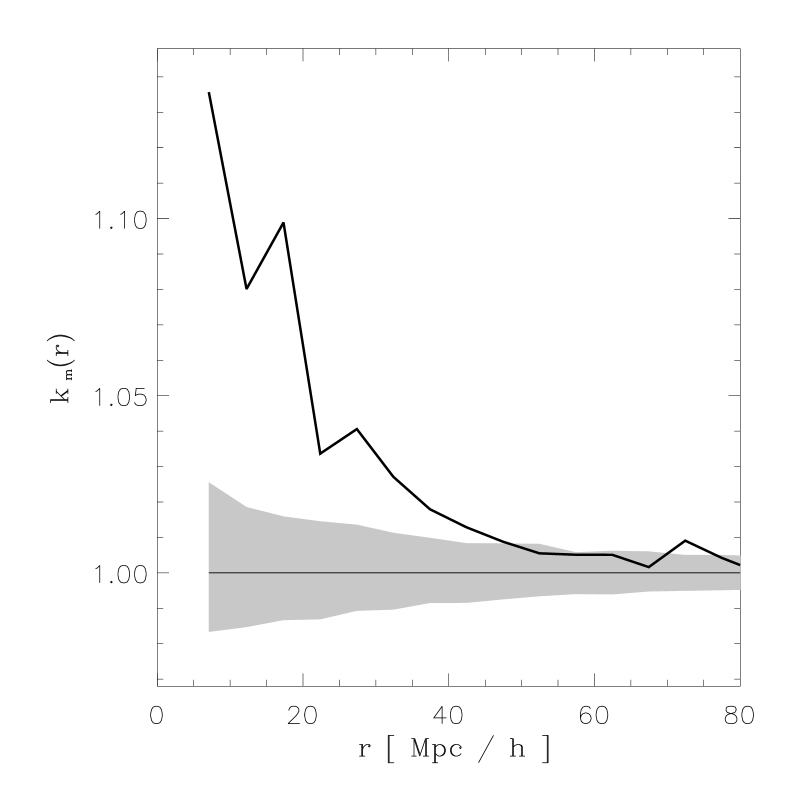
Mass: In Fig. 9 we show the MCFs of the cluster distribution with the total mass as scalar mark. The increased $k_{\rm m}(r)$ indicates that close pairs of clusters tend to have higher mean masses than the overall mean mass $\overline{m}$ on scales out to 50 $h^{-1}$Mpc. The signal shows a deviation up to 10% from a purely random distribution. The conditional covariance ${{\text{{\em cov}}}}(r)$ shows only a weak positive signal, confined to scales below 15 $h^{-1}$Mpc, indicating that only close pairs tend to have similar masses.

Figure 9: Mark correlation functions with the mass of the cluster halo as scalar mark. The shaded area is obtained by randomizing the mark among the cluster halos.

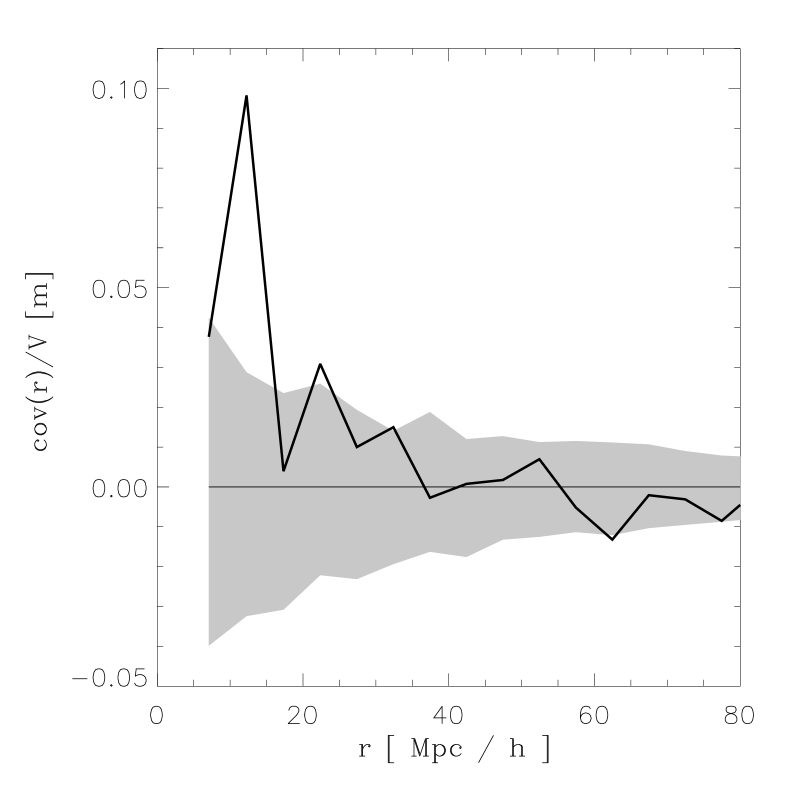
Spin: In Fig. 10 we show the MCFs of the cluster distribution with the spin parameter $\lambda$ as scalar mark. The increased $k_{\rm m}(r)$ indicates that neighboring pairs of clusters tend to have higher spin parameter $\lambda$ compared to the overall mean spin $\overline{\lambda}$. The signal seen in Fig. 10 shows an enlarged spin parameter of clusters on scales out to 50 $h^{-1}$Mpc, the same range as for the mass. The deviation from random distribution is $\sim 15\%$. Hence, not only an increased mass accretion but also tidal interactions out to fairly large scales seem to characterize the regions around cluster halos. The conditional covariance ${{\text{{\em cov}}}}(r)$ shows no signal. This can be explained by looking at the mark variance ${{\text{{\em var}}}}(r)$. The signal at small distances deviates about $50\%$ from random, indicating large scattering of the spin parameter. This large dispersion also might be the reason why previous studies did not find an environmental dependence of the amount of the spin parameter. A sufficiently large simulation and also a large number of clusters are needed to get a clear signal in the MCFs for the spin parameter.

Figure 10: Mark correlation function with the spin parameter $\lambda$ of the cluster halo as scalar mark. The shaded area is obtained by randomizing the mark among the clusters.

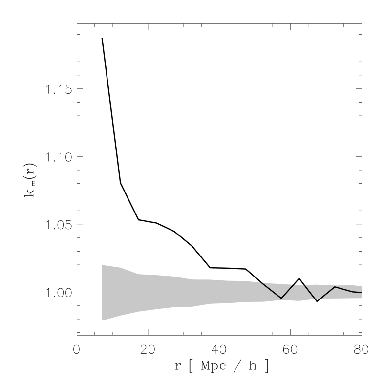
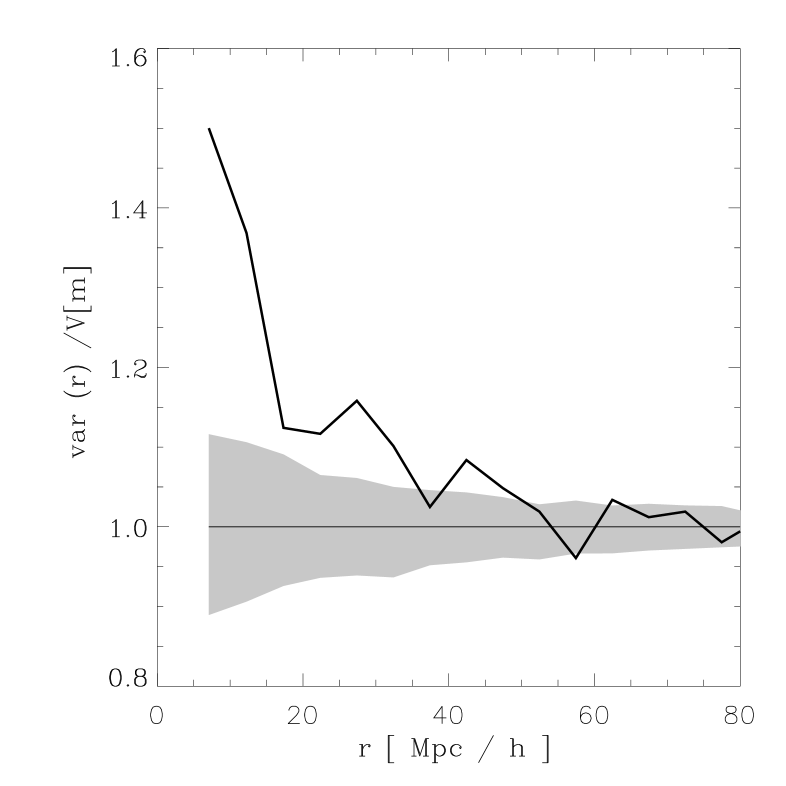
Putting together all the results shown in Figs. 8 -10, it turns out that the increased mean angular momentum is not only caused by an enhanced mass, but also by an enlarged spin parameter of neighboring pairs of clusters. From the present analysis we can not draw any firm conclusions, whether this phenomenon is dominated by tidal interaction or merging processes. There are compelling observational hints (see e.g. Plionis & Basilakos 2002; Schuecker et al. 2001) that clusters in high-density environments show indications of dynamical disruption. Thus it seems to be likely that the enhancement of the angular momentum of close neighbors is caused by a substantial mass accretion (i.e. merging). The concordant behavior of the mass and the spin MCF support this interpretation, at least on scales below $\sim 15\leavevmode\nobreak\ {{h^{-1}{\rm Mpc}}}$. However, tidal interactions could be the cause for the correlations seen on large scales.

6 Summary

Whether there exist correlations in the orientations of galaxies or galaxy clusters has been discussed for a long time. Binggeli (1982) reported a significant alignment of the observed galaxy clusters out to 50 $h^{-1}$Mpc. Struble & Peebles (1985, 1986) claimed that this effect is small and prone to systematics and Ulmer et al. (1989) find no indication in their investigation. Subsequently, several authors found, sometimes only weak, signs of alignments in the galaxy and galaxy cluster distribution (see e.g. Djorgovski 1986; Lambas et al. 1988; Fuller et al. 1999; Heavens et al. 2000). As a novel statistical method we have used the mark correlation functions (MCFs) to quantify the alignment of cluster sized halos, extracted from a large scale simulation based on a $\Lambda$CDM cosmology. Our sample with 3000 cluster sized halos is bigger than the currently available samples of galaxy clusters. The unambiguous signal we obtain benefits from the large statistics in our simulation.

Using two different weighting functions in the construction of the MCFs we investigate the direct alignment and the filamentary alignment. First we use the major axis of the mass ellipsoid as our direction marker. The clear signal from the direct alignment ${\cal A}(r)$ extends out $\sim 30\leavevmode\nobreak\ {{h^{-1}{\rm Mpc}}}$. For the filamentary alignment ${\cal F}(r)$ we find deviations from isotropy up to $\sim 100\leavevmode\nobreak\ {{h^{-1}{\rm Mpc}}}$. Considering the projected mass distribution, the signal from the direct alignment ${\cal A}(r)$ already vanishes at a scale of $\sim 10\leavevmode\nobreak\ {{h^{-1}{\rm Mpc}}}$. However, we find a filamentary alignment ${\cal F}(r)$ out to scales of $\sim 100\leavevmode\nobreak\ {{h^{-1}{\rm Mpc}}}$, even for the projected data. This scale is very similar to the size of the large scale filaments seen in our simulation. We think that the function ${\cal F}(r)$ is a powerful tool for exploring large scale alignment effects also in observational data.

Franx et al. (1991) showed that the angular momentum of an ellipsoidal system tends to align with the minor axis of this system. We confirm this behavior in our simulation. With the angular momentum as vector mark, ${\cal F}(r)$ shows the expected filamentary correlations: the angular momentum tends to be perpendicular to the connecting line, i.e. the filament, up to separations of $\sim 40\leavevmode\nobreak\ {{h^{-1}{\rm Mpc}}}$. However, we obtain no signal for the direct alignment ${\cal A}(r)$. This is in concordance with the perception that the angular momenta are randomly oriented in the planes perpendicular to the filaments.

With the scalar MCFs $k_{\rm m}(r)$ and ${{\text{{\em cov}}}}(r)$ we have investigated the correlations in the absolute value of the angular momentum. Close pairs of clusters tend to have similar and also higher absolute values of the angular momentum compared to the global average. A clear signal can be detected up to $\sim 50\leavevmode\nobreak\ {{h^{-1}{\rm Mpc}}}$. A further analysis of the mass and spin parameter distribution of the clusters with the MCFs has shown that this enhancement of the absolute value of the angular momentum is caused by an enhanced mass of close pairs of clusters as well as by the stronger rotational support of them. This behavior should be caused by the combined action of large-scale tidal fields and the hierarchical merging of progenitor structures and mass inflow onto the cluster. Since this mass growth follows the large scale filaments, tidal interactions and merger events are tightly connected. The mark correlation function with scalar and vector marks deliver quantitative measures of these effects.

Acknowledgments

M.K. was supported by the Sonderforschungsbereich 375 für Astro–Teilchenphysik der Deutschen Forschungsgemeinschaft.

References

- Beisbart & Kerscher (2000) Beisbart, C. & Kerscher, M. 2000, ApJ, 545, 6
- Beisbart et al. (2002) Beisbart, C., Kerscher, M., & Mecke, K. 2002, to appear in: Lecture Notes in Physics, second Wuppertal conference ”Spatial statistics and statistical physics”, physics/0201069
- Binggeli (1982) Binggeli, B. 1982, A&A, 107, 338
- Binney & Silk (1979) Binney, J. & Silk, J. 1979, MNRAS, 188, 273
- Binney & Tremaine (1987) Binney, J. & Tremaine, S. 1987, Galactic dynamics (Princeton, NJ, Princeton University Press, 1987, 747 p.)
- Böhringer et al. (1998) Böhringer, H., Guzzo, L., Collins, C., et al. 1998, ESO Messenger, 21
- Chambers et al. (2000) Chambers, S., Melott, A., & Miller, C. 2000, ApJ, 544, 104
- Colberg et al. (2000) Colberg, J. M., White, S. D. M., Yoshida, N., et al. 2000, MNRAS, 319, 209
- Cole & Lacey (1996) Cole, S. & Lacey, C. 1996, MNRAS, 281, 716
- Collins et al. (2000) Collins, C., Guzzo, L., Böhringer, H., et al. 2000, MNRAS, 319, 939
- Cooray (2000) Cooray, A. R. 2000, MNRAS, 313, 783
- Couchman (1991) Couchman, H. 1991, ApJ, 368, L23
- Cressie (1991) Cressie, N. 1991, Statistics for spatial Data (Chichester: John Wiley & Sons)
- Djorgovski (1986) Djorgovski, S. 1986, in Nearly Normal Galaxies, ed. S. M. Faber, 225
- Doroshkevich (1973) Doroshkevich, A. G. 1973, ApJ, 14, 11
- Flin (1987) Flin, P. 1987, MNRAS, 228, 941
- Fong et al. (1990) Fong, R., Stevenson, P., & Shanks, T. 1990, MNRAS, 242, 146
- Franx et al. (1991) Franx, M., Illingworth, G., & de Zeeuw, T. 1991, ApJ, 383, 112
- Fuller et al. (1999) Fuller, T. M., West, M. J., & Bridges, T. J. 1999, ApJ, 519, 22
- Gottlöber et al. (2002) Gottlöber, S., Kerscher, M., Kravtsov, A., Faltenbacher, A., & Müller, V. 2002, A&A, in press, astro-ph/0203148
- Gottlöber et al. (2001) Gottlöber, S., Klypin, A. A., & Kravtsov, A. V. 2001, ApJ, 546, 223
- Heavens et al. (2000) Heavens, A. F., Refregier, A., & Heymans, C. 2000, MNRAS, 319, 649
- Huchra et al. (1990) Huchra, J. P., Geller, M. J., De Lapparent, V., & Corwin Jr., H. G. 1990, ApJS, 72, 433
- Katgert et al. (1996) Katgert, P., Mazure, A., Perea, J., et al. 1996, A&A, 310, 8
- Kitayama & Suto (1996) Kitayama, T. & Suto, Y. 1996, ApJ, 469, 480
- Knebe et al. (2000) Knebe, A., Kravtsov, A. V., Gottlöber, S., & Klypin, A. A. 2000, MNRAS, 317, 630
- Knebe & Müller (1999) Knebe, A. & Müller, V. 1999, A&A, 341, 1
- Lambas et al. (1988) Lambas, D. G., Groth, E. J., & Peebles, P. 1988, AJ, 95, 975
- Martin et al. (1995) Martin, D., Nichol, R., Collins, C., Lumsden, S., & Guzzo, L. 1995, MNRAS, 274, 623
- Melott & Shandarin (1990) Melott, A. L. & Shandarin, S. F. 1990, Nature, 346, 633
- Onuora & Thomas (2000) Onuora, L. I. & Thomas, P. A. 2000, MNRAS, 319, 614
- Padmanabhan (1993) Padmanabhan, T. 1993, Structure formation in the Universe (Cambridge: Cambridge University Press)
- Plionis (1994) Plionis, M. 1994, ApJS, 95, 401
- Plionis & Basilakos (2002) Plionis, M. & Basilakos, S. 2002, MNRAS, 329, L47
- Porciani et al. (2002a) Porciani, C., Dekel, A., & Hoffman, Y. 2002a, ApJ, 332, 325
- Porciani et al. (2002b) —. 2002b, ApJ, 332, 339
- Rhee & Katgert (1987) Rhee, G. & Katgert, P. 1987, A&A, 183, 217
- Rhee & Latour (1991) Rhee, G. & Latour, H. 1991, A&A, 243, 38
- Schuecker et al. (2001) Schuecker, P., Böhringer, H., Reiprich, T. H., & Feretti, L. 2001, AA, 378, 408
- Seljak & Zaldarriaga (1996) Seljak, U. & Zaldarriaga, M. 1996, ApJ, 469, 437
- Stoyan (1984) Stoyan, D. 1984, Math. Nachr., 116, 197
- Stoyan & Stoyan (1994) Stoyan, D. & Stoyan, H. 1994, Fractals, Random Shapes and Point Fields (Chichester: John Wiley & Sons)
- Struble & Peebles (1985) Struble, M. F. & Peebles, P. 1985, AJ, 90, 582
- Struble & Peebles (1986) —. 1986, AJ, 91, 1474
- Szapudi et al. (2000) Szapudi, I., Branchini, E., Frenk, C., Maddox, S., & Saunders, W. 2000, MNRAS, 318, L45
- Ulmer et al. (1989) Ulmer, M., McMillan, S. L. W., & Kowalski, M. P. 1989, ApJ, 338, 711
- van Haarlem et al. (1997) van Haarlem, M. P., Frenk, C. S., & White, S. D. M. 1997, MNRAS, 287, 817
- Vitvitska et al. (2001) Vitvitska, M., Klypin, A., Kravtsov, A., et al. 2001, astro-ph/0105349
- West (1994) West, M. J. 1994, MNRAS, 268, 79
- White (1984) White, S. D. M. 1984, ApJ, 286, 38