Similarities and Differences between Relativistic Electron-Photon Cascades Developed in Matter, Photon Gas and Magnetic Field

Abstract

We investigate the properties of astrophysical electromagnetic cascades in matter, photon gas and magnetic fields, and discuss similarities and differences between characteristics of electron-photon showers developed in these 3 substances. We apply the same computational technique based on solution of the adjoint cascade equations to all 3 types of cascades, and present precise numerical calculations of cascade curves and broad-band energy spectra of secondary electrons and photons at different penetration lengths.

1 Introduction

Relativistic electrons – directly accelerated, or being secondary products of various hadronic processes – may result in copious $\gamma$-ray production caused by interactions with ambient targets in forms of gas (plasma), radiation and magnetic fields. In different astrophysical environments $\gamma$-ray production may proceed with high efficiency through bremsstrahlung, inverse Compton scattering and synchrotron (and/or curvature) radiation, respectively. Generally, $\gamma$-ray production is effective when the cooling time that characterizes the rate of the process does not significantly exceed (i) the source (accelerator) age (ii) the characteristic time of non-radiative losses caused by adiabatic expansion of the source or particle escape and (iii) the cooling time of competing radiation mechanisms that result in low-energy photons outside the $\gamma$-ray domain. As long as the charged particles are effectively confined in the $\gamma$-ray production region, at some circumstances these condition could be fulfilled even in environments with a relatively low gas and photon densities or weak magnetic field. More specifically, the $\gamma$-ray production efficiency could be close to 1 even when $t_{\rm rad}\gg R/c$ ($R$ is the characteristic linear size of the production region, $c$ is the speed of light). In such cases the secondary $\gamma$-rays escape the source without significant internal absorption. Each of the above mentioned $\gamma$-ray production mechanisms has its major “counterpart” - $\gamma$-ray absorption mechanism of same electromagnetic origin resulting in electron-positron pair production in matter (the counterpart of bremsstrahlung), in photon gas (the counterpart of inverse Compton scattering), and in magnetic field (the counterpart of synchrotron radiation). The $\gamma$-ray production mechanisms and their absorption counterparts have similar cross-sections, therefore the condition for radiation $t_{\rm rad}\geq R/c$ generally implies small optical depth for the corresponding $\gamma$-ray absorption mechanism, $\tau_{\rm abs}\leq 1$. But in many astrophysical scenarios, in particular in compact galactic and extragalactic objects with favorable conditions for particle acceleration, the radiation processes proceed so fast that $t_{\rm rad}\geq R/c$. At these conditions the internal $\gamma$-ray absorption becomes unavoidable. If the $\gamma$-ray production and absorption processes occur in relativistic regime, namely when (i) $E_{\rm\gamma,e}\geq 10^{3}m_{e}c^{2}$ in the hydrogen gas, (ii) $E_{\rm\gamma,e}\epsilon\gg m_{\rm e}^{2}c^{4}$ in photon gas (often called Klein-Nishina regime; $\epsilon$ is the average energy of the target photons), or (iii) $(E_{\rm\gamma,e}/m_{\rm e}c^{2})(H/H_{\rm cr})\gg 1$ in the magnetic field (often called quantum regime; $H_{\rm cr}\simeq 4.4\times 10^{13}\ \rm G$ is the so-called critical strength of the magnetic field), the problem cannot be reduced to a simple absorption effect. In this regime, the secondary electrons produce new generation of high energy $\gamma$-rays, these photons again produce electron-positron pairs, so the electromagnetic cascade develops.

The characteristics of electromagnetic cascades in matter have been comprehensively studied, basically in the context of interactions of cosmic rays with the Earth’s atmosphere (see e.g. [1]) as well as for calculations of performance of detectors of high energy particles (e.g. [2]). The theory of electromagnetic cascades in matter can be applied to some sources of high energy cosmic radiation, in particular to the “hidden source” scenarios like massive black holes in centers of AGN or young pulsars inside the dense shells of recent supernovae explosions (see e.g. [3]). Within another, so-called “beam dump” models (see e.g. Ref. [3, 5]) applied to X-ray binaries, protons accelerated by the compact object (a neutron star or black hole), hit the atmosphere of the normal companion star, and thus result in production of high energy neutrinos and $\gamma$-rays [4]. In such objects, the thickness of the surrounding gas can significantly exceed $100\ \rm g/cm^{2}$, thus the protons produced in the central source would initiate (through production of high energy $\gamma$-rays and electrons) electromagnetic showers. These sources perhaps represent the “best hope” of neutrino astronomy, but they are generally considered as less attractive targets for gamma-ray astronomy. However, the $\gamma$-ray emission in these objects is not fully suppressed. The recycled radiation with spectral features determined by the thickness (“grammage”) of the gas shell, should be seen in $\gamma$-rays in any case, unless the synchrotron radiation of secondary electrons dominates over the bremsstrahlung losses and channels the main fraction of the nonthermal energy into the sub gamma-ray domains.

The development of electromagnetic cascades in photon gas and magnetic fields is a more common phenomenon in astrophysics. In photon fields such cascades can be created on almost all astronomical scales, from compact objects like accreting black holes [6, 7, 8, 9, 10], fireballs in gamma-ray bursts [11] and sub-pc jets of blazars [12] to large-scale (up to $\geq 100$ kpc) AGN jets [13, 14] and $\geq 1$ Mpc size clusters of galaxies [15]. Electromagnetic cascades in the intergalactic medium lead to formation of huge ($\geq 10$ Mpc) nonthermal structures like hypothetical electron-positron pair halos [16]. Finally, there is little doubt that the entire Universe is a scene of continuous creation and development of electromagnetic cascades. All $\gamma$-rays  of energy $\geq$ a few GeV emitted by astrophysical objects have a similar fate. Sooner or later they terminate on Hubble scales due to interactions with the diffuse extragalactic background. Since the energy density of 2.7 K CMBR significantly exceeds the energy density of intergalactic magnetic fields, these interactions initiate electron-photon cascades [17]. The superposition of contributions of $\gamma$-rays  from these cascades should constitute a significant fraction of the observed diffuse extragalactic background.

Bonometto and Rees [18] perhaps where the first who realized the astrophysical importance of development of electron-photon cascades supported by $\gamma$-$\gamma$ pair-production and inverse Compton scattering in dense photon fields. When the so called compactness parameter [19] $l=(L/R)(\sigma_{\rm T}/m_{\rm e}c^{3})$ (L is the luminosity and R is the radius of the source) is less than 10, then the cascade is developed in the linear regime, i.e. when the soft radiation produced by cascade electrons do not have a significant feedback effect on the cascade development. In many cases, including the cascade development in compact objects, this approximation works quite well.

The first quantitative study of characteristic of linear cascades in photon fields has been performed using the method of Monte Carlo simulations [20]. Generally, the kinetic equations for the cascade particles can be solved only numerically. However, with some simplifications it is possible to derive useful analytical approximations [7, 8] which help to understand the features of the steady-state solutions for cascades in photon fields.

The cascade development in the magnetic field is a key element to understand the physics of pulsar magnetospheres [21, 22], therefore it is generally treated as a process associated with very strong magnetic fields. However, such cascades could be triggered in many other (at first glance unusual) sites like the Earth’s geomagnetic field [23, 24, 25], accretion disks of massive black holes [26], etc. In general, the pair cascades in magnetic fields are effective when the product of the particle (photon or electron) energy and the strength of the field becomes close to the “quantum threshold” of about $H_{\rm crit}m_{\rm e}c^{2}\simeq 2\times 10^{7}\ \rm TeV\cdot G$, unless we assume a specific, regular field configuration. An approximate approach, similar to the so-called approximation A of cascade development in matter [1], has been recently applied by Akhiezer et al. [27]. Although this theory quite satisfactorily describes the basic features of photon-electron showers, it does not provide an adequate accuracy for quantitative description of the cascade characteristics [24]. Note that in both studies approximate cross-sections for magnetic bremsstrahlung and magnetic pair-production have been used, thus reducing the validity of the results to the limit $EH\gg 10^{7}\ \rm TeV\cdot G$ ($E$ is the minimum energy of secondary particles being under consideration).

As long as we are interested in the one-dimensional cascade development (which seems to be quite sufficient for many astrophysical purposes), all 3 types of cascades can be described by the same integro-differential equations like the ones derived by Landau and Rumer [28], but in each case specifying the cross-sections of relevant interaction processes. The solution of these equations in a broad range of energies is however not a trivial task. In this paper we present the results of our recent study of cascade characteristics in 3 substances - matter, photon gas and magnetic field - with emphasis on the analysis of similarities and differences between these 3 types of cascades. For quantitative studies of these characteristics we have chosen the so-called technique of adjoint cascade equations. Although this work has been initially motivated by methodological and pedagogical objectives, some results are rather original and may present practical interest in certain areas of high energy astrophysics.

2 Technique of adjoint cascade equations

The results of this study are based on numerical solutions of the so-called adjoint cascade equations. The potential of this computational technique, in particular its possible applications to different problems of cosmic ray physics has been comprehensively described in Ref.[29]. Below we briefly discuss the main features of solution of the adjoint cascade equations. For our purposes it is quite sufficient to consider only the longitudinal development of electromagnetic cascades neglecting the emission angles of secondary particles and, thus, assuming that all cascade particles are moved along the shower axis. Besides, we neglect the differences in interactions of electrons and positrons, i.e. do not consider positron annihilation, both in flight and after thermalization in the ambient plasma. This is a quite good approximation as long as we are interested in $\gamma$-ray energies exceeding $\alpha_{\rm f}^{-1}m_{\rm e}c^{2}\simeq 70\ \rm MeV$ ($\alpha_{\rm f}=1/137$ is the fine structure constant). Under these assumptions, the system of adjoint cascade equations reads

$$\frac{\partial f}{\partial t}+f/\lambda_{e}-\int_{\varepsilon_{th}}^{\varepsilon}W_{ee}(\varepsilon,\varepsilon^{\prime})f(t,\varepsilon^{\prime})d\varepsilon^{\prime}-\int_{\varepsilon_{th}}^{\varepsilon}W_{e\gamma}(\varepsilon,\varepsilon^{\prime})g(t,\varepsilon^{\prime})d\varepsilon^{\prime}=F(t,\varepsilon),$$ (1)

$$\frac{\partial g}{\partial t}+g/\lambda_{\gamma}-\int_{\varepsilon_{th}}^{\varepsilon}W_{\gamma e}(\varepsilon,\varepsilon^{\prime})f(t,\varepsilon^{\prime})d\varepsilon^{\prime}-\int_{\varepsilon_{th}}^{\varepsilon}W_{\gamma\gamma}(\varepsilon,\varepsilon^{\prime})g(t,\varepsilon^{\prime})d\varepsilon^{\prime}=G(t,\varepsilon).$$ (2)

The adjoint functions $f(t,\varepsilon)$ and $g(t,\varepsilon)$ in Eqs. (1) and (2) describe the contributions (averaged over random realizations of the cascade development) from cascade initiated by a primary electron ($f$) or a photon ($g$) of energy $\varepsilon$ (all energies are expressed in units $m_{e}c^{2}$); $t$ is the cascade penetration depth; $\varepsilon_{th}$ is the minimum energy of cascade particles being under consideration.

The parameter $\lambda_{\alpha}$ in Eqs. (1) and (2) defines the mean free path length of cascade particles of type $\alpha$ ($\alpha=e\ \rm or\ \gamma$). It can be expressed through the total cross-sections ($\sigma_{\alpha}$) of interaction with the ambient medium. In the most general case, when the medium consists of matter ($M$), magnetic field ($F$) and photon gas ($G$),

$$\lambda_{\alpha}=\left[n_{0}^{(M)}\sigma_{\alpha}^{(M)}+\sigma_{\alpha}^{(F)}+n_{0}^{(G)}\sigma_{\alpha}^{(G)}\right]^{-1}$$ (3)

where $n_{0}^{(M)}$ and $n_{0}^{(F)}$ are the number density of the matter atoms and the ambient photons, respectively. The parameters

$$W_{\alpha\beta}(\varepsilon,\varepsilon^{\prime})=n_{0}^{(M)}w_{\alpha\beta}^{(M)}(\varepsilon,\varepsilon^{\prime})+w_{\alpha\beta}^{(F)}(\varepsilon,\varepsilon^{\prime})+n_{0}^{(G)}w_{\alpha\beta}^{(G)}(\varepsilon,\varepsilon^{\prime})$$ (4)

are differential cross-sections over the energy $\varepsilon^{\prime}$ of the secondary particle of type $\beta$ ($\beta=e$ or $\gamma$). They are normalized as

$$\int W_{\alpha\beta}(\varepsilon,\varepsilon^{\prime})d\varepsilon^{\prime}=n_{0}^{(M)}\bar{n}_{\alpha\beta}^{(M)}\sigma_{\alpha}^{(M)}+\bar{n}_{\alpha\beta}^{(F)}\sigma_{\alpha}^{(F)}+n_{0}^{(G)}\bar{n}_{\alpha\beta}^{(G)}\sigma_{\alpha}^{(G)}$$ (5)

where $\bar{n}_{\alpha\beta}^{(M)}$, $\bar{n}_{\alpha\beta}^{(F)}$ and $\bar{n}_{\alpha\beta}^{(G)}$ are the mean multiplicities of secondary particles of type $\beta$ produced by a particle of type $\alpha$.

Properties of the particle “detector” located at the depth $t$ are defined by the right hand side functions $F$ and $G$ in Eqs.  (1) and (2) and by the boundary conditions $f(t=0,\varepsilon)$ and $g(t=0,\varepsilon)$. For example, if the “detector” measures the number of cascade electrons above some threshold energy, $\varepsilon\geq\varepsilon_{th}$, then

$$F(t,\varepsilon)=G(t,\varepsilon)=0;\quad f(t=0,\varepsilon)=H(\varepsilon-\varepsilon_{th}),\quad g(t=0,\varepsilon)=0$$ (6)

where $H(x)=1$ for $\quad x\geq 0$ and $H(x)=0$ for $\quad x<0$. Analogously, if the “detector” measures the number of cascade photons with energy $\varepsilon\geq\varepsilon_{th}$, then

$$F(t,\varepsilon)=G(t,\varepsilon)=0;\quad\quad f(t=0,\varepsilon)=0,\quad g(t=0,\varepsilon)=H(\varepsilon-\varepsilon_{th}).$$ (7)

For solution of the adjoint cascade equations we use the numerical method proposed in Ref. [30]. To apply this approach to Eqs. (1) and (2) we introduce an increasing subsequence $\{\varepsilon_{k}\}=\varepsilon_{0}=\varepsilon_{th},\varepsilon_{1},\ldots,\varepsilon_{k},\ldots$ of energy points, and corresponding values of adjoint functions $\{f_{k}(t),g_{k}(t)\}$. Let’s write now the Lagrange polynomial interpolation formulae for an approximate presentation of functions $f$ and $g$ inside the energy intervals $\Delta\varepsilon_{k}=(\varepsilon_{k-1},\varepsilon_{k})$ for $k=1,2,\ldots$ through their values at the support points $\{\varepsilon_{k}\}$,

$$f(\varepsilon,t)\simeq\tilde{f}(\varepsilon,t)=\sum_{j=k-n}^{k}f_{j}(t)L_{kj}^{n}(\varepsilon),\quad g(\varepsilon,t)\simeq\tilde{g}(\varepsilon,t)=\sum_{j=k-n}^{k}g_{j}(t)L_{kj}^{n}(\varepsilon);$$

$$L_{kj}^{n}(\varepsilon)=\prod_{r=0}^{n}(\varepsilon-\varepsilon_{k-r})(\varepsilon_{j}-\varepsilon_{k-r})^{-1},\quad r\neq k-j,\quad\varepsilon\in\Delta\varepsilon_{k}$$ (8)

where $n\equiv n(k)={\rm min}(N,k)$ and $N$ is the maximum available power of the Lagrange polynomial.

For the first $k$ energy intervals $\Delta\varepsilon_{k}$ the support values from $f_{0},g_{0}$ to $f_{k},g_{k}$ are used; in this case the polynomial power $n$ is equal to $k$. For intervals with $k\geq N$ the support values $f_{k-N},g_{k-N},f_{k-N+1},g_{k-N+1},\ldots$, $f_{k},g_{k}$ are involved in the interpolation with use of the power $n=N$.

Let’s adopt now $\varepsilon=\varepsilon_{k}$ in Eqs.(1) and (2), and present the integral members of these equations in the form of the sum over the energy intervals $\Delta\varepsilon_{i}$ ($i=1,2,\ldots,k$):

$$\int_{\varepsilon_{0}}^{\varepsilon_{k}}W_{\alpha\beta}(\varepsilon_{k},\varepsilon)\cdots d\varepsilon=\sum_{i=1}^{k}\int_{\varepsilon_{i-1}}^{\varepsilon_{i}}W_{\alpha\beta}(\varepsilon_{k},\varepsilon)\cdots d\varepsilon,\quad\alpha,\beta=e,\gamma\ .$$ (9)

Then, after some simple calculations, we find the following equations

$$\frac{\partial f_{k}}{\partial t}+A_{k}f_{k}-B_{k}g_{k}=F^{\prime}_{k},\quad\frac{\partial g_{k}}{\partial t}-C_{k}f_{k}+D_{k}g_{k}=G^{\prime}_{k}$$ (10)

where

$$A_{k}=1/\lambda_{e}(\varepsilon_{k})-a_{kk},\quad B_{k}=b_{kk},\quad C_{k}=c_{kk},\quad D_{k}=1/\lambda_{\gamma}(\varepsilon_{k})-d_{kk},$$ (11)

$$F^{\prime}_{k}=F_{k}+\sum_{j=0}^{k-1}[a_{jk}f_{j}+b_{jk}g_{j}],\quad G^{\prime}_{k}=G_{k}+\sum_{j=0}^{k-1}[c_{jk}f_{j}+d_{jk}g_{j}].$$ (12)

The coefficients $a_{jk},b_{jk},c_{ik}$ and $d_{jk}$ can be expressed through cross-sections of relevant processes:

$$a_{jk}=\sum_{i=1}^{k}\int_{\varepsilon_{i-1}}^{\varepsilon_{i}}W_{ee}(\varepsilon_{k},\varepsilon)L_{ij}^{n}(\varepsilon)\sum_{s=i-n}^{i}\delta_{js}d\varepsilon\ ,$$

$$b_{jk}=\sum_{i=1}^{k}\int_{\varepsilon_{i-1}}^{\varepsilon_{i}}W_{e\gamma}(\varepsilon_{k},\varepsilon)L_{ij}^{n}(\varepsilon)\sum_{s=i-n}^{i}\delta_{js}d\varepsilon\ ,\ etc.$$ (13)

with $\quad\delta_{js}=1\,\,{\rm if}\,\,j=s,$ and $\delta_{js}=0\,\,{\rm if}\,\,j\neq s$.

Thus, this method allows us to reduce the integro-differential Eqs. (1) and (2) to the system of ordinary differential equations (10). The solution of Eq. (10) can be obtained in two steps:

(1) for $\varepsilon=\varepsilon_{0}=\varepsilon_{th}$ in formulae (1) and (2), we find the following equations for functions $f_{0}(t)$ and $g_{0}(t)$

$$\frac{\partial f_{0}}{\partial t}+f_{0}(t)/\lambda_{e}(\varepsilon_{0})=F(t,\varepsilon_{0}),\quad\frac{\partial g_{0}}{\partial t}+g_{0}(t)/\lambda_{\gamma}(\varepsilon_{0})=G(t,\varepsilon_{0})$$ (14)

(2) after solving Eqs. (14) we can calculate the functions $f_{1}(t),g_{1}(t)$, because for $k=1$ Eq. (10) contains only $f_{0}(t),g_{0}(t)$, $f_{1}(t)$ and $g_{1}(t)$; after that one can find by the same way the functions $f_{2}(t),g_{2}(t)$, $f_{3}(t),g_{3}(t)$, etc.

For a fixed value of $k$, we introduce an increasing subsequence of the depth values $\{t_{l}\}$ ($t_{0}=0,t_{l}=t_{l-1}+\tau_{l}$) and correspondingly $f_{k}(t_{l})=f_{k,l}$, $g_{k}(t_{l})=g_{k,l}$. For each interval $(t_{l-1},t_{l})$ one can evaluate $f_{k,l},g_{k,l}$ by solving Eq. (10) for which the values $f_{k,l-1},g_{k,l-1}$ serve as boundary conditions. This leads to

$$f_{k,l}=(\lambda_{0k}-\lambda_{1k})^{-1}\sum_{\nu=0}^{1}(-1)^{\nu}\{{\rm exp}(\lambda_{\nu k}\tau_{l})[(D_{k}+\lambda_{\nu k})f_{k,l-1}+B_{k}g_{k,l-1}]+$$

$$+\int_{t_{l-1}}^{t_{l}}{\rm exp}[\lambda_{\nu k}(t_{l}-\tau)][(D_{k}+\lambda_{\nu k})F^{\prime}_{k}(\tau)+B_{k}G^{\prime}_{k}(\tau)]\}d\tau,$$ (15)

$$g_{k,l}=(\lambda_{0k}-\lambda_{1k})^{-1}\sum_{\nu=0}^{1}(-1)^{\nu}\{{\rm exp}(\lambda_{\nu k}\tau_{l})[(A_{k}+\lambda_{\nu k})g_{k,l-1}+C_{k}f_{k,l-1}]+$$

$$+\int_{t_{l-1}}^{t_{l}}{\rm exp}[\lambda_{\nu k}(t_{l}-\tau)][(A_{k}+\lambda_{\nu k})G^{\prime}_{k}(\tau)+C_{k}F^{\prime}_{k}(\tau)]\}d\tau$$ (16)

where

$$\lambda_{\nu k}=\frac{1}{2}\{-(A_{k}+D_{k})+(-1)^{\nu}[(A_{k}-D_{k})^{2}+4B_{k}C_{k}]^{1/2}\}.$$ (17)

Note that for the homogeneous environment these relations are valid for an arbitrary value of $\tau_{l}$, otherwise they can be applied only for $\tau_{l}\ll t_{l}$.

The knowledge of $f_{k,0}$ and $g_{k,0}$ (these quantities can be calculated on the basis of boundary conditions like Eq. (6) or Eq. (7) ) and the multiple application of Eqs (15) – (17) allow to calculate quantities $f_{k,l},g_{k,l}$ for $l=1,2,$ etc.

The approach of solution of adjoint cascade equations described above provides an accuracy better than a few per cent and gives results for an arbitrary region ($\varepsilon_{\rm th},\varepsilon_{\rm max}$) of the primary energy in just one run of calculations. Also we notice that the computational time consumed by this method does not exceed on average a few minutes for a 1 GHz PC type computer and increases only weakly (logarithmically) with the primary energy. In summary, the important feature of this technique is its flexibility to describe the cascade processes in 3 different substances. It allows large number of calculations with a good accuracy throughout very large energy intervals of both primary and secondary energies. This is an important condition for the quantitative analysis and for clear understanding of similarities and differences in cascade development in environments dominated by matter, photon gas or magnetic field.

3 Elementary processes

The above described technique requires specification of elementary processes that initiate and support the cascade development. If we are interested in the longitudinal development of cascades, the input should consist of total cross-sections of interactions and the differential cross-sections as functions of energy but integrated over the emission angles of secondary particles. In many astrophysical situations, especially at very high energies, this is a fair approximation, given the very small (of order $\sim m_{\rm e}c^{2}/E\ll 1$) emission angles of secondary products. The one-dimensional treatment of the cascade development perfectly works, if electrons move along the lines of the regular magnetic field. Otherwise, the deviation of particles from the cascade core is determined by reflection of secondary electrons by magnetic inhomogeneities rather than the emission angles. In these cases the diffusion effects must be appropriately incorporated into the cascade equations. This question is beyond the present paper.

All processes involved in the electromagnetic cascades are well known. The cross-sections of these processes have been calculated and comprehensively studied with very high precision within the quantum electrodynamics.

In the case of cascades in matter we take into account the ionization losses and bremsstrahlung for electrons (positrons), and the pair production, Compton scattering and photoelectric absorption for photons. At extremely high energies the so-called Landau-Pomeranchuk-Migdal (LPM) effect that results in suppression of the bremsstrahlung and pair-production cross-sections, may have significant impact on the cascade development. The energy region where the LPM effect becomes noticeable, depends on the atomic number of the ambient matter. In the hydrogen dominated medium this energy region appears well beyond $E\geq 10^{20}$ eV, therefore in many astrophysical scenarios the LPM effect can be safely ignored.

Two pairs of coupled processes – the inverse Compton scattering and $\gamma$-$\gamma$ pair production in the photon gas and the magnetic bremsstrahlung (synchrotron radiation) and magnetic pair production in the magnetic field – determine the basic features of cascade produced in radiation and magnetic fields. At extremely high energies the higher order QED processes may compete with these basic channels. Namely, when the product of energies of colliding cascade particles (electrons or photons) $E$ and the background photons $\epsilon$ significantly exceed $10^{5}-10^{6}m_{\rm e}^{2}c^{4}$, the processes $\gamma\gamma\rightarrow e^{+}e^{-}e^{+}e^{-}$[31] and $e\gamma\rightarrow e\gamma e^{+}e^{-}$ [32] dominate over the single ($e^{+},e^{-}$) pair production and the Compton scattering, respectively. For example, in the 2.7 K CMBR the first process stops the linear increase of the mean free path of highest energy $\gamma$-rays around $10^{21}\ \rm eV$, and puts a robust limit on the mean free path of $\gamma$-rays of about 100 Mpc. Analogously, above $10^{20}\ \rm eV$ the second process becomes more important than the conventional inverse Compton scattering. Because $\gamma\gamma\rightarrow 2e^{+}2e^{-}$ and $e\gamma\rightarrow e\gamma e^{+}e^{-}$ channels result in production of 2 additional electrons, they significantly change the character of the pure Klein-Nishina pair cascades. However, an effective realization of these processes is possible only at very specific conditions with an extremely low magnetic field and narrow energy distribution of the background photons.

Because this study has methodological objectives, below we do not include these processes in calculations of cascade characteristics. This allows us to avoid unnecessary complications and make the analysis more transparent. For the same reason we do not include in this study the effect of the photon splitting [33] which becomes quite important in pulsars with magnetic field close to $H_{\rm crit}=4.4\times 10^{13}\ \rm G$ (see e.g. Ref. [22]).

3.1 Total cross-sections

In Figs. 1,2 and 3 we show the photon- and pair-production cross-sections in hydrogen gas and in radiation and magnetic fields, respectively. The energies of electrons and $\gamma$-rays are expressed in units of $m_{\rm e}c^{2}$.

Figure 1: Total cross-sections of the bremsstrahlung ($\sigma_{\rm br}$) and pair production ($\sigma_{\rm p}$) processes in hydrogen gas normalized to the asymptotic value ($\sigma_{0}$) of the pair production cross-section at $\varepsilon_{0}\to\infty$. The bremsstrahlung cross-sections are calculated for secondary $\gamma$-rays  produced with energies exceeding (1) the pair-production threshold, $\varepsilon_{\rm th}=2$; (2) the critical energy, $\varepsilon_{\rm th}\simeq 700$; (3) half of the energy of the primary electron, $\varepsilon_{\rm th}=\varepsilon_{0}/2$.

In Fig. 1 the total cross-sections for matter are presented. They are normalized to the asymptotic value of the pair production cross-section at $\varepsilon_{0}\to\infty$:

$$\sigma_{0}=7/9\times 4\alpha_{\rm f}r_{\rm e}^{2}Z(Z+1)\frac{\ln(183Z^{-1/3})}{1+0.12(Z/82)^{2}}$$ (18)

where $Z$ is the charge of the target nucleus, $r_{\rm e}$ is the classical electron radius. This actually implies introduction of the so-called radiation length

$$X_{0}^{(M)}=7/9\left[n_{0}^{(M)}\sigma_{0}\right]^{-1}$$ (19)

$X_{0}^{(M)}$ has a meaning of the average distance over which the ultrarelativistic electron loses all but 1/e of its energy due to bremsstrahlung. The same parameter approximately corresponds to the mean free path of $\gamma$-rays. Therefore, the cascade effectively develops at depths exceeding the radiation length. Usually the radiation length is expressed in units $\rm g/cm^{2}$. For the hydrogen gas $X_{0}^{(M)}=63\ \rm g/cm^{2}$. The second important parameter that characterizes the cascade development is the so-called critical energy below which the ionization energy losses dominate over bremsstrahlung losses. In the hydrogen gas $\varepsilon_{\rm cr}\simeq 700$. Effective multiplication of particles due to the cascade processes is possible only at energies $\varepsilon\geq\varepsilon_{\rm cr}$. At lower energies electrons dissipate their energy by ionization rather than producing more high energy $\gamma$-rays  which would support further development of the electron-photon shower.

The bremsstrahlung differential cross-section has a $1/\varepsilon_{\gamma}$ type singularity at $\varepsilon_{\gamma}\to 0$ ($\varepsilon_{\gamma}$ is the energy of the emitted photon), but because of the hard spectrum of bremsstrahlung photons the energy losses of electrons are contributed mainly by emission of high energy $\gamma$-rays. In Fig. 1 we show the bremsstrahlung total cross-sections calculated for 3 different values of minimum energy of emitted photons: $\varepsilon_{\rm th}=2$, $\varepsilon_{\rm cr}$ and $\varepsilon_{\rm e}/2$. The first value corresponds to the cross-section of production of all $\gamma$-rays  capable to produce electron-positron pairs. The second value corresponds to the cross-section of production of $\gamma$-rays  produced above the critical energy, and thus capable to support the cascade. And finally, the third value corresponds to the cross-section of production of the “most important” $\gamma$-rays  which play the major role in the cascade development. It is seen from Fig. 1 that while for $\varepsilon_{\rm th}=2$ the total cross-section of pair-production is an order of magnitude lower compared to the bremsstrahlung cross-section, for $\varepsilon_{\rm th}=\varepsilon_{\rm e}/2$ the cross-sections of two processes become almost identical at energies $\varepsilon\geq 100$.

Figure 2: Total cross-sections of the inverse Compton scattering and pair production. Two spectral distributions for the ambient photon gas are assumed - mono-energetic with energy $\omega_{0}$ (curves 1 and 3) and Planckian with the same mean photon energy $\omega_{0}\simeq 3kT/m_{\rm e}c^{2}$.

Both cross-sections grow significantly with energy until $\varepsilon_{0}\sim 10^{3}$. At higher energies the pair-production cross-section becomes energy-independent, but for $\varepsilon_{\rm th}=2$ the bremsstrahlung cross-section continues to grow, although very slowly (logarithmically).

Table 1: The asymptotic behaviour of the total cross-sections of electron and photon interactions at high energies.

Environment	Matter	Photon gas	Magnetic field
$\sigma_{e}$	$\sim{\rm ln}\varepsilon_{0}$	$\sim(\kappa_{0}\cdot{\rm ln}\kappa_{0})^{-1}$	$\sim\chi_{0}^{-1/3}$
$\sigma_{\gamma}$	$\sim{\rm const}$	$\sim(\kappa_{0}\cdot{\rm ln}\kappa_{0})^{-1}$	$\sim\chi_{0}^{-1/3}$

In Fig. 2 we show the total cross-sections of the inverse Compton scattering and pair-production for the mono-energetic and Planckian isotropic photon fields, normalized to the Thompson cross section $\sigma_{\rm T}=8/3\pi r_{\rm e}^{2}=6.65\times 10^{-25}\ \rm cm^{2}$. Both cross sections depend on the product $\kappa_{0}=\varepsilon_{0}\omega_{0}$ of the primary ($\varepsilon_{0}$) and ambient ($\omega_{0}=\epsilon/m_{\rm e}c^{2}$) photon energies. At $\kappa_{0}\to 0$ the inverse Compton cross-section $\sigma_{\rm IC}\to\sigma_{\rm T}$. At high energies it decreases with $\kappa_{0}$, as $\propto(\kappa_{0}\cdot{\rm ln}\kappa_{0})^{-1}$.

Figure 3: Total cross-sections of the synchrotron radiation and magnetic pair production. Solid curves – our calculations; points – calculations of Anguelov et.al. [24].

In the mono-energetic radiation field the pair production has a strict kinematic threshold at $\kappa_{0}=1$. At small values of $\kappa_{0}\leq 2$ the cross-section rapidly increases with $\kappa_{0}$ achieving its maximum of about $\simeq 0.2\sigma_{\rm T}$ at $\kappa_{0}\simeq 3.5-4$, and decreases with further increase of $\kappa_{0}$ as $\propto(\kappa_{0}\cdot{\rm ln}\kappa_{0})^{-1}$. Thus in this regime the pair-production cross-section behaves quite similar to the Compton scattering in the Klein-Nishina regime, but its absolute value is higher by a factor of 1.5.

In the case of interactions of electrons and photons with the magnetic field it is more convenient to introduce, instead of standard total cross-sections, the interaction probabilities [24]. But in the literature this parameter is still formally called as cross-section. These probabilities normalized to the strength of the magnetic field are shown in Fig.  3. The probabilities of both processes – photon production by electrons (synchrotron radiation) and pair production by photons – depend only on the parameter $\chi_{0}=\varepsilon_{0}H/H_{\rm cr}$, where H is the component of magnetic field intensity perpendicular to the velocity of the particle. The parameter $\chi_{0}=H/H_{\rm cr}\varepsilon_{0}$ is an apparent analog of the parameter $\kappa_{0}$. While the probability of the synchrotron radiation at $\chi_{0}\ll 1$ is constant, the probability of the pair production drops dramatically below $\chi_{0}=1$. After achieving its maximum at $\chi_{0}\simeq 10$, the probability of the pair production decreases with $\chi$ as $\propto\chi_{0}^{-1/3}$. The same behaviour at large $\chi$ has also the probability of synchrotron radiation, but the absolute value of the latter always exceeds by a factor of 3 the probability of the pair production.

Table 2: The singularities in the differential cross-sections of cascade processes.

Elementary process	Singularity point	Behaviour
Bremsstrahlung	$\varepsilon_{\gamma}=0$	$\sim\varepsilon_{\gamma}^{-1}$
Inverse Compton scattering	$\varepsilon_{\gamma}=\varepsilon_{0}$	$\sim(\varepsilon_{0}-\varepsilon_{\gamma})^{-2}$
Pair production in photon gas	$\varepsilon_{e}=0$	$\sim\varepsilon_{e}^{-2}$
Pair production in photon gas	$\varepsilon_{e}=\varepsilon_{0}$	$\sim(\varepsilon_{0}-\varepsilon_{e})^{-2}$
Synchrotron radiation	$\varepsilon_{\gamma}=0$	$\sim\varepsilon_{\gamma}^{-2/3}$

Table 3: The mean portion of primary energy ($\bar{\varepsilon}_{\gamma}/\varepsilon_{0}$) transferred to the secondary photon in the inverse Compton scattering (ics) and the synchrotron radiation (syn) processes via the values of parameters $\kappa_{0}=\varepsilon_{0}\omega_{0}$ and $\chi_{0}=\varepsilon_{0}H/H_{\rm cr}$, respectively.

$\kappa_{0}$, $\chi_{0}$	0.01	0.1	1	$10^{2}$	$10^{4}$	$10^{6}$
$(\bar{\varepsilon}_{\gamma}/\varepsilon_{0})_{\rm ics}$	0.014	0.099	0.358	0.760	0.867	0.910
($\bar{\varepsilon}_{\gamma}/\varepsilon_{0})_{\rm syn}$	$0.44\cdot 10^{-2}$	0.033	0.118	0.241	0.250	0.250

Table 4: The mean portion of primary energy ($\bar{\varepsilon}_{e}/\varepsilon_{0}$) transferred to the leading secondary particle for the processes of pair production in a mono-energetic photon gas ($G$) and in the magnetic field ($F$) via the values of parameters $\kappa_{0}=\varepsilon_{0}\omega_{0}$ and $\chi_{0}=\varepsilon_{0}H/H_{\rm cr}$, respectively.

$\kappa_{0}$, $\chi_{0}$	1	3	10	$10^{2}$	$10^{4}$	$10^{6}$
$(\bar{\varepsilon}_{e}/\varepsilon_{0})_{\rm G}$	0.500	0.701	0.797	0.891	0.948	0.966
($\bar{\varepsilon}_{e}/\varepsilon_{0})_{\rm F}$	0.634	0.693	0.746	0.782	0.824	0.825

Figure 4: Differential cross-sections of the bremsstrahlung (upper panel) and pair production (bottom panel) processes in hydrogen. The cross-sections are normalized to one radiation length. The energies of primary electrons and $\gamma$-rays  $\varepsilon_{0}$ are indicated at the curves.

Figure 5: Differential cross-sections of the inverse Compton (upper panel) and pair production (bottom panel) processes for the case of a mono-energetic gas of ambient photons. The parameters $\varepsilon_{\gamma max}$, $\varepsilon_{\rm emin}$ and $\varepsilon_{\rm emax}$ are defined as $\varepsilon_{\gamma\rm max}=4\varepsilon_{0}(\kappa_{0}/1+4\kappa_{0})$ and $\varepsilon_{\rm emin,\,emax}=0.5\varepsilon_{0}(1\mp\sqrt{1-1/\kappa_{0}})$. Different values of the parameter $\kappa_{0}=\varepsilon_{0}\omega_{0}$ are indicated at the curves.

Figure 6: Differential cross-sections of synchrotron radiation (upper panel) and the magnetic pair production (bottom panel) normalized to the total cross-sections of these processes. Different values of parameter $\chi_{0}=H/H_{\rm cr}\varepsilon_{0}$ are indicated at the curves.

3.2 Differential cross-sections of cascade processes

The differential cross-sections of cascade processes are presented in Figs. 4,5 and 6. The bremsstrahlung and pair-production cross-sections are from Ref. [34, 35]. The cross-sections for the inverse Compton scattering and pair production in the mono-energetic isotropic photon field are from Ref. [35] and Ref. [36], respectively. The cross-sections of processes in the magnetic field are from Ref. [27].

All three cross-sections of pair-production are symmetric functions in respect to the point $x=\varepsilon_{e}/\varepsilon_{0}=0.5$. The photon production processes are asymmetric functions. The bremsstrahlung, synchrotron radiation, the inverse Compton scattering and the pair production in the photon gas have singularities. The location of singularities and the cross-section behaviour near the singularity points are summarized in Table 2.

The character of cascade development is largely determined by the fraction of energy of electrons and photons lost per interaction. In Table 3 we present mean fractions of the electron energy transferred to the secondary photons in the inverse Compton and synchrotron radiation processes at different values of $\kappa_{0}$ and $\chi_{0}$. In the classical regime ($\kappa_{0}\ll 1$ and $\chi_{0}\ll 1$) the mean energy lost by the electron per interaction is very small, $\Delta\varepsilon/\varepsilon\ll 1$. In the ”quantum” regime ($\kappa_{0}\gg 1$ and $\chi_{0}\gg 1$) the interactions have a catastrophic character; the secondary photons get a significant fraction of the energy of parent electrons. In the photon gas at $\kappa_{0}\gg 1$ this fraction exceed 0.5, approaching asymptotically to 1. In the magnetic field the energy transfer is smaller; at $\chi_{0}\sim 1$ it is approximately 0.1, and asymptotically approaches to 1/4 at extremely large $\chi_{0}$.

The pair production processes in all 3 substances have (by definition) catastrophic character (the photon always disappears). Since the differential spectra of secondary electrons are quite flat with increase towards the maximum energy $\varepsilon_{\rm e}\to\varepsilon_{\gamma}$ (in the ultrarelativistic regime), these processes proceed with formation of leading electron with energy $x=\varepsilon_{e}/\varepsilon_{\gamma}\to 1$ in the photon gas and somewhat smaller ($\simeq 0.8$) in the magnetic field (see Table 4).

4 Cascades

In this section we discuss and compare the so-called cascade curves and the energy spectra of electrons and photons for showers produced in matter, photon gas and magnetic field.

4.1 Cascade curves

The cascade curve $N_{\beta}(t,\varepsilon_{0},\varepsilon_{\rm th})$ describes the average number of cascade electrons ($\beta=e$) or photons ($\beta=\gamma$) above $\varepsilon_{\rm th}$, as a function of the penetration depth $t$.

4.1.1 Matter

In Fig. 7 we show the cascade curves for electrons calculated for different values of the primary ($\varepsilon_{0}$) and threshold ($\varepsilon_{\rm th}$) energies using the adjoint equation technique. For comparison we also show the cascade curves calculated within the approximation A of the analytical theory of electromagnetic cascades [1] (valid for $\varepsilon_{\rm th}\gg\varepsilon_{\rm cr}$), as well as the cascade curves obtained by Monte Carlo simulations using the ALTAI code[37]. The results obtained by 3 different methods are in a good agreement with each other.

One of the basic parameters characterizing the cascade development is the depth $t_{\rm m}$ (expressed in units of radiation length $X_{0}^{(M)}$) at which the cascade curve achieves its maximum. Generally $t_{\rm m}$ grows logarithmically with the primary energy. In particular, for light materials (with the nucleus charge number $Z\leq 10$) and for $\varepsilon_{0}\gg\varepsilon_{\rm cr}$, the parameter $t_{\rm m}$ for electrons of a cascade initiated by a primary photon can be approximated as [1]:

$$t_{\rm m}^{\rm e}\simeq\mbox{ln}(\varepsilon_{0}/\varepsilon_{\rm th})\,\,\mbox{for}\,\,\varepsilon_{\rm th}\gg\varepsilon_{\rm cr};\quad t_{\rm m}\simeq\mbox{ln}(\varepsilon_{0}/\varepsilon_{\rm cr})\,\,\mbox{for}\,\,\varepsilon_{\rm th}\to 0.$$ (20)

The primary electron interacts with matter somewhat earlier than the primary $\gamma$-ray (see Fig. 1), therefore $t_{\rm m}^{\gamma}\approx t_{\rm m}^{\rm e}+0.7$.

Another important parameter is the total number of electrons at the shower maximum: $N_{\rm max}=N_{\rm e}(t_{\rm m},\varepsilon_{0},\varepsilon_{\rm th})$. This number is approximately proportional to the primary energy. In the energy region $\varepsilon_{\rm th}\gg\varepsilon_{\rm cr}$ the electron number $N_{\rm em}\sim\varepsilon_{\rm th}^{-1}$; however it does not depend on $\varepsilon_{\rm th}$, if $\varepsilon_{\rm th}\to 0$.

In Fig. 8 we present the ratio of the number of the cascade photons to electrons as a function of the penetration depth. For $\varepsilon_{\rm th}\gg\varepsilon_{\rm cr}$, the number of cascade photons $N_{\gamma}$ is comparable to the electron number $N_{\rm e}$. At small threshold energies, ($\varepsilon_{\rm th}\ll\varepsilon_{\rm cr}$) the number of $\gamma$-rays considerably exceeds the number of electrons. This is explained by the break of symmetry between the electrons and $\gamma$-rays caused by ionization losses of electrons.

Figure 7: Cascade curves of electrons for showers initiated by primary electrons (solid curves) and photons (dashed curves). The calculations are performed for the following primary energies $\varepsilon_{0}=2\cdot 10^{8}$ (curve 1), $2\cdot 10^{7}$ (curve 2), $2\cdot 10^{4}$ (curve 3) and the ratio $\varepsilon_{th}/\varepsilon_{cr}=125$ (curves 1 and 2), $0.05$ (curve 3). For comparison, the results derived from the analytical cascade theory [1] (boxes) and by simulations with the ALTAI code [37] (triangles) are also shown

Figure 8: The depth dependence of the $N_{\gamma}/N_{e}$ ratio for cascades initiated by primary electrons (solid curves) and photons (dashed curves). Primary energy $\varepsilon_{0}=2\cdot 10^{8}$; $\varepsilon_{th}/\varepsilon_{cr}=0$ (curves 1), $125$ (curves 2).

4.1.2 Photon gas

For description of the cascade development in the mono-energetic photon gas it is convenient to introduce, analogously to the cascade in matter, the radiation length $X_{0}^{\rm(G)}$ in the following form

$$X_{0}^{\rm(G)}=\left[4\pi n_{0}^{\rm(G)}r_{\rm e}^{2}\right]^{-1}\kappa_{0}\ ,$$ (21)

where $n_{0}^{\rm(G)}$ is the number density of photons. Apparently, $X_{0}^{\rm(G)}$ corresponds, with accuracy up to logarithmic terms, to the mean free path of $\gamma$-rays in the photon field at $\kappa_{0}\gg 1$.

Note that unlike to the radiation length in matter, the primary energy enters, through the parameter $\kappa_{0}=\varepsilon_{0}\omega_{0}$, in $X_{0}^{\rm(G)}$. Obviously, for the ambient photon gas with a broad band energy distribution this parameter becomes meaningless. At the same time in a narrow band radiation fields, e.g. with Planckian distribution, this parameter can work effectively by substituting $\bar{\omega}_{0}\approx 3kT/m_{\rm e}c^{2}$. Note that for the black-body radiation the density of photons is determined by temperature, therefore

$$X_{0}^{\rm(BB)}=3/\pi\alpha_{\rm f}^{3}r_{0}(kT/m_{\rm e}c^{2})^{-2}\varepsilon\simeq 6.9\times 10^{-7}(kT/m_{\rm e}c^{2})^{-2}\varepsilon\ \rm cm$$ (22)

In particular, in the 2.7 K CMBR $X_{0}^{\rm(BB)}\simeq 3.3\times 10^{12}\varepsilon\ \rm cm$.

The results shown in Fig. 9 are cascade curves of electrons and photons in the blackbody photon gas calculated for the fixed value of $\kappa_{\rm th}=\varepsilon_{\rm th}\bar{\omega_{0}}=1$ corresponding to the threshold energy of cascade particles, $\varepsilon_{\rm th}=m_{\rm e}c^{2}/3kT$, but for different values of the parameter $\kappa_{0}$, i.e. for different primary photons energies $\varepsilon_{0}=\kappa_{0}\cdot m_{\rm e}c^{2}/3kT$.

We can see that the depth $t_{\rm m}$ of the shower maximum measured in units of radiation length $X_{0}^{\rm(G)}$ depends rather weakly on the primary energy $\varepsilon_{0}$. It ranges within $\sim 1\div 2$. This means that in geometrical units of length $t_{\rm m}$ is approximately a linear function of $\varepsilon_{0}$. This is explained by the approximately linear decrease of the cross-sections and correspondingly by the increase of mean free path of electrons and $\gamma$-rays interacting with the ambient photons in the Klein-Nishina (quantum) regime (see Fig. 2).

The number of cascade particles in the Klein-Nishina regime increases with $\varepsilon_{0}$ slowly. Even near the shower maximum this number does not exceed a few particles. This is explained by an extremely high efficiency of conversion of energy of the photon to the leading electron at $\gamma$-$\gamma$ interactions, and vice versa - the electron energy to the upscattered photon at the Compton scattering (see Figure 5 and Tables 3,4). As a result, the energy of the second (secondary) particle appears too small for noticeable contribution to the cascade development. Since in this regime the cross-sections of the Compton scattering and photon-photon pair production are quite similar, the cascade process in the zeroth approximation can be considered as propagation of a single composite $\gamma/e^{\prime\prime}$ particle which spends 2/5 of its time in the “$\gamma$ state” and 3/5 in the “electron state” (these times are determined by the ratio 1.5 of the corresponding cross-sections in the Klein-Nishina limit).

Fig. 10 illustrates dependence of the cascade curve on the threshold energy $\varepsilon_{\rm th}$ with the corresponding parameter $\kappa_{\rm th}$ below and above 1. With reduction of $\kappa_{\rm th}$, the cascade curves of both $\gamma$-rays and electrons increase, especially in the regime of $\kappa_{\rm th}\leq 1$. This has a simple explanation. Although in this (Thompson) regime of scattering the cross-section is large, the energy transferred to the secondary photon is quite small (see Table 3). Consequently, the mean free path of these electrons increases with reduction of their energy as $1/\varepsilon$. These electrons produce large number of $\gamma$-rays with energy below the effective pair-production threshold , which therefore penetrate very large distances without interacting with the ambient background radiation. Consequently, the number of these photons remains almost constant.

Figure 9: Cascade curves of electrons (upper panel) and photons (bottom panel) for showers produced in the Planckian gas of ambient photons by high energy photons. The results are obtained for $\kappa_{th}=\varepsilon_{th}\bar{\omega}_{0}=1$, and several values of $\kappa_{0}=\varepsilon_{0}\bar{\omega}_{0}$ indicated at the curves.

Figure 10: Cascade curves of electrons (upper panel) and photons (bottom panel) for showers produced in the Planckian gas of ambient photons by high energy photons. The results are obtained for $\kappa_{0}=\varepsilon_{0}\bar{\omega}_{0}=10^{3}$ and for values of $\kappa_{th}=\varepsilon_{th}\bar{\omega}_{0}$ indicated at the curves.

4.1.3 Magnetic field

Fig. 11 shows the cascade curves of electrons in the magnetic field obtained with the adjoint equation technique. The comparison with the Monte Carlo simulations [24] shows nice agreement between results obtained by two different methods.

Following to Ref. [24] we express the depth of penetration of cascade particles in units of the radiation length in the magnetic field

$$X_{0}^{\rm(F)}=0.207\cdot 10^{-7}\frac{H_{\rm cr}}{H}\chi_{0}^{1/3}\ ,$$ (23)

where $\chi_{0}=\varepsilon_{0}H/H_{\rm cr}$. Similar to the cascade in the photon gas, the radiation length in the magnetic field depends on the primary energy, but in this case the dependence is slower, $X_{0}^{\rm(F)}\sim\varepsilon_{0}^{1/3}$.

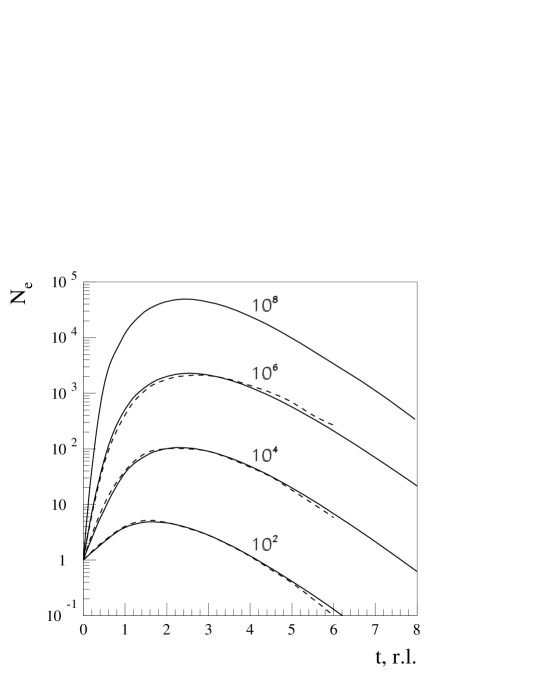
Figure 11: Cascade curves of electrons for showers initiated by primary electrons in the magnetic field. Different values (indicated at the curves) of the ratio of primary and threshold energies are assumed for the fixed $\chi_{th}=\varepsilon_{th}H/H_{\rm cr}=10^{3}$. For comparison, the results obtained in Ref. [24] are also shown (dashed curves).

Fig. 11 illustrates dependence of cascade curves on the primary energy in a deep quantum regime with the threshold value of the parameter $\chi_{\rm th}=10^{3}$. It is seen that the location of the cascade curve maximum $t_{\rm m}$ ranges within $2\div 3$ radiation lengths. In geometrical units this implies that the position of the cascade curve maximum increases with energy proportional to $\varepsilon_{0}^{1/3}$. The maximum electron number, $N_{\rm m}$, grows with $\varepsilon_{0}$ as $\sim\varepsilon_{0}^{0.7}$. Thus, the cascade development in the magnetic field in the quantum regime is somewhat intermediate between the cascades in matter and the photon gas.

Figure 12: Cascade curves of electrons (upper panel) and photons (bottom panel) for showers initiated by primary electrons (solid curves) and photons (dashed curves) in the magnetic field. Different values of the threshold energy ($\varepsilon_{\rm th}$) are assumed for the fixed $\varepsilon_{0}=2\cdot 10^{7}$ and $H=10^{11}$ G. The $\varepsilon_{0}/\varepsilon_{\rm th}$ ratios are indicated at the curves. The corresponding values for $\chi_{\rm th}$ are presented in Table 5.

Table 5: The ratio $N_{\gamma}/N_{e}$ for cascade curves presented in Figure 12.

$\varepsilon_{0}/\varepsilon_{\rm th}$	$10^{2}$	$10^{4}$	$10^{5}$	$10^{6}$	$10^{8}$
$\chi_{\rm th}$	$4.5\cdot 10^{2}$	4.5	$4.5\cdot 10^{-1}$	$4.5\cdot 10^{-2}$	$4.5\cdot 10^{-4}$
$t=$0.3 r.l.	0.76	0.92	1.44	2.66	5.95
$t=$0.9 r.l.	0.94	1.09	2.73	4.65	1.92
$t=$3 r.l.	1.00	1.17	11.2	18.6	45.2
$t=$6 r.l.	1.03	1.19	107	140	455

In Fig. 12 we present the cascade curves of electrons and photons for different values of the threshold energy $\varepsilon_{\rm th}$. It is seen that in the regime $\chi_{\rm th}\ll 1$ the cascade curves have a behaviour quite similar to that for the cascade curves in the photon gas shown in Figure 10. This can be explained by similarities of the synchrotron radiation and the Compton scattering in the non-quantum regime. In both cases the electrons suffer a large number of collisions but with small energy transfer to secondary photons. In addition, in both cases $\gamma$-rays stop to interact effectively with the ambient medium.

Table 5 demonstrates the dependence of the $N_{\gamma}/N_{\rm e}$ ratio on $\chi_{\rm th}$ and $t$. It behaves quite similar to cascades in matter. Particularly, for large threshold energies $\varepsilon_{\rm th}$ the electron and photon numbers are comparable; for small $\varepsilon_{\rm th}$ the photon number is considerably larger, and the ratio $N_{\gamma}/N_{\rm e}$ increases with the depth.

4.2 Energy spectra of cascade particles

Compared to the cascade curves, the energy spectra of electrons and photons at different stages of the cascade propagation contain more circumstantial information about the shower characteristics.

Figure 13: Differential energy spectra of electrons (solid curves) and photons (dashed curve) for cascades initiated in the hydrogen gas by a primary photon with energy $\varepsilon_{0}=2\cdot 10^{8}$. Different values of depths in units of the cascade maximum $t_{\rm m}$ are shown at the curves.

In Fig. 13 we show the energy spectra of cascade electrons and photons at different penetration depths in the hydrogen gas. At energies exceeding the critical energy, $\varepsilon\gg\varepsilon_{\rm cr}$, the spectra of both electrons and photons are described by power-law $dN/d\varepsilon\sim\varepsilon^{-\alpha}$, where the spectral index is function of the penetration depth. Near the shower maximum, $\alpha\simeq$2 for both electron and photon spectra. With depth the spectra become steeper.

Figure 14: Differential energy spectra of cascade electrons (upper panel) and photons (bottom panel) in the cascade initiated by a primary photon ($\kappa_{0}=10^{3}$) in the radiation field with Planckian spectral distribution. The spectra are calculated for different penetration depths indicated (in units of radiation lengths) at the curves.

Below the critical energy, the cross-sections of the bremsstrahlung and pair-production processes are not sufficiently large to support the cascade development against the dissipative processes like ionization and Compton scattering. Thus the multiplication of cascade particles is dramatically reduced. The cooling time of electrons due to ionization losses is proportional to energy, therefore below the critical energy this process leads to significant hardening of the electron, and correspondingly also the photon spectrum that behaves as ${\rm d}N/{\rm d}\varepsilon\propto\varepsilon^{-1}$.

In Fig. 14 we show the differential energy spectra of cascade particles in the radiation field with Planckian type spectral distribution. These spectra are quite different from the ones that appear in the cascades developed in matter. In the high energy (Klein-Nishina) region, $\kappa=\varepsilon\omega_{0}\gg 1$, and for not very large depths ($t\leq 10$ r.l.) the shape of the differential spectra of electrons and photons is quite insensitive to the depth (contrary to the cascade in matter). At these energies the differential spectra are characterized by slopes with indices between 1 and 1.5.

At $\kappa\sim 1$ there exists a pronounced transition region where the energy spectra undergo dramatic changes. The reason for the appearance of the transition region is the change of the character of Compton scattering (from the Thompson to the Klein-Nishina regime) and the sharp reduction of the pair production cross-section. Obviously, a broader energy distribution of background photons would make this transition smoother and less pronounced.

Figure 15: Differential energy spectra of cascade electrons (upper panel) and photons (bottom panel) in showers initiated in the magnetic field of intensity $H=10^{11}$ G by a primary photon of energy $\varepsilon_{0}=2\cdot 10^{7}$. The spectra are calculated at different depths indicated (in units of radiation lengths) at the curves.

At low energies ($\kappa\sim 1$) the cascade development is not supported by pair-production. Here we deal with an ensemble of photons not interacting with the environment and an ensemble of electrons continuously cooling down with the characteristic (Thompson) time $t_{\rm T}\sim 1/\varepsilon$. This results in standard electron spectra with spectral index $\alpha=2$. During propagating into deeper layers of the photon gas, these electrons produce large number of low energy photons with energy spectrum ${\rm d}N_{\gamma}/{\rm d}\varepsilon\propto\varepsilon^{-1.5}$.

For any finite depth $t$, electrons do not have enough time to be cooled down to energies $\varepsilon\to 0$. Therefore the electron spectrum drops dramatically below some energy $\tilde{\varepsilon}_{\rm e}$ which decreases with depth as $\sim 1/t$. This effect is clearly seen Fig. 14. The corresponding response in the photon spectrum is also quite distinct. Below the break energy around $\sim\omega_{0}\tilde{\varepsilon}_{\rm e}^{2}$, the photon spectrum becomes extremely hard, ${\rm d}N_{\gamma}/{\rm d}\varepsilon\approx const$.

The energy spectra of electrons and photons produced during the cascade development in the magnetic field are quite similar to the spectra of electromagnetic cascades in the radiation field with Planckian distribution of target photons. These spectra are shown in Fig. 15. All features discussed above in the context of cascading in the photon gas, are clearly seen also in cascades developed in the magnetic field, if we express the penetration depths in units of radiation lengths, and the energies of electrons and photons in the form of products $\varepsilon\omega_{0}$ and $\varepsilon(H/H_{\rm cr})$. The cascade spectra in radiation and magnetic fields are not, however, identical. For example, because of significant differences in the asymptotics of relevant cross-sections, $\gamma$-ray  spectra in the magnetic field in the quantum regime are flatter than the corresponding $\gamma$-ray  spectra in the photon gas in the Klein-Nishina regime (compare Figs. 14 and 15).

5 Mixed environment

In order to reveal peculiarities of the cascade development in different substances, in previous sections we limited our discussion to the “clean” environments dominated by matter, radiation or magnetic fields. The “pure cascade” concept is not only a convenient theoretical approximation. In fact, under certain realistic conditions and within limited energy regions, this could be the most likely realization of particle interactions with then ambient medium. The relativistic electron-photon cascades in the Earth’s atmosphere, in the intergalactic medium and in pulsar magnetospheres are 3 characteristic examples of “pure” cascade developments in matter, photon gas and magnetic field, respectively.

In some cases, however, “parallel” interactions of electrons and photons with 2 or 3 substances can proceed simultaneously and with comparable efficiencies. The outcome of the interference of several competing processes could be quite different and complex depending on relative densities of the ambient plasma, radiation and magnetic fields, as well as on the energy of primary particles. For example, interactions of $\geq 10^{20}\ \rm eV$ protons with 2.7 K CMBR leads to production of secondary electrons, positrons and $\gamma$-rays of energy $\geq 10^{19}\ \rm eV$, which in their turn trigger electromagnetic cascades in the same radiation field. However, due to the synchrotron cooling of electrons this process would be significantly suppressed if the intergalactic magnetic field exceeds $10^{-10}\ \rm G$. The characteristic energy of synchrotron photons $\sim 5\times 10^{8}(B/10^{-10}\ \rm G)(E/10^{19}\ \rm eV)^{2}\ \rm eV$ is too small for interactions with the diffuse photon fields on the Hubble scales. However, if the energy of electrons and/or photons injected into the intergalactic medium exceeds $\geq 10^{21}\ \rm eV$ (this could be the case, for example, of secondary products from decays of the so-called topological defects), then the synchrotron photons appear in the TeV energy range. The TeV $\gamma$-rays  effectively interact with the diffuse extragalactic infrared radiation, and trigger new, low energy electron-photon cascades. In both cases the synchrotron radiation changes the character of the cascade development in the radiation field, but cannot support its “own” cascade in the magnetic field.

Below we briefly discuss a more interesting scenario, when the cascade develops both in the radiation and magnetic fields. Let’s assume that a $\gamma$-ray photon of energy $E_{\gamma}=10^{20}$ eV is injected into a highly magnetized low-density plasma with thermal radiation density comparable to the energy density of the magnetic field $H^{2}/8\pi$. In principle such a situation can occur in the vicinity of central engines of AGN.

Figure 16: The cascade curves of electrons (upper panel) and photons (bottom panel) with energy $E\geq E_{\rm th}=5\cdot 10^{11}$ eV for showers initiated by a primary photon of energy $E_{0}=10^{20}$ eV in a mixed environment consisting of the magnetic field and the blackbody radiation. The calculations are performed for 5 combinations of parameters characterizing the target radiation and magnetic fields. These parameters are listed in Table 6.

Table 6: Parameters of the mixed environment used for calculations of the cascade curves shown in Fig. 16. $H$ is the strength of the magnetic field, $T$ is the temperature of the black-body radiation, $w_{\rm F}$ and $w_{\rm G}$ are energy densities of the magnetic field and black-body radiation, respectively.

Parameter Combination	1	2	3	4	5
$H$, Gauss	100	0	100	100	10
$kT$, eV	–	3	0.3	3	0.3
$w_{F}$, erg/cm3	400	0	400	400	4
$w_{G}$, erg/cm3	0	$\simeq 10^{4}$	$\simeq 1$	$\simeq 10^{4}$	$\simeq 1$

Fig. 16 illustrates the impact of the magnetic field and the temperature of blackbody radiation on cascade curves. Five different combinations of these parameters presented in Table 6 have been analyzed. The minimum particle energy for the cascade curves was taken $5\times 10^{11}$ eV, i.e. comparable or larger (for the assumed radiation temperatures) to the effective pair production threshold in the black-body radiation , $E_{\rm th}^{\rm(G)}\sim m_{\rm e}^{2}c^{4}/kT\simeq 10^{11}(kT/1\ \rm eV)^{-1}\ \rm eV$.

For the chosen parameters, the radiation length in the magnetic field is much smaller than the mean free path of primary $\gamma$-rays in the photon field. At absence of magnetic field (parameter combination 2) primary $\gamma$-rays  penetrates very deep into the source without interacting with the ambient photon gas. Consequently, the cascade starts very late and remains as underdeveloped.

The presence of a strong magnetic field makes the cascade development much more effective, which now is supported by magnetic pair production and synchrotron radiation. The cascade develops in this regime until the energy of $\gamma$-rays is reduced down to the effective threshold of the magnetic pair production, $E_{\rm th}^{\rm(F)}\simeq 10^{17}(H/100\ \rm G)^{-1}\ \rm eV$. Therefore, in the case of pure magnetic field we have quite simple and predictable cascade curves (parameter combination 1).

The presence of photon gas changes significantly the character of cascade development. At energies above $E_{\rm th}^{(F)}$ both electrons and $\gamma$-rays  interact mainly with magnetic field. When the cascade particles enter the energy interval determined by the pair-production thresholds in the radiation and magnetic fields, [$E_{\rm th}^{(G)}$, $E_{\rm th}^{(F)}$], the $\gamma$-rays  interact effectively with the photon gas, while the electrons continue to interact mainly with the magnetic field. Although for $kT=3\ \rm eV$, the blackbody radiation density considerably exceeds the energy density of 100 G magnetic field (see Table 6), because of the Klein-Nishina effect the interactions of electrons with photon gas become significant only when the electrons are cooled down to energies $\leq 100$ GeV. The mean free path of $\gamma$-rays  in the black-body radiation field has minimum around $E_{\rm th}^{\rm(G)}$. Therefore, $\gamma$-rays  start to interact intensively with the ambient photons at depths comparable with the mean free path $\Lambda_{\rm min}\sim\Lambda_{\gamma}(E_{\rm th}^{\rm(G)})$. This results in a rapid growth of the electron cascade curve and reduction of the high energy photon cascade curve (parameter combinations 3-5). Due to the rapid synchrotron cooling, the mean free paths of very energetic electrons in the magnetic field are very short, therefore for each given depth the main source of these electrons are $\gamma$-rays  which can penetrate much deeper. On the other hand, due to the same synchrotron losses, the electrons cannot support reproduction of very high energy $\gamma$-rays. Therefore, the at depths $\gg\Lambda_{\rm min}$ both the electron and photon curves are suppressed.

The increase of the temperature increases the energy density of the photon gas ($\propto T^{4}$) and makes interactions of cascade particles with radiation more intensive. This results in faster absorption of cascade particles (parameter combination 4). The reduction of the magnetic field (parameter combination 5) leads to the increase of the magnetic radiation length, as well as to the increase of the magnetic pair production threshold. As a result, the cascade develops slower.

Figure 17 illustrates the spectral evolution of cascade $\gamma$-rays  calculated for $H=100\ \rm G$ and two different temperatures of the black-body radiation, $kT=0.3$ and 3 eV (parameter combinations 3 and 4). It is seen that at small depths ($t\leq 10^{10}$ cm for the upper panel and $t\leq 10^{8}$ cm for the bottom panel) the spectra are fully determined by interactions with the magnetic field. At these depths a “standard” power-law spectrum with $\alpha=1.5$ is formed in a broad energy region below $E_{\rm th}^{(F)}$. At larger depths the interactions with the photon gas start to deform the shape of the spectrum. These interactions lead to absorption of photons above $E_{\rm th}^{\rm(G)}$. At the same time, synchrotron radiation of the photo-produced pairs appears in the energy region $E\leq E_{\rm th}^{\rm(G)}$. Thus, only the photons with energy below $E_{\rm th}^{\rm(G)}$ can survive at large depths. The spectrum of these photons is close to power-law with photon index 1.8-1.9, i.e. steeper than the the canonical $\varepsilon^{-1.5}$ cascade photon spectrum formed in the pure photon gas or pure magnetic field. This is explained by the break of symmetry between electrons and $\gamma$-rays. While at late stages of the cascade development $\gamma$-rays  continue to produce high energy electron-positron pairs, the synchrotron cooling of these electrons does not anymore support the cascade, but rather destroys it.

Finally, in Fig. 18 we show the spectral evolution of cascade $\gamma$-rays  calculated for a less extreme combination of model parameters. Namely, compared to Fig. 17, we assume a smaller energy for primary $\gamma$-rays  ($E=10^{17}$ eV) and weaker magnetic field ($H=1$ G). At these conditions the primary photons do not interact with the magnetic field. Instead, the cascade development starts with pair production in the radiation field. Nevertheless, we can see that many basic features, in particular the $\varepsilon^{-2}$ type spectrum at low energies, are quite similar to the spectra shown in Fig. 17.

Figure 17: Differential energy spectra of $\gamma$-rays  of the cascade initiated by a primary photon of energy $E_{0}=10^{20}$ eV in the compound environment consisting of a blackbody radiation of temperature $T$ and a homogeneous magnetic field H=100 G. Upper panel – $kT=0.3~{}eV$; bottom panel – $kT=3$ eV. The spectra are calculated at different depths (in cm) indicated at the curves.

Figure 18: The same as in Fig. 17, but for the energy of primary photons $E_{0}=10^{17}$ eV and the magnetic field $H=1\ \rm G$. The temperature of the black-body radiation is assumed 0.3 eV.

6 Summary

In this study, the technique of adjoint cascade equations has been applied to investigate properties of electron-photon cascades in hydrogen gas and in ambient radiation and magnetic fields. We also have inspected the main features of cross-sections of relevant processes that initiate and support cascade developments in these substances.

The cascade curves of electrons and photons in the photon gas and magnetic field have features quite different from the cascade curves in matter. The energy spectra of cascade particles are also considerably different from the conventional cascade spectra in matter. The spectra for the magnetic field have properties intermediate between those for cascade spectra in matter and in the photon field. Although for certain astrophysical scenarios the development of cascades in “pure” environments can be considered as an appropriate and fair approximation, at some conditions the interference of processes associated with interactions of cascade electrons and $\gamma$-rays  with the ambient photon gas and magnetic field (or matter) can significantly change the character of cascade development, and consequently the spectra of observed $\gamma$-rays. The impact is very complex and quite sensitive to the choice of specific parameters. Therefore each practical case should be subject to independent studies.

References

- [1] B. Rossi, K. Greisen, Rev. Mod. Phys. 13 (1941) 419; J.Nishimura, Handbuch der Physik Bd.XLVI/2 (1967) 1; I.P Ivavenko, Electromagnetic Cascade Processes (1968), Moscow State University Press (in Russian); T.K. Gaisser, Cosmic Rays and Particle Physics (1990), Cambridge University Press.
- [2] W.R. Nelson, H. Hirayama, D. Rogers, Preprint SLAC-265 (1985), Standford University.
- [3] V.S. Berezinsky, S.V. Bulanov, V.A. Dogiel, V.L. Ginzburg, V.S. Ptuskin Astrophysics of cosmic rays (1991), Amsterdam: North-Holland.
- [4] V.S. Berezinsky, in Roberts A. (editor), Proc. 1976 DUMAND Summer Workshop (1976), FNAL, Batavia, p. 229; D. Eichler, W.T. Westrand, Nature 307 (1984) 613.
- [5] F. Halzen, D. Hooper, Rep. Prog. Phys. 65 (2002) 102.
- [6] F.A. Aharonian, V.V. Vardanian, V.G. Kirillov-Ugryumov, Astrophysics (tr. Astrofizika) 20 (1984) 118; F.A. Aharonian, V.V. Vardanian, Astr. Sp. Sci. 115 (1985) 31.
- [7] A.A. Zdziarski, Astrophys. J. 335 (1988) 786.
- [8] R. Svensson, MNRAS 227 (1987) 403.
- [9] P.S. Coppi, R.D. Blandford, MNRAS 245 (1990) 453.
- [10] A. Mastichiadis, R.J Protheroe, A.P. Szabo, MNRAS 266 (1994) 910.
- [11] G. Cavallo, M.J. Rees, MNRAS 183 (1978) 359; E.V. Derishev, V.V. Kocharovsky, Vl.V. Kocharovsky, Astron. Astrophys. 372 (2001) 107; C.D. Dermer, Astrophys. J. 574 (2002) 65.
- [12] K. Mannheim, Phys. Rev. D 48 (1993) 2408; R.D. Blandford, A. Levinson, Astrophys. J. 441 (1995), 79; A. Atoyan, C.D. Dermer, Phys. Rev. Lett. 87 (2001) 221102; A. Muecke, R.J. Protheroe, R. Engel, J.P. Rachen, T. Stanev, Astropart. Phys. (2002), in press;
- [13] P.L. Biermann, P.A. Strittmatter, Astrophys. J. 322 (1987) 643; K. Mannheim, P.L. Biermann, W.M. Kruells, Astron. Astrophys. 251 (1991) 723.
- [14] A. Neronov, D . Semikoz, F. Aharonian, O. Kalashev, Phys. Rev. Lett. 89 (2001) 1101.
- [15] F. A. Aharonian, MNRAS 332 (2002) 215.
- [16] F.A. Aharonian, P.S. Coppi, H.J. Völk, Astrophys. J. 423 (1994) L5.
- [17] F.A. Aharonian, A.M. Atoyan, Sov. Phys. JETP 62 (1985) 189; R.J. Protheroe, MNRAS 221 (1986) 769; F.A. Aharonian, B.L. Kanevsky, V.V. Vardanian, Astr. Sp. Sci 167 (1990) 93; I.P. Ivanenko, A.A. Lagutin, Proc 22nd ICRC (Dublin), 1991, vol. 1, p. 121; F.A. Aharonian, P. Bhattacharjee, D.N. Schramm, Physical Review D 46 (1992) 4188; R.J. Protheroe, T. Stanev, MNRAS (264) 191, 1993; R.J. Protheroe, T. Stanev, V.S. Berezinsky, Nucl. Phys. B 43 (1995) 62; R.J. Protheroe, T. Stanev, Phys. Rev. Letters 77 (1996) 3708; P.S. Coppi, F.A. Aharonian, Astrophys. J. 423 (1997) L9; G. Sigl, S. Lee, D. Schramm, P. Coppi, Phys. Letters B 392 (1997) 129; S. Lee, Phys. Rev. D 58 (1998) 043004, Z. Fodor, S.D. Katz, Phys. Rev. D 63 (2001) 023002; F.A. Aharonian, A.N. Timokhin, A.V. Plyasheshnikov, Astronon. Astrophys. 384 (2002) 834; O. Kalashev, V. Kuzmin, D. Semikoz, G. Sigl, Phys. Rev. D 65 (2002) 103003.
- [18] S. Bonometto and M. J. Rees, MNRAS 152 (1971) 21.
- [19] P.W. Guilbert, A. C. Fabian, M.J. Rees, MNRAS 205 (1983) 593.
- [20] F.A. Aharonian, V.G. Kririllov-Ugriumov, V. V. Vardanian, Astr. Sp. Sci. 115 (1985) 201.
- [21] P.A. Sturrock, Astrophys. J. 164 (1971) 529.
- [22] M.G. Baring, A.K. Harding, Astrophys. J. 547 (2001) 529.
- [23] B.L. Kanevsky and A.I. Goncharov, Voprosy atomnoy nauki i techniki 4 (1999) p. 1 (in Russian).
- [24] V. Anguelov, H. Vankov, J. Phys. G: Nucl. Part Phys. 25 (1999) 1755.
- [25] A.V. Plyasheshnikov, F.A. Aharonian, . J. Phys. G: Nucl. Part Phys. 28 (2002) 267.
- [26] W. Bednarek, MNRAS 285 (1997) 69.
- [27] A.I. Akhiezer, N.P. Merenkov, A.P. Rekalo J.Phys.G: Nucl. Part. Phys. 20 (1994) 1499.
- [28] L. D. Landau, G. Rumer, Proc. R. Soc A 166 (1938) 213.
- [29] V.V. Uchaikin, V.V. Ryzhov The Stochastic Theory of Transport of High Energy Particles (1998), Novosibirsk, Nauka (in Russian)
- [30] A.V. Plyasheshnikov, A.A. Lagutin, V.V. Uchaikin, Proc. of 16th ICRC (1979), Kyoto, vol. 7, p.1 .
- [31] R.W. Brown, W.F. Hunt, K.O. Mikaeilian, I.J. Muzinich, Phys. Rev. D 8 (1973) 3083.
- [32] A. Mastichiadis, MNRAS 253 (1991) 235; C.D. Dermer, R. Schlickeiser, Astron. Astrophys. 252 (1991) 414.
- [33] S.L. Adler, Ann. Phys. 67 (1971) 599.
- [34] A.I. Akhiezer, V.B. Berestetskii, Quantum Electrodynamics, 1965, Interscience, New York.
- [35] G.R. Blumenthal, R.G. Gould, Review Mod. Phys. 42 (1971) 237.
- [36] F.A. Aharonian, A.M. Atoyan, A.M. Nagapetyan, Astrophysics (tr. Astrofizika) 19 (1983) 187.
- [37] A.K. Konopelko, A.V. Plyasheshnikov, Nucl. Instr. Meth. 450 (2000) 419.