BeppoSAX Observations of Synchrotron X–ray Emission from Radio Quasars

Abstract

We present new BeppoSAX LECS, MECS, and PDS observations of four flat–spectrum radio quasars (FSRQ) having effective spectral indices $\alpha_{\rm ro}$ and $\alpha_{\rm ox}$ typical of high-energy peaked BL Lacs. Our sources have X–ray–to–radio flux ratios on average $\sim 70$ times larger than “classical” FSRQ and lie at the extreme end of the FSRQ X–ray–to–radio flux ratio distribution. The collected data cover the energy range $0.1-10$ keV (observer’s frame), reaching $\sim 100$ keV for one object. The BeppoSAX band in one of our sources, RGB J1629+4008, is dominated by synchrotron emission peaking at $\sim 2\times 10^{16}$ Hz, as also shown by its steep (energy index $\alpha_{\rm x}\sim 1.5$) spectrum. This makes this object the first known FSRQ whose X–ray emission is not due to inverse Compton radiation. Two other sources display a flat BeppoSAX spectrum ($\alpha_{\rm x}\sim 0.7$), with weak indications of steepening at low X–ray energies. The combination of BeppoSAX and ROSAT observations, (non-simultaneous) multifrequency data, and a synchrotron inverse Compton model suggest synchrotron peak frequencies $\approx 10^{15}$ Hz, although a better coverage of their spectral energy distributions is needed to provide firmer values. If confirmed, these values would be typical of “intermediate” BL Lacs for which the synchrotron and inverse Compton components overlap in the BeppoSAX band. Our sources, although firmly in the radio–loud regime, have powers more typical of high–energy peaked BL Lacs than of FSRQ, and indeed their radio powers put them near the low–luminosity end of the FSRQ luminosity function. We discuss this in terms of an anti-correlation between synchrotron peak frequency and total power, based on physical arguments, and also as possibly due to a selection effect.

1 Introduction

Blazars constitute one of the most extreme classes of active galactic nuclei (AGN), distinguished by their high luminosity, rapid variability, high ($>3$%) optical polarization, radio core–dominance, and apparent superluminal speeds (Kollgaard, 1994; Urry & Padovani, 1995). The broad–band emission in these objects, which extends from the radio to the gamma–ray band, appears to be dominated by non–thermal processes from the heart of the AGN, often undiluted by the thermal emission present in other AGN. Therefore, blazars represent the ideal class to study to further our understanding of non–thermal emission in AGN.

The blazar class includes BL Lacertae objects, characterized by an almost complete lack of emission lines, and a subclass of radio quasars (which by definition display broad emission lines) which have been variously called highly polarized quasars (HPQ), optically violently variable quasars (OVV), core-dominated quasars (CDQ). One of their observational properties which is easier to define is the flat–spectrum radio emission ($\alpha_{\rm r}\lesssim 0.5$) and so we will refer to them as flat–spectrum radio quasars (FSRQ).

Given the lack of prominent emission lines in BL Lacs, more than 95% of all known such objects have been discovered either in radio or X–ray surveys. Follow–up work on radio– and X–ray–selected samples has shown that the two selection methods yield objects with somewhat different properties. The energy output of most radio selected BL Lacs peaks in the IR/optical band (Giommi & Padovani, 1994; Padovani & Giommi, 1995, 1996); such objects are now referred to as LBL (low-energy peaked BL Lacs). By contrast, the energy output of most X–ray selected BL Lacs (referred to as HBL: high-energy peaked BL Lacs) peaks at UV/X–ray energies.

Padovani & Giommi (1995) and Sambruna, Maraschi & Urry (1996) have demonstrated that the difference in broad-band peaks for HBL and LBL is not simply phenomenological. Rather, it represents a fundamental difference between the two sub–classes. The location of the broadband peaks also suggests a different origin for the X–ray emission of the two classes. Namely, an extension of the synchrotron emission likely responsible for the lower energy continuum in HBL, which typically display steep (energy index $\alpha_{\rm x}\sim 1.5$) X–ray spectra, and inverse Compton emission in LBL, which have harder ($\alpha_{\rm x}\sim 1$) spectra (Perlman et al., 1996; Urry et al., 1996; Padovani & Giommi, 1996). BeppoSAX observations of BL Lacs are confirming this picture (Wolter et al., 1998; Padovani et al., 2001; Beckmann et al., 2002).

In this respect, one could expect to find a similar range in peak frequencies in the FSRQ class – for which, until recently, no evidence existed. Indeed, it was suggested by some authors (Sambruna, Maraschi & Urry, 1996), based upon the similarities of the optical–X–ray broad-band spectral characteristics of LBL and FSRQ, that no FSRQ with synchrotron peak emission in the UV/X–ray band should exist.

Two studies have drastically changed this picture: 1. the multifrequency catalog of Padovani, Giommi, & Fiore (1997) identified more than 50 FSRQ ($\sim 17$% of the FSRQ in their catalog) spilling into the region of parameter space once exclusively populated by HBL; 2. about 30% of FSRQ found in the deep X–ray radio blazar survey (DXRBS) (Perlman et al., 1998; Landt et al., 2001) were found to have X–ray–to–radio luminosity ratios, $L_{\rm x}/L_{\rm r}$, typical of HBL ($L_{\rm x}/L_{\rm r}\gtrsim 10^{-6}$ or $\alpha_{\rm rx}\lesssim 0.78$), but broad (FWHM $>2,000{\rm~{}km~{}s^{-1}}$) and luminous ($L>10^{43}{\rm~{}erg~{}s^{-1}}$) emission lines typical of FSRQ. The discovery of a large population of “X–ray strong” FSRQ (labeled HFSRQ by Perlman et al. (1998) to parallel the HBL moniker) represents a fundamental change in our perception of the broadband emission of FSRQ.

X–ray observations of these objects play a fundamental role in finding their place within the blazar class. For example, if the X–ray spectra were found to be relatively steep, one could infer a dominance of synchrotron emission, as observed in HBL. Flatter X–ray spectra, with corroborating evidence from the whole broad-band emission (Padovani & Giommi, 1996), would instead suggest inverse Compton emission. In the latter case, the simple equations ${\rm LFSRQ}\equiv{\rm LBL}$ (where by LFSRQ we mean the “typical” FSRQ with low-energy synchrotron peak) and ${\rm HFSRQ}\equiv{\rm HBL}$ would not be valid, and some more complicated explanation for the existence of this class should be sought.

Our previous knowledge of the X–ray spectra of this new class of objects is scanty and mostly based on low signal–to–noise ratio (S/N) ROSAT data (Padovani et al. 1997; Padovani et al., in preparation) and is therefore also limited to the relatively narrow $0.1-2.4$ keV band. The BeppoSAX satellite (Boella et al., 1997a), with its broad-band X–ray ($0.1-300$ keV) spectral capabilities, is particularly well suited for a detailed analysis of the individual X–ray spectra of these sources.

In this paper we present BeppoSAX observations of four HFSRQ candidates, selected as described below. In § 2 we present our sample, § 3 discusses the observations and the data analysis, while § 4 describes the results of our spectral fits to the BeppoSAX data. § 5 discusses the ROSAT data, § 6 presents the spectral energy distributions and synchrotron-inverse Compton fits to the data, § 7 discusses our results, while § 8 summarizes our conclusions. Throughout this paper spectral indices are written $S_{\nu}\propto\nu^{-\alpha}$ and the values $H_{0}=50$ km s^-1 Mpc^-1 and $q_{0}=0$ have been adopted.

Readers wanting to skip the details of the data reduction and go directly to our results can read § 2, the summaries of our BeppoSAX and ROSAT results in §§ 4.5 and 5.4, and then go straight to § 6.

2 The Sample

The sample selection was done in two separate steps, as our objects were observed in the BeppoSAX Cycle 2 and 3. For both cycles we defined as HFSRQ flat–spectrum quasars with $\alpha_{\rm ro}$, $\alpha_{\rm ox}$, and $\alpha_{\rm rx}$ values within $2\sigma$ from the mean values of the HBL in the multifrequency AGN catalog of Padovani, Giommi, & Fiore (1997). These are the usual effective spectral indices defined between the rest-frame frequencies of 5 GHz, 5,000 Å, and 1 keV. X–ray and optical fluxes have been corrected for Galactic absorption. The effective spectral indices have been K-corrected using the appropriate radio and X–ray spectral indices, available for most sources (otherwise mean values were assumed). Optical fluxes at 5,000 Å have been derived and K-corrected as described in Padovani et al. (in preparation). We have chosen this definition so that our selection of HFSRQ matches the traditional “HBL box” as detailed in, e.g., Padovani & Giommi (1995).

The $\alpha_{\rm ro}-\alpha_{\rm ox}$ plane for flat–spectrum radio quasars (FSRQ) and HBL BL Lacs. Triangles represent FSRQ, crosses represent HBL, while filled circles represent our sources. The region in the plane within $2\sigma$ from the mean $\alpha_{\rm ro}$, $\alpha_{\rm ox}$, and $\alpha_{\rm rx}$ values of HBL is indicated by the solid lines. Data from the multifrequency AGN catalogue of Padovani, Giommi, & Fiore (1997).

Table 1: Sample Properties.

Name	RA(J2000)	Dec(J2000)	$z$	O	E	F5GHz	$\alpha_{\rm r}$	$\alpha_{\rm ro}$	$\alpha_{\rm ox}$	$\alpha_{\rm rx}$	Galactic NH
						mJy				$10^{20}$ cm-2
WGA J0546.6$-$6415	05 46 41.8	$-$64 15 22	0.323	16.0	14.7	287	$-0.67$	0.39	1.17	0.66	4.54
RGB J1629$+$4008	16 29 01.3	$+$40 08 00	0.272	17.6	17.1	20	$-0.29$	0.34	0.93	0.54	0.85
RGB J1722$+$2436	17 22 41.2	$+$24 36 19	0.175	16.5	15.1	35	$-0.75$	0.26	1.34	0.63	4.95
S5 2116+81	21 14 01.2	$+$82 04 48	0.084	14.6	13.3	376	$0.26$	0.31	1.41	0.69	7.41

Table 2: BeppoSAX Journal of observations.

Name	LECS	LECS	MECS	MECS	PDS	PDS	Observing Date
	exp. (s)	count rate (cts/s)	exp. (s)	count rate (cts/s)	exp. (s)	count rate (cts/s)
WGA J0546.6$-$6415	18564	$0.036\pm 0.002$	47234	$0.053\pm 0.001$	20004	$0.148\pm 0.059$	1998 Oct 1-2
RGB J1629$+$4008	20512	$0.033\pm 0.002$	44759	$0.023\pm 0.001$	22798	$0.086\pm 0.054$	1999 Aug 11-12
RGB J1722$+$2436	12175	$0.008\pm 0.003$	43993	$0.053\pm 0.001$	19732	…	2000 Feb 13-14
S5 2116$+$81	13171	$0.147\pm 0.004$	28826	$0.218\pm 0.003$	13296	$0.286\pm 0.073$	1998 Apr 29
S5 2116$+$81	05575	$0.107\pm 0.006$	19674	$0.162\pm 0.003$	10488	$0.240\pm 0.084$	1998 Oct 12-13

In January 1998, for Cycle 2, we selected the four X–ray brightest HFSRQ candidates then known. Three of these came from the AGN catalog of Padovani, Giommi, & Fiore (1997), while the fourth one was the X–ray brightest HFSRQ in the DXRBS list of Perlman et al. (1998). We were granted BeppoSAX observing time for two of these sources. In January 1999, for Cycle 3, we were able to select even more extreme candidates by using the ROSAT-Green Bank survey (RGB) (Brinkmann et al., 1997; Laurent-Muehleisen et al., 1998). Being based on the ROSAT All-Sky Survey (RASS) the RGB sample has an X–ray flux limit higher than DXRBS ($f_{\rm x}\sim 2\times 10^{-13}$ erg cm^-2 s^-1 vs. $\sim{\rm a~{}few}\times 10^{-14}$ erg cm^-2 s^-1) while it reaches slightly lower 5 GHz radio fluxes ($f_{\rm r}\sim 25$ mJy vs. $\sim 50$ mJy). RGB sources have then, by selection, higher $f_{\rm x}/f_{\rm r}$ ratios, that is lower $\alpha_{\rm rx}$, as needed to get more extreme (with synchrotron peaks, $\nu_{\rm peak}$, at higher energies) HFSRQ. The identification of FSRQ from the RGB sample is based on a cross-correlation with the NRAO VLA (Very Large Array) Sky Survey (NVSS) (Condon et al., 1998) at 1.4 GHz and is described in detail in Padovani et al. (in preparation). Amongst all FSRQ in the HBL region with $\alpha_{\rm rx}<0.65$ which, based on HBL spectral energy distributions (SEDs), would correspond to $\nu_{\rm peak}\gtrsim 10^{16}$ Hz (Fossati et al., 1998), we again selected the four X–ray brightest HFSRQ candidates and, again, were granted BeppoSAX observing time for two out of four sources.

The object list and basic characteristics are given in Table 1, which presents the source name, position, redshift, $O$ (blue) and $E$ (red) magnitudes from the Automatic Plate Measuring (APM) (Irwin et al., 1994), 5 GHz radio flux, radio spectral index, $\alpha_{\rm ro}$, $\alpha_{\rm ox}$, and $\alpha_{\rm rx}$ values, and Galactic N_H.

Figure 1 shows the $\alpha_{\rm ro}-\alpha_{\rm ox}$ plane for FSRQ and HBL and the location of our sources, well within the region which includes $\sim 95$% of HBL and clearly offset from where most FSRQ are located. Note that, in fact, our objects have $\langle\alpha_{\rm rx}\rangle=0.63\pm 0.03$. For comparison, the FSRQ with X–ray data belonging to the 2 Jy sample ($\sim 80$% of the total), which include all “classical” FSRQ (e.g., 3C 273, 3C 279, 3C 345, 3C 454.3: Padovani (1992)), have $\langle\alpha_{\rm rx}\rangle=0.87\pm 0.01$, which corresponds to an X–ray–to–radio flux ratio $\sim 70$ times smaller. We anticipate that our sources have powers which, although within the FSRQ range, are relatively low, as discussed in §§  7.2.4 and 7.3.

The light curve of the two merged MECS units for RGB J1629$+$4008, along with its hardness ratio, defined as the ratio between the count rates in the 4–10 keV and 1.5–4 keV bands.

3 Observations and Data Analysis

Table 3: Single power–law fits, LECS + MECS.

Name	NH	$\alpha_{x}$	$F_{1keV}$	$F_{[2-10]}$	$F_{[0.1-2.4]}$	Norm	$\chi^{2}_{\nu}$/dof	F–test, notes
	$10^{20}$ cm-2		$\mu$Jy	erg cm-2 s-1	erg cm-2 s-1	(L/M)		fixed-free NH
WGA J0546.6$-$6415	4.54 fixed	$0.72\pm 0.08$	$0.64\pm 0.07$	3.84e-12	4.14e-12	0.82	1.07/41
	$4.60^{+3.59}_{-1.94}$	$0.72\pm 0.10$	$0.64\pm 0.08$	3.84e-12	4.15e-12	0.82	1.09/40	4%
RGB J1629+4008	0.85 fixed	$1.50\pm 0.06$	$0.66\pm 0.05$	1.25e-12	7.96e-12	0.67	0.90/28
	$0.58^{+0.50}_{-0.43}$	$1.45\pm 0.11$	$0.63\pm 0.06$	1.27e-12	7.19e-12	0.67	0.88/27	79%
RGB J1722+2436	4.95 fixed	$0.62\pm 0.22$	$0.16\pm 0.05$	1.07e-12	9.77e-13	0.81	0.63/18
	$1.02$ ($<14.6$)	$0.58^{+0.24}_{-0.23}$	$0.14\pm 0.05$	1.08e-12	8.85e-13	0.79	0.55/17	92%
S5 2116+81	7.41 fixed	$0.73\pm 0.04$	$2.71\pm 0.17$	1.61e-11	1.77e-11	0.77	0.96/61	1998 Apr 29
	$10.3^{+4.6}_{-3.0}$	$0.75\pm 0.07$	$2.83\pm 0.22$	1.60e-11	1.87e-11	0.78	0.91/60	96%
	7.41 fixed	$0.77\pm 0.07$	$2.15\pm 0.19$	1.19e-11	1.43e-11	0.67	0.98/46	1998 Oct 12-13
	$7.85^{+7.20}_{-3.30}$	$0.77\pm 0.09$	$2.16^{+0.22}_{-0.19}$	1.19e-11	1.44e-11	0.67	1.00/45	16%
	7.41 fixed	$0.74\pm 0.04$	$2.77\pm 0.16$	—	—	0.70	1.01/63	sum
	$9.6^{+3.7}_{-2.6}$	$0.76\pm 0.06$	$2.87\pm 0.20$	—	—	0.70	0.97/62	92%

Table 4: Broken power–law fits, LECS + MECS.

Name	NH	$\alpha_{S}$	$\alpha_{H}$	Ebreak	$F_{1keV}$	$F_{[2-10]}$	Norm	$\chi^{2}_{\nu}$/dof	F–test
	$10^{20}$ cm-2			keV	$\mu$Jy	erg cm-2s-1	(L/M)
WGA J0546.6$-$6415	$8.70$ ($<20$)	$1.1^{+1.3}_{-0.3}$	$0.6^{+0.2}_{-0.5}$	$2.4^{+3.6}_{-1.0}$	$0.9^{+0.2}_{-0.1}$	3.91e-12	0.75	0.99/38	88%, 94%
RGB J1629+4008	0.85 fixed	$1.5(unc.)$	$1.7(unc.)$	$3.8(unc.)$	$0.7(unc.)$	1.22e-12	0.67	0.94/26	32%
RGB J1722+2436	4.95 fixed	$1.88$($>0.02$)	$0.6^{+0.2}_{-0.2}$	$0.9$($<4.7$)	$0.1\pm 0.1$	1.08e-12	0.80	0.59/16	75%
S5 2116+81	7.41 fixed	$0.4^{+0.4}_{-0.6}$	$0.76^{+0.06}_{-0.06}$	$1.1^{+2.6}_{-0.3}$	$2.7\pm 0.3$	1.60e-11	0.77	0.92/59	92%, 4/29/98

A complete description of the BeppoSAX mission is given by Boella et al. (1997a). The relevant instruments for our observations are the coaligned Narrow Field Instruments (NFI), which include one Low Energy Concentrator Spectrometer (LECS) (Parmar et al., 1997) sensitive in the 0.1 – 10 keV band; three (two after May 1997) identical Medium Energy Concentrator Spectrometers (MECS) (Boella et al., 1997b), covering the 1.5 – 10 keV band; and the Phoswich Detector System (PDS) (Frontera et al., 1997), sensitive in the $15-300$ keV band, coaligned with the LECS and the MECS. A journal of the observations is given in Table 2.

The data analysis was based on the linearized, cleaned event files obtained from the BeppoSAX Science Data Center (SDC) on-line archive (Giommi & Fiore, 1997). The data from the two MECS instruments were merged in one single event file by the SDC, based on sky coordinates. The event file was then screened with a time filter given by SDC to exclude those intervals related to events without attitude solution (i.e., conversion from detector to sky coordinates; see Fiore et al. (1999)). This was done to avoid an artificial decrease in the flux. As recommended by the SDC, the channels $1-10$ and above 4 keV for the LECS and $0-36$ and $220-256$ for the MECS were excluded from the spectral analysis, due to residual calibration uncertainties.

The spectral analysis was performed using the matrices and blank-sky background files released in November 1998 by the SDC, with the blank-sky files extracted in the same coordinate frame as the source file, as described in Padovani et al. (2001). Because of the importance of the band below 1 keV to assess the presence of extra absorption or soft excess (indicative of a double power–law spectrum), we have also checked the LECS data for differences in the cosmic background between local and blank-sky field observations, comparing spectra extracted from the same areas on the detector (namely, two circular regions outside the $10^{\prime}$ radius central region, located at the opposite corners with respect to the two on-board radioactive calibration sources).

We looked for time variability in every observation, binning the data in intervals from 500 to 4000 s, with null results except for RGB J1629$+$4008. This source, in fact, clearly varied during the observation ($\chi^{2}$-test probability of constancy $<10^{-7}$, see Fig. 2), doubling its MECS flux in about $\sim 15$ hours, with a more rapid decay of a factor of $\sim 4$ in about 7 hours at the end of the observation. The same pattern is present in the single MECS units light curves, and the background showed no significant flux variations. In spite of the flux variation, no appreciable spectral changes seem to be present. The hardness ratio, defined as the ratio between the count rates in the 4–10 keV and 1.5–4 keV bands, is constant (with a $\chi^{2}$-test probability $\sim 35$%). We have also looked for possible differences extracting the spectra in the “high” and “low” states (defined as $>$ or $<$ 0.03 cts/s, respectively), finding no significant differences between the spectral indices. The LECS data also show evidence of variability, although less significant than the MECS one ($\chi^{2}$-test probability of constancy $\sim 5-10\%$, depending on the bin size). We stress that our only variable source is also the only one whose X–ray band is clearly dominated by synchrotron emission (see next section).

Figure 1: Best fit to the WGA J0546.6$-$6415 data: a single power–law with Galactic column density. On the right we also include the PDS data. The PDS flux is above the LECS+MECS extrapolation due to the likely contribution of several X–ray sources in the field of view. See text for details.

4 Spectral Analysis

The spectral analysis was performed with the XSPEC 10.0 package. Using the program GRPPHA in HEAsoft, the spectra were rebinned with more than 20 counts in every new bin, using the rebinning files provided by the SDC. Various checks using different rebinning strategies have shown that our results are independent of the adopted rebinning within the uncertainties. The LECS/MECS normalization factor was left free to vary in the range 0.65–1.0, as suggested by the SDC (Fiore et al., 1999).

We fitted the combined LECS and MECS data both with single and broken power–law models, with Galactic and free absorption. The absorbing column density was parameterized in terms of N_H, the HI column density, with heavier elements fixed at solar abundances and cross sections taken from Morrison & McCammon (1983). The Galactic value was derived from the nh program at HEASARC (based on Dickey & Lockman (1990)). The N_H parameter was set free to vary for all sources to check for internal absorption and/or indications of a “soft excess”. The main results of our single power–law fits are reported in Tab. 3. The $F$-test probability quantifies how significant is the decrease in $\chi^{2}$ due to the addition of a new parameter (free N_H). The errors quoted on the fit parameters are the 90% uncertainties for one and two interesting parameters, for Galactic and free N_H respectively. The errors on the 1 keV flux reflect the statistical errors only and not the model uncertainties. The results for the broken power–law fit to the data are presented in Tab. 4. $\alpha_{\rm S}$ and $\alpha_{\rm H}$ are the soft and hard energy indices respectively. In this case the $F$-test probability quantifies the decrease in $\chi^{2}$ due to the addition of two parameters (from a single power–law fit to a broken power–law fit). The errors quoted in this case are the 90% uncertainties for two interesting parameters.

We now discuss the details and results of the analysis for each objects.

4.1 WGA J0546.6$-$6415

This source is located near the Large Magellanic Cloud (LMC) at $\sim 51\arcmin$ from LMC–X3. Towards the edges of the LECS and MECS images (in the region at right ascension $<$ 05^h 46^m), apparently diffuse emission is visible, consistent with the emission of some sources in the LMC already catalogued through ROSAT PSPC observations (see Haberl & Pietsch (1999); hereafter HP99). The most intense source is at $\sim 11\arcmin$ from the quasar, with a count rate $\sim 20$% that of the quasar in the MECS images. It is spatially coincident with the source [HP99]0049, identified as a foreground star in HP99. Due to the presence of serendipitous sources we have used an extraction region of 4^′ also for the LECS instrument.

The data are well fitted by a single power–law model with Galactic absorption. The best fit plots and values are reported in Fig. 1 and Tab. 3. The obtained spectral index is flat ($\alpha_{\rm x}<1$), thus indicating an inverse Compton power–law origin of the emission, given the SED characteristics of this quasar (see § 6). This result at first glance does not seem to confirm the “HBL–like” nature of this object, suggested by its location in the $\alpha_{\rm ro}$ $-$$\alpha_{\rm ox}$ plane. We note, however, that a slightly better fit, even if not significantly improved, can be obtained with a broken power–law model, allowing for a column density higher than Galactic (N_H$\sim 8.7\times 10^{20}$ cm², $F$-test $\sim 88-94$%, where the two values refer to a comparison with a single power–law with free and Galactic N_H respectively; see Tab. 4). In this case, the steeper component below $\sim 2$ keV may indicate the presence of the tail of the synchrotron emission, as characteristic of “intermediate” BL Lacs (e.g., Giommi et al. 1999). Variability could also play a role in this (see § 5.1).

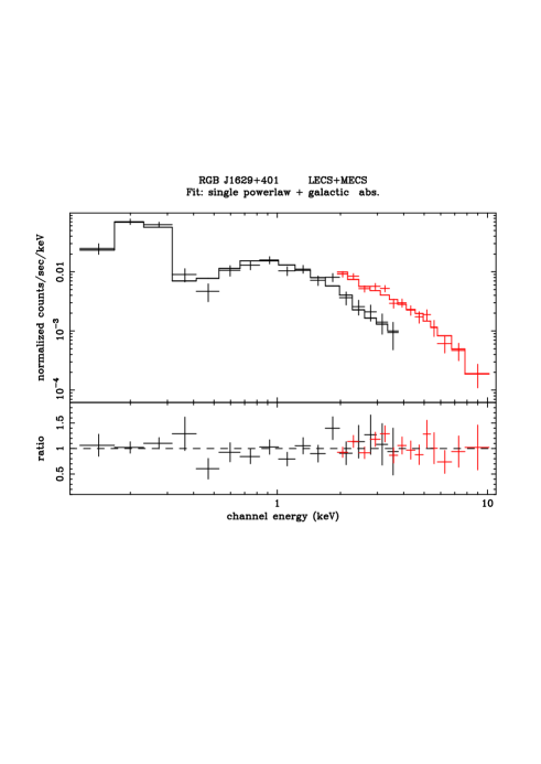
Figure 2: Single power–law fits to the LECS+MECS data of RGB J1629+4008, with absorption fixed at the Galactic value. On the right we include also the PDS data. The PDS flux is above the LECS+MECS extrapolation due to the contribution of A2199. See text for details.

Significant flux was detected also in the PDS instrument up to $\sim 60$ keV, but with a value not compatible with that expected by a simple extrapolation of the LECS+MECS spectrum (see Fig. 1, right). Due to the high number of X–ray sources in the field of view, we consider contamination the most likely explanation for this detection. In fact, there are 9 [HP99] sources within $40\arcmin$ from the quasar, with PKS 0552$-$640, an object classified as AGN in NED, at $40\arcmin$, and LMC-X3, a well known and bright X–ray binary source, at $\sim 51\arcmin$. Given the known X–ray spectrum of the latter (Haardt et al., 2001), we checked its possible contamination level using the published best fit model, after accounting for the off-axis efficiency of the instrument. Indeed, the hardest component, a power–law of index $\alpha_{\rm x}$ $\sim 1.7$ (Haardt et al., 2001), although steep, is quite strong ($\sim 10\mu Jy$ at 1 keV), and provides a non-negligible contribution up to $\sim 35-40$ keV.

4.2 RGB J1629+4008

This source is located 37^′ from the center of the well known cluster Abell (A) 2199. The X–ray emission from the hot gas of the cluster is clearly visible at the edges of the LECS and MECS images. To avoid contamination from the cluster, therefore, an extraction region of 6^′ has been used for the LECS. The best fit results are reported in Fig. 2 and Tab. 3. The spectrum is well fitted by a single power–law with Galactic values for the absorbing column density. The resulting spectral index is quite steep ($\alpha_{\rm x}$ $\sim 1.5$), as typical for HBL objects. This source therefore confirms its “HBL–like” properties also in the X–ray spectrum. We stress that RGB J1629+4008 is the first FSRQ ever found with synchrotron emission extending all the way to the X–ray band.

The PDS detected this source up to $\sim 35$ keV but the flux is more than an order of magnitude higher than expected from the LECS+MECS extrapolation (see Fig. 2, right). This is likely due to the cluster emission. A2199 is a very X–ray bright source (T $\approx 5$ keV, F${}_{[2-10]}=1.2\times 10^{-10}$ erg s^-1, emission integrated over a region of radius 20^′ ; De Grandi & Molendi (2002) and private communication) and, being at 37^′ from the quasar, is entirely within the PDS field of view and near where the PDS efficiency is still $\sim 50$% (42^′ ). Although its emission decreases exponentially towards higher energies, its high brightness still gives a flux in the 15–40 keV band $\sim 4.4\times 10^{-12}$ erg s^-1, higher than the quasar LECS+MECS extrapolation ($\sim 3.2\times 10^{-13}$ erg s^-1). As a check, we therefore fitted the LECS+MECS+PDS data including in the PDS the best fit model for the A2199 spectrum (De Grandi & Molendi, 2002), after accounting for the off-axis efficiency. In such a case the PDS data are well accounted for, with a total $\chi_{\nu}^{2}$$=1.03$ (as compared to 1.38 without the cluster contribution).

Note that for completeness we also fitted the data for this source with a broken power–law with absorption fixed at the Galactic value (see Tab. 4). No improvement with respect to the single power–law fit case was obtained.

RGB J1722+243 single power–law model with Galactic absorption.

4.3 RGB J1722+2436

Figure 3: BeppoSAX data and fitted spectra for our two observations of S5 2116+81. The data are fitted with a single power–law model with Galactic absorption.

This source is the weakest of the four observed in the soft X–ray range (see the LECS count rates in Tab. 2). To enhance the S/N, therefore, we used a 6^′ extraction region for the LECS, as suggested by the SDC (Fiore et al., 1999). The source is not detected by the PDS. The data are well fitted by a flat ($\alpha_{\rm x}<1$) single power–law model with Galactic absorption (see Fig. 4.2 and Tab. 3). The residuals, however, show the presence of some soft excess below 0.5$-$0.6 keV. This is confirmed by the free N_H fit, which gives values below the Galactic one. Due to the low S/N and the narrow band affected, the significance is only marginal ($F$-test $\sim 92$%, last column in Tab. 3). A fit with a broken power–law with the absorption fixed at the Galactic value yields a steep low-energy component with $\alpha_{\rm x}$ $\sim 1.9$, though unconstrained (see Tab. 4). The improvement with respect to the single power–law fit and Galactic absorption is however not significant ($\sim 75$%)

The flatness of the X–ray spectrum, as for WGA J0546.6+6415, does not confirm the “HBL–like” nature of this objects as suggested by the broad band indices. However, the possible steeper component at soft X–ray energies, if confirmed, may be attributed to the tail of the synchrotron emission, thus locating the observed X–ray band in the “valley” between synchrotron and Compton emissions (see, in fact, Fig. 4). In this case, the quasar could be the FSRQ counterpart of “intermediate” BL Lacs. Again, variability could have also played a significant role.

4.4 S5 2116+81

This object was observed by BeppoSAX twice, six months apart (see Tab. 2). In both observations the source was detected in the PDS up to $\sim 90$ keV. The source varied between the two observations ($\sim 20$%), with the highest state in the first observation. Both datasets are well fitted by a flat single power–law model (see Fig. 3 and Tab. 3), with very similar spectral indices (within the errors). The PDS data agree, within the errors, with the extrapolation of the LECS+MECS spectrum. Given the similarity of the spectral properties, we have also added the event files to obtain a higher S/N spectrum, whose fit is also reported in Tab. 3.

The free N_H value agrees with the Galactic one in the second dataset (within the large errors), while there is a marginal indication of possible excess absorption in the first and the summed datasets, according to the $F$-test ($96$% and $92$%, respectively). A broken power–law model with Galactic absorption provides an equivalent fit (giving roughly the same $\chi_{\nu}^{2}$ of the free N_H fit), with a flatter index ($\alpha_{\rm x}$ $\sim 0.4$) below 1.1 keV; however the significance of the improvement is slightly less ($F$-test $\sim 92$%; see Tab. 4), due to the higher number of parameters. The flat spectral indices in both observations (i.e., flux states) classify this source as a standard FSRQ.

4.5 Summary

To summarize our BeppoSAX spectral results, the fitted energy indices are flat, $\alpha_{\rm x}\lesssim 0.8$, for all but one source. The mean value is $\alpha_{\rm x}=0.90\pm 0.20$ and the weighted mean is $\alpha_{\rm x}=1.03\pm 0.04$. This latter value is heavily weighted towards RGB J1629+4008, the only object with a steep ($\alpha_{\rm x}\sim 1.5$) slope. Excluding this source we derive a mean value $\alpha_{\rm x}=0.70\pm 0.04$ and a weighted mean $\alpha_{\rm x}=0.75\pm 0.05$.

Three of our sources may have a spectrum which is more complex than a single power–law, as also illustrated by the residuals to the single power–law fits. A double power–law model fitted to their spectra indicates, within the rather large errors, a low-energy ($E\lesssim 1$ keV) excess for WGA J0546.6+6415 and RGB J1722+2436, with a flatter component emerging at higher energies. In fact, the spectra are concave with quite a large spectral change, with $\alpha_{\rm S}-\alpha_{\rm H}\sim 0.5-1.3$, and energy breaks around $E\sim 1-2$ keV. The hard X–ray spectral index is $\alpha_{\rm H}\sim 0.6$, while $\alpha_{\rm S}\sim 1.1-1.9$. Although the fit is improved by using a double power–law model, an $F$-test shows that the improvement is more suggestive than significant, with probabilities $\sim 75-94$%. We do include RGB J1722+2436 here, despite its relative low $F$-test probability, as we believe that a best fit $N_{\rm H}$ value a factor $\sim 5$ below the Galactic one is highly unlikely and strongly suggestive of a soft excess. We also note that by adding up the $\chi^{2}$ values in Tab. 4, an $F$-test shows that the improvement in the fit provided by a double power–law model for the two sources together is significant at the $\sim 93$% level. S5 2116+81, on the other hand, shows a hint of a flatter component at low energies ($E\lesssim 1$ keV), with $\alpha_{\rm S}-\alpha_{\rm H}\sim-0.4$.

Table 5: WGA J0546.6$-$6415. ROSAT Journal of observations.

Obs. ID	Instrument	Off axis	Exposure time	Net count rate	Observing date
		(arcmin)	(sec.)	(cts/s)
rp140008n00	PSPC-C	37.63	1334	$0.103\pm 0.012$	1990 Jul 9
rp140638n00	PSPC-C	37.63	1500	$0.101\pm 0.011$	1990 Jul 10
rp140009n00	PSPC-C	21.98	1543	$0.124\pm 0.011$	1990 Jul 9
rp140639n00	PSPC-C	21.98	1628	$0.140\pm 0.011$	1990 Jul 10
rp400078n00	PSPC-B	51.66	7490	$0.156\pm 0.005$	1993 Apr 10

Table 6: WGA J0546.6$-$6415. ROSAT single power–law fits.

Obs.	NH	$\alpha_{\rm x}$	$F_{1keV}$	$F_{[0.1-2.4]}$	$\chi^{2}_{\nu}$/dof
	$10^{20}$ cm-2		$\mu$Jy	erg cm-2 s-1
PSPC-B	4.54 fixed	$1.29\pm 0.10$	$0.88\pm 0.06$	8.69e-12	0.61/31
PSPC-C sum8	4.54 fixed	$0.8^{+0.2}_{-0.3}$	$0.45\pm 0.05$	3.06e-12	1.09/16
PSPC-C sum9	4.54 fixed	$0.8^{+0.2}_{-0.2}$	$0.48\pm 0.04$	3.34e-12	1.01/14
PSPC-C fit total	4.54 fixed	$0.83^{+0.14}_{-0.15}$	$0.47\pm 0.03$	3.22e-12	1.00/32

In short, one of our sources appear to show an “HBL–like” X-ray spectrum, while the other three are characterized by flat “LBL–like” spectra. One, or possibly two, of these sources, however, show hints of concave X-ray spectra typical of “intermediate” BL Lacs.

5 ROSAT PSPC Data

In order to study possible variations of the X-ray spectral properties (and synchrotron peak) in these objects and have a better understanding of the underlying emission processes, we have also looked for other X–ray observations available, in particular from the ROSAT archive, to take advantage of the higher resolution and collecting area at low energies. We found Position Sensitive Proportional Counter (PSPC) observations for two sources, namely WGA J0546.6$-$6415 and RGB J1629+4008. These objects are located near two famous and well observed X–ray sources, i.e., LMC–X3 and A2199 respectively, and thanks to the wide field of view of the ROSAT satellite we could find observations where our targets were present as serendipitous sources. The journals of the ROSAT observations are reported in Tab. 5 and Tab. 7. A third object, RGB J1722$+$2436, was detected in the RASS (Voges et al., 1999). We now present the results of the ROSAT analysis, along with a comparison with the BeppoSAX results.

5.1 WGA J0546.6$-$6415

Many PSPC observations of the Large Magellanic Cloud region are present in the ROSAT public archive, both for B and C detectors, but most have short exposures ($\lesssim 1000$ s) and/or with the quasar at high off-axis angles. We therefore decided to analyze the best ones, i.e., the longest observation (7490 s, PSPC-B, pointed on LMC-X3), and those with the lowest off-axis displacement (PSPC-C). Table 5 reports the basic information, namely the observation sequence ID code, the detector used, the off-axis position of our quasar in the field of view, the exposure time, the net count rate full band and date of observation. The PSPC-C observations took place in the same epoch (1990 July 9 and 10), with the satellite often changing position between the two pointings (thus the two off-axis positions in the same day). The many short observations have been then reduced and summed together in a single dataset by the ROSAT data center.

We fitted all the PSPC-C datasets independently, with a single power–law model plus Galactic absorption, obtaining good fits with similar values for the spectral indices and normalizations, within the errors. To increase the S/N, therefore, we summed the event files for the two observations with the same source detector coordinates (i.e., same off-axis angle). The fit results are reported in Tab. 6, where “sum8” refers to the summed event files ..008n00 and ..638n00, and “sum9” refers to the summed event files ..009n00 and ..639n00. Given the similarity of the values, we have also fitted the two datasets together (sum8 and sum9), using the same model parameters for both (including normalization). The resulting fit is good ($\chi_{\nu}^{2}$$=1.00$) thus confirming that both datasets have compatible spectral properties.

Table 7: RGB J1629+4008. ROSAT Journal of observations.

Obs. ID	Instrument	off axis	exposure time	net count rate	Observing date
		(arcmin)	(sec.)	(cts/s)
rp150083n00	PSPC-C	35.28	10553	$0.641\pm 0.008$	1990 Jul 18
rp800644n00	PSPC-B	35.28	40999	$0.676\pm 0.004$	1993 Jul 25
rp701507n00	PSPC-B	00.29	5175	$0.960\pm 0.014$	1993 Jul 30

Table 8: RGB J1629+4008. ROSAT single power–law fits.

Obs.	NH	$\alpha_{\rm x}$	$F_{1keV}$	$F_{[0.1-2.4]}$	$\chi^{2}_{\nu}$/dof
	$10^{20}$ cm-2		$\mu$Jy	erg cm-2 s-1
rp150083n00	0.85 fixed	$2.03\pm 0.05$	$0.33\pm 0.02$	8.15e-12	2.16/53
	$0.7\pm 0.2$	$1.95\pm 0.14$	$0.34\pm 0.03$	7.43e-12	2.17/52
rp800644n00	0.85 fixed	$2.23^{+0.02}_{-0.04}$	$0.29\pm 0.01$	9.68e-12	2.12/52
	$0.82\pm 0.01$	$2.21^{+0.08}_{-0.04}$	$0.30\pm 0.01$	9.39e-12	2.14/51
rp701507n00	0.85 fixed	$2.15^{+0.06}_{-0.05}$	$0.33\pm 0.03$	9.48e-12	1.37/43
	$0.4\pm 0.2$	$1.88^{+0.14}_{-0.14}$	$0.34\pm 0.03$	6.74e-12	0.95/42

All datasets analyzed are well fitted by single power–law models with Galactic column density. The free N_H fits provide values around the Galactic ones, and other absorbing models and/or a broken power–law model do not improve the fits. The results seem to indicate a variation of the spectral properties for this source: the 1993 PSPC-B spectrum is characterized by a steep “HBL–like” slope ($\sim 1.3$), contrary to what obtained by both the 1990 PSPC-C and 1998 BeppoSAX observations, which agree with each other reporting a flat and roughly equal spectral index ($\sim 0.8$ and $0.7$ respectively). The 1990 and 1998 flux levels are similar, too, with the BeppoSAX flux about 30% higher than the ROSAT one. Compared to these, instead, in 1993 the quasar was in a high state, with a 0.1–2.4 keV flux more than 2.5 times higher than the 1990 values. The X–ray spectrum of this object, therefore, seems to have a “steeper when brighter” behavior, which may indicate a shift towards higher energies of the synchrotron peak during high states, when synchrotron emission dominates over inverse Compton in the X–ray band (Padovani & Giommi, 1996; Giommi et al., 1999).

It must be noted, however, that these considerations are based on the 1993 PSPC-B observation, which may be affected by possible calibration problems. In fact, it has the highest off-axis angle (it is near the edge of the field of view), and these regions are usually not well studied and calibrated. In addition, also possible PSPC-B spectral miscalibrations, as reported in Iwasawa, Fabian, & Nandra (1999) and Mineo et al. (2000), must be taken into account, as these might steepen the ROSAT slopes by $\sim 0.2-0.3$ (Mineo et al., 2000).

5.2 RGB J1629+4008

As for the previous object, we looked in the ROSAT public archive for the best observations possible, i.e., the longest ones and/or those with the lower off-axis angle. We found two very long observations of the cluster A2199 taken in 1990 and 1993 with the PSPC-C and B instruments, respectively. These included our target in the field of view with an offset of $\sim 35\arcmin$. We found also a pointed observation, taken 5 days after the long exposure on A2199. The basic information for these datasets is reported in Tab. 7.

Table 9: RGB J1629+4008. Other fits to the ROSAT datasets.

Name	NH	$\alpha_{S}$	$\alpha_{H}$	Ebreak	$F_{1keV}$	$F_{[0.1-2.4]}$	$\chi^{2}_{\nu}$/dof	F–test
	$10^{20}$ cm-2			keV	$\mu$Jy	erg cm-2 s-1
rp150083n00	0.85 fixed	$2.3^{+0.2}_{-0.1}$	$1.0^{+0.4}_{-0.5}$	$0.7\pm 0.2$	$0.23\pm 0.05$	8.70e-12	1.47/51	$>99.9$%
rp800644n00	0.85 fixed	$2.33^{+0.09}_{-0.07}$	$1.4^{+0.4}_{-0.7}$	$0.8\pm 0.2$	$0.25\pm 0.02$	9.95e-12	1.43/50	$>99.9$%
rp701507n00	0.85 fixed	$2.7^{+3.8}_{-0.4}$	$1.9^{+0.2}_{-0.3}$	$0.3^{+0.2}_{-0.1}$	$0.13\pm 0.08$	1.08e-11	0.91/41	$>99.9$%
		NH warm	$\alpha_{x}$	Ewindow	$F_{1keV}$	$F_{[0.1-2.4]}$	$\chi^{2}_{\nu}$/dof	F-test
		$z=0.03$		keV	$\mu$Jy	erg cm-2 s-1
rp150083n00	0.85 fixed	$11\pm 4$	$1.75\pm 0.09$	$0.30^{+0.18}_{-0.02}$	$0.54\pm 0.06$	8.77e-12	1.17/51	$>99.9$%
rp800644n00	0.85 fixed	$6.5^{+3.3}_{-2.4}$	$2.07\pm 0.07$	$0.49^{+0.07}_{-0.27}$	$0.38\pm 0.03$	9.78e-12	1.27/50	$>99.9$%
rp701507n00	0.85 fixed	$1.6^{+3.5}_{-1.2}$	$2.2^{+0.2}_{-0.1}$	$0.25^{+0.03}_{-0.06}$	$0.36\pm 0.05$	1.10e-11	1.04/41	$\gtrsim$99.8%

At first we fitted all datasets with a single power–law model, both with Galactic and free absorption, but these did not provide an adequate fit (see $\chi_{\nu}^{2}$ in Tab. 8). The presence of a more complex spectral shape is also indicated by the free N_H  fit of the on-axis observation (rp701507n00), which provided a good $\chi_{\nu}^{2}$ only with absorption values below the Galactic ones.

We therefore tried alternative models, reported in Tab. 9. The fits were significantly improved both adopting a broken power–law model with Galactic absorption (top three rows in Tab. 9), and adding a warm absorption component, at the redshift of the A2199 cluster, to the single power–law model (bottom three rows in Tab. 9). This under the hypothesis that, at $\sim 35\arcmin$ from the center, there is still a not negligible amount of cluster gas, likely partially ionized. The model used for the warm absorber is ZWNDABS in XSPEC, an approximation to the warm absorber using the photoelectric cross-sections in Balucinska-Church & McCammon (1992).

The results are a bit puzzling and do not settle clearly the question of which model should be preferred. The F-test does not help here, given that the number of model parameters is the same. The off-axis observations seem to be better fitted by the warm absorber model, according to the $\chi^{2}$-test (15-20% against 2%, see the $\chi_{\nu}^{2}$ in Tab. 9), but this is not confirmed by the on-axis observation, which has the best $\chi_{\nu}^{2}$ for the broken power–law model. Moreover, the obtained values for the extra (warm) absorption are different (at the 90% level), a fact which would imply a variable absorption with timescales less than five days (the time interval between the last two observations, i.e., rp800644 and rp701507), quite unlikely. For this reason, and possible feature calibration problems for the off-axis observations (outside the PSPC central rib ring), we consider the broken power–law model a better representation of these data.

In both cases, however, the spectral properties of the continuum for this object confirm its “HBL–like” character showed in the BeppoSAX observations, displaying steep spectra in all three datasets. This result is confirmed also accounting for the possible ROSAT miscalibration (i.e., subtracting a maximum $\Delta\alpha\sim 0.2-0.3$). The broken power–law fits, which show a flattening of the spectrum towards higher energies, may indicate that the inverse Compton contribution is becoming not negligible, i.e., that the region where the synchrotron and Compton emissions cross was only slightly beyond the ROSAT band.

5.3 RGB J1722$+$2436

This source is included in the RASS. Yuan et al. (1998) give a $0.1-2.4$ keV flux $\sim 4.2\times 10^{-12}$ erg cm^-2 s^-1, i.e., a factor $\sim 4$ larger than the BeppoSAX value, with a spectral index derived from the hardness ratio $\alpha_{\rm x}=1.27^{+0.26}_{-0.28}$, assuming Galactic absorption. This is steeper than the BeppoSAX value and again suggests a “steeper when brighter” behavior.

5.4 Summary

To summarize our ROSAT spectral results, the fitted energy indices are relatively steep, $\alpha_{\rm x}\sim 1.4$, steeper than the BeppoSAX values by $\Delta\alpha\approx 0.5$. Possible ROSAT miscalibrations are supposed to account for a steepening of the order $\Delta\alpha\sim 0.2-0.3$, so we regard this difference as significant. In two cases the source was also brighter, suggesting a “steeper when brighter” behavior, indicative of a shift of the synchrotron peak towards higher energies during high states. Overall, this indicates a non-negligible synchrotron component in the X-ray band, which actually dominates for RGB J1629+4008.

6 Spectral Energy Distributions

To address the relevance of our BeppoSAX data in terms of emission processes we have assembled multifrequency data for all our sources. The main source of information was NED, and the data are not simultaneous with our BeppoSAX observations. We also looked for near–infrared observations in the Two Micron All Sky Survey (2MASS) Second Incremental Release (Cutri et al., 2000), finding data only for WGA J0546.6$-$6415.

6.1 Optical Variability

Given that our fits are mostly based on X-ray and optical data and that the latter are particularly important to determine $\nu_{\rm peak}$, we need to address the non-simultaneity of the optical and X-ray observations. The optical fluxes of FSRQ are in fact known to show significant variability, which could influence our results. We have then investigated the range of optical variability of our sources, with the following results.

• WGA J0546.6$-$6415. This is a newly identified source from the DXRBS (Perlman et al. 1998). Nevertheless, we did find variability information using SuperCOSMOS Sky Survey (Hambly et al., 2001) data, spanning the period 1975 – 1986. In particular, the UK Schmidt telescope (UKST) and European Southern Observatory (ESO) red observations, taken at the end of 1985/beginning of 1986 and separated by 50 days, agree within 0.01 magnitude, and give $R\sim 15.2$. This is 0.5 magnitudes fainter than the $F=14.7$ magnitude given in the USNO A2.0 catalogue, which refers to mid 1980. The Guide Star Catalogue-II (GSC-II), available at http://www-gsss.stsci.edu/, gives $J=15.9\pm 0.2$ and $F=15.3\pm 0.2$ for 1989, which indicates a brightening of $\sim 0.6$ magnitudes compared to the UKST blue value of 16.5 for 1975.

• RGB J1629$+$4008. This is a Faint Images of the Radio Sky at Twenty centimeters (FIRST) (Becker et al., 1995) quasar. Helfand et al. (2001) have studied the long-term optical variability of FIRST quasars. They found that in 1953 Palomar Observatory Sky Survey (POSS I) observations this object was $\sim 0.4$ magnitudes fainter in $B$ and $\sim 0.6$ magnitudes fainter in $R$ than in 1996 CCD observations. The GSC-II gives $J=18.0\pm 0.4$ and $F=17.5\pm 0.4$ for 1993. This is perfectly consistent with the CCD $B$ and $R$ values given by Helfand et al. (2001).

• RGB J1722$+$2436. This source was identified as a quasar by Bond et al. (1977) due to its optical variability. These authors quote a range of photographic magnitude for this source between 15.7 and 16.7, with long “still-stands” between brief periods of activity. The GSC-II gives $J=16.7\pm 0.4$ and $F=15.2\pm 0.4$ for 1996, in good agreement with the $O$ and $E$ APM values given in Tab. 1.

• S5 2116$+$81. The GSC-II gives $J=14.4\pm 0.4$ for 1993, consistent with the APM $O$ value given in Tab. 1.

In summary, within the available optical data, our sources display maximum variability amplitude $\sim 0.5-1$ magnitudes. We have then conservatively assigned to the optical fluxes an error of 0.2 dex, which corresponds to $\pm 0.5$ magnitudes (see Fig. 4).

6.2 Synchrotron Inverse Compton Model Fits

The SEDs for our sources are shown in Figure 4. The BeppoSAX data have been converted to $\nu f_{\rm\nu}$ units using the XSPEC unfolded spectra after correcting for absorption. ROSAT data are shown by a bow–tie that represents the spectral index range.

To derive the intrinsic physical parameters which could account for the observed data we have fitted the SED of our sources with a homogeneous, one–zone synchrotron inverse Compton model as developed in Ghisellini, Celotti, & Costamante (2002). This model is very similar to the one described in detail in Spada et al. (2001; it is the “one–zone” version of it), and is characterized by a finite injection timescale, of the order of the light crossing time of the emitting region (as occurs, for example, in the internal shocks scenario, where the dissipation takes place during the collision of two shells of fluid moving at different speeds). In this model, the main emission comes from a single zone and a single population of electrons, with the particle energy distribution determined at the time $t_{\rm inj}$, i.e., at the end of the injection, which is the time when the emitted luminosity is maximized. Details of the model can be found in Ghisellini, Celotti, & Costamante (2002), who have applied it successfully to both low–power BL Lacs and powerful FSRQ. Here we summarize its main characteristics.

The source is assumed cylindrical, of radius $R$ and width $\Delta R^{\prime}=R/\Gamma$ (in the comoving frame, where $\Gamma$ is the bulk Lorentz factor). The particle distribution $N(\gamma)$ is assumed to have the slope $n$ [$N(\gamma)\propto\gamma^{-n}$] above the random Lorentz factor $\gamma_{\rm c}$, for which the radiative cooling time equals the injection time. The latter is assumed to be equal to the light crossing time (i.e., $t_{\rm inj}\sim\Delta R/c$). The electron distribution is assumed to cut–off abruptly at $\gamma_{\rm max}>\gamma_{c}$. Below $\gamma_{c}$ there can be two cases, depending on the values of $\gamma_{c}$ and $\gamma_{\rm min}$:

i) If $\gamma_{c}>\gamma_{\rm min}$, we have $N(\gamma)\propto\gamma^{-(n-1)}$ between $\gamma_{\rm min}$ and $\gamma_{\rm c}$ and $N(\gamma)\propto\gamma^{-1}$ below $\gamma_{\rm min}$.

ii) Alternatively, if $\gamma_{c}<\gamma_{\rm min}$, then $N(\gamma)\propto\gamma^{-2}$ between $\gamma_{\rm c}$ and $\gamma_{\rm min}$ and $N(\gamma)\propto\gamma^{-1}$ below $\gamma_{\rm c}$.

According to these assumptions, the random Lorentz factor $\gamma_{\rm peak}$ of the electrons emitting most of the radiation (i.e., emitting at the peaks of the SEDs) is determined by the relative importance of radiative losses and can assume values in the range $\gamma_{\rm min}$ to $\gamma_{\rm max}$.

Our sources have broad lines and therefore the contribution of the disk to the SED could be relevant. Furthermore, photons produced in the broad line region could contribute to the seed photon distribution for the inverse Compton scattering. We accounted for this by assuming that a fraction $\sim$ 10% of the disk luminosity $L_{\rm disk}$ is reprocessed into line emission by the broad line region (BLR), $L_{\rm BLR}$, assumed to be located at $R_{\rm BLR}$. $L_{\rm BLR}$ was estimated following Celotti, Padovani, & Ghisellini (1997) from the fluxes of the strongest broad lines. These were available for all our sources from our own spectrum (WGA J0546.6–6415; Perlman et al. (1998)), from published spectra kindly made available to us by Sally Laurent–Muehleisen (RGB J1629$+$4008 and RGB J1722$+$2436) and from Stickel, Kühr, & Fried (1993) (S5 2116$+$81). $R_{\rm BLR}$ is assumed to scale as $L_{\rm disk}^{0.7}$, following Kaspi et al. (2000). Disk emission is assumed to be a simple black–body peaking at $10^{15}$ Hz. Within these assumptions, we can fix two important parameters for our modeling, and we can reliably estimate the importance of the seed photons produced externally to the jet for the Compton scattering process.

The source is assumed to emit an intrinsic luminosity $L^{\prime}$ and to be observed with the viewing angle $\theta$. The model parameters are listed in Table 10, which gives the name of the source in column (1), $L^{\prime}$ in column (2), $L_{\rm disk}$ in column (3), $R_{\rm BLR}$ in column (4), the magnetic field $B$ in column (5), the size of the region $R$ in column (6), the Lorentz factor $\Gamma$ in column (7), the viewing angle $\theta$ in column (8), the slope of the particle distribution $n$ in column (9), the minimum Lorentz factor of the injected electrons $\gamma_{\rm min}$ in column (10), and $\gamma_{\rm peak}$ and $\nu_{\rm peak}^{\rm syn}$ in columns (11) and (12) respectively. Column (13) gives the magnetic field $B_{\rm eq}$ derived assuming equipartition of the energy content of the magnetic field with the electron energy. Note that $L^{\prime}$, $B$, $R$, $\Gamma$, $\theta$, $\gamma_{\rm min}$ and $n$ are varied during the fitting procedure, $L_{\rm disk}$ and $L_{\rm BLR}$ are fixed by observations, while $\gamma_{\rm peak}$, $\nu_{\rm peak}^{\rm syn}$, and $B_{\rm eq}$ are derived quantities.

In the case of a pure synchrotron self–Compton model, all the above parameters are constrained in sources for which: 1) we have an estimate of the minimum timescale of variability; 2) both the synchrotron and the self–Compton peak are well defined; 3) the spectral slopes below and above the peaks are known; 4) the redshift is known. As discussed in Tavecchio, Maraschi, & Ghisellini (1998), this suffices to fix the values of the magnetic field, the intrinsic power of the source, the slopes of the emitting electron distribution, the relativistic Doppler factor, and the dimension of the source. When the radiation produced externally to the jet is important there is one unconstrained unknown, but the superluminal motion of the radio knots observed in blazars indicates values of the bulk Lorentz factor in the range 10–15 on average, and we therefore use these values for our fits (see, e.g., Ghisellini et al. 1998).

We do not have information about the high–energy (Compton) peak for the sources in our sample so we lack the direct determination of $\gamma_{\rm peak}$. But in the model we use here the finite time of injection of particles plays a crucial role, and we have an additional constraint with respect to the simplest synchrotron inverse Compton model. Namely, the peak of the synchrotron emission is either due to the electrons injected with $\gamma_{\rm min}$, or it is due to the electrons which were able to radiatively cool in the timescale $t_{\rm inj}$ (i.e., electrons with Lorentz factor $\gamma_{c}$). In the latter case (which is verified for all the sources studied in this paper but RGB J1629$+$4008), the value of $\gamma_{c}$ depends on the total energy density (magnetic plus radiative) as seen in the comoving frame. Since the “external” radiation energy density is known once we specify the bulk Lorentz factor (it is assumed to be produced by the BLR), $\gamma_{c}$ depends on the magnetic field. The break in the particle distribution at $\gamma_{c}$ corresponds to a break of the emitted synchrotron spectrum (and can often correspond to the peak of the synchrotron spectrum) and in this way we can reliably estimate the value of the magnetic field.

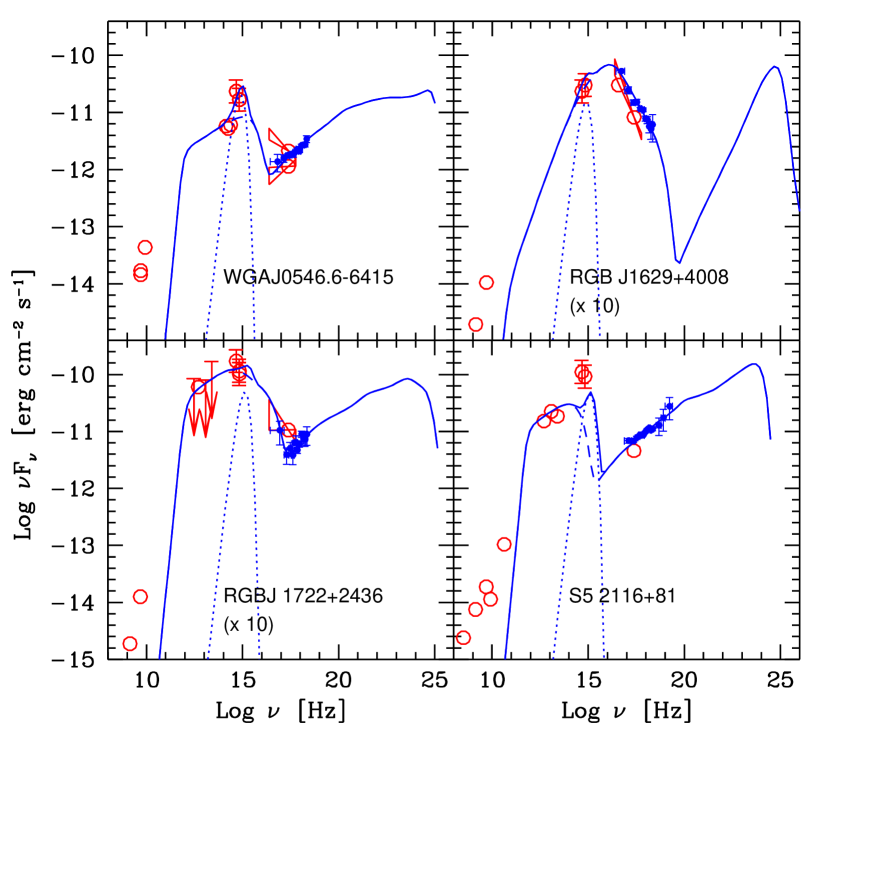
Figure 4: Spectral energy distributions of our sources. Open points represent data from the literature (NED) while the BeppoSAX data are indicated by filled points. ROSAT data are shown by a bow–tie that represents the spectral index range. The dashed lines correspond to the one–zone homogeneous synchrotron and inverse Compton model calculated as explained in the text, with the parameters listed in Table 10. Dotted lines represent the disk emission, while solid lines indicate the sum of disk plus non-thermal emission. The errors on the optical fluxes correspond to $\pm 0.5$ magnitudes (see text for details).

Table 10: Model Parameters.

Name	$L^{\prime}$	$L_{disk}$	$R_{BLR}$	$B$	$R$	$\Gamma$	$\theta$	$n$	$\gamma_{min}$	$\gamma_{peak}$	$\nu^{syn}_{peak}$	$B_{\rm eq}$
	erg s-1	erg s-1	cm	G	cm						Hz	G
WGA J0546.6$-$6415	2.5e42	1.4e46	2.7e18	1.0	8.0e15	12	3.5	3.6	3.0e1	1.0e4	5.8e15	3.2
RGB J1629$+$4008	3.0e41	7.2e44	3.5e17	2.5	1.0e16	13	3.0	4.2	1.0e4	1.0e4	1.7e16	0.9
RGB J1722$+$2436	1.3e42	9.3e44	4.0e17	4.0	7.0e15	13	5.0	3.5	1.0e2	1.5e3	3.8e14	2.7
S5 2116$+$81	2.0e42	1.9e45	7.0e17	1.0	1.0e16	11	5.0	3.5	2.0e1	3.0e3	3.9e14	2.3

We are aware of the fact that for three of our objects the shape, sampling, and lack of simultaneity of the SED do not allow us to firmly constrain the peak of the synchrotron emission (the exception being RGB J1629+4008), also because of the non-negligible contribution of the thermal disk component to the optical flux (especially for WGA J0546.6$-$6415 and S5 2116$+$81; see Fig. 4). However, some reasonable arguments can be made. For WGA J0546.6$-$6415 and RGB J1722$+$2436 the presence of a steeper (and variable) component at soft X-ray energies (§§ 4.5 and 5.4) may be attributed to the tail of the synchrotron emission (see also Sect. 7.2.3), thus suggesting a synchrotron peak which cannot be at too low energies ($\gtrsim 10^{14}$ Hz). This is corroborated also by the IR and optical data for RGB J1722$+$2436, whose optical flux is not dominated by the disk emission. In the case of WGA J0546.6$-$6415, which has a stronger disk component, the synchrotron peak could reach $\sim 10^{13}$ Hz only if one neglects the evidence for an upturn at low X-ray energies. S5 2116$+$81 is the less constrained source, but it is also the case for which we have no indication of a steep, soft X-ray component. The radio to IR data suggest a peak above $10^{13}$ Hz and no set of parameters was found to be compatible with the IR and BeppoSAX data and with a $\nu_{\rm peak}^{\rm syn}$ less than $\sim{\rm a~{}few}\times 10^{13}$ Hz. For all three objects, however, the synchrotron peak frequency has to be $<10^{16}$ Hz, since otherwise the X-ray band would have a strong and obvious steep synchrotron emission (as for RGB J1629$+$4008), contrary to what observed. In summary, we have modelled our objects mainly on the basis of the BeppoSAX (and partly ROSAT) data, trying to fit the other data as far as they could be compatible with the BeppoSAX ones. The derived parameters, then, apart from RGB J1629+4008, should be regarded as tentative.

The model fits are shown in Fig. 4 as solid lines. The applied model is aimed at reproducing the spectrum originating in a limited part of the jet, thought to be responsible for most of the emission. This region is necessarily compact, since it must account for the fast variability shown by all blazars, especially at high frequencies. The radio emission from this compact region is strongly self–absorbed, and the model cannot account for the observed radio flux. This explains why the radio data are systematically above the model fits in the figure. Our model fails also to reproduce the optical flux of S5 2116+81. This is the source with the lowest redshift ($z=0.084$) and we therefore expect a non–negligible contamination from the host galaxy, which is clearly detected in the Digitized Sky Survey (DSS) plates.

Note that the model fits predict that the high energy inverse Compton emission has a luminosity comparable to the synchrotron one in all sources but one, S5 2116+81. The shape of the inverse Compton component is sometimes complex, because of the contributions of the synchrotron self Compton component, especially in the X–ray range, and the external component, especially at higher energies.

As shown in Table 10, the intrinsic luminosities, the source dimensions, the bulk Lorentz factors and the viewing angles are quite similar for all sources. The fact that RGB J1629+4008 has a steep X–ray (synchrotron) spectrum is explained by our model by the very large value of $\gamma_{\rm min}$, the minimum Lorentz factor of the injected electrons which in this case corresponds to $\gamma_{\rm peak}$. The inferred values of the magnetic field are not very far from the equipartition values, with an average ratio $\langle B/B_{\rm eq}\rangle\sim 1.3$.

7 Discussion

Our source selection requires the objects to be in the HBL region and therefore to have relatively low $\alpha_{\rm ro}$ values. Given also their relatively low radio fluxes (and powers; see § 7.3), before discussing our results we need to assess if our sources are of the same kind as the more powerful and more studied blazars. We do this in the following subsection.

7.1 The Nature of Our Sources

7.1.1 Are our sources radio–loud?

Two different definitions of radio–loud quasars have been used in the literature (see, e.g., Stocke et al. 1992). The first is based on the rest–frame ratio $R$ of radio (typically 5 GHz) to optical (typically 4,400 Å) flux density, $\log R=\log(f_{\rm r}/{\rm mJy})+0.4B-6.66$ (independent of redshift if $\alpha_{\rm r}=\alpha_{\rm o}=0.5$ is assumed). Radio–loud sources are taken to have $R>10$ which translates, in our notation, to $\alpha_{\rm ro}\gtrsim 0.2$. The other definition is based on radio power and appears to be redshift-dependent, with a dividing line ranging from $\approx 10^{24}$ W Hz^-1 for the Palomar Green (PG) sample (optically bright and at relatively low-redshift) up to $10^{26}$ W Hz^-1 for the Large Bright Quasar Survey (LBQS) sample (optically fainter and at higher redshift). The two definitions overlap somewhat (Padovani, 1993). As shown in Fig. 2 and Tab. 1, all our sources are firmly in the radio-loud regime as far as the first definition is concerned. All of them have $\alpha_{\rm ro}\geq 0.26$, with $\langle\alpha_{\rm ro}\rangle\sim 0.33$ (or $\langle R\rangle\sim 50$; typical radio-quiet sources [i.e., optically selected quasars] have $\alpha_{\rm ro}\sim 0.1$ or $R\sim 0.5$). The 5 GHz radio powers of our sources are in the range $10^{24.6}-10^{26}$ W Hz^-1, with $\langle L_{\rm r}\rangle\sim 10^{25.1}$ W Hz^-1. Given their relatively low redshift ($\langle z\rangle\sim 0.2$), these values also classify our sources as radio-loud.

7.1.2 Are our sources blazars?

As described in the Introduction, blazars are characterized by a variety of properties, which have also led to a proliferation of names (HPQ, OVV, CDQ, FSRQ). The flat–spectrum radio quasar definition is the easiest one to apply, and it appears that the majority of powerful FSRQ indeed show rapid variability, high polarization, and radio structures dominated by compact radio cores, and vice versa (Urry & Padovani 1995 and references therein).

As our sources are less powerful than the FSRQ commonly studied (see § 7.2.4), it is important to check, as far as possible, that we are dealing with the same type of sources. We do this in the following.

Our objects have, by selection, a flat radio spectrum. In fact, $\langle\alpha_{\rm r}\rangle=-0.37$, that is their typical radio spectrum is not only flat but inverted. Three of our sources are included in the NVSS and therefore low-resolution (45^′′) radio maps at 1.4 GHz are available. RGB J1629$+$4008 and RGB J1722$+$2436 are compact and unresolved. RGB J1629$+$4008 is also included in the FIRST (Becker et al., 1995) radio survey, which has a higher resolution (5^′′) than the NVSS. This source is still compact and unresolved in the FIRST map, with a 1.4 GHz radio flux of $11.9\pm 0.2$ mJy, as compared to $9.0\pm 0.5$ mJy in the NVSS. The fact that the higher-resolution FIRST flux is similar to (actually larger than) the NVSS flux suggests that the source is core-dominated (modulo variability effects). S5 2116$+$81 has a complex NVSS map, with four radio sources within 3^′ from the source position. However, dedicated radio observations (Taylor et al., 1996) show that the VLA and VLBA (Very Long Baseline Array) 5 GHz core fluxes of the stronger source are basically the same, again indicating a very compact core. Finally, our own 4.8 and 8.6 GHz Australia Telescope Compact Array (ATCA) maps of WGA J0546.6$-$6415 (2^′′ and 1^′′ resolution, respectively) indicate a compact, unresolved source, with a core-dominance parameter at 4.8 GHz $\lesssim 35$ (see Landt et al. 2001 for details of the ATCA observations). The fact that the higher-resolution ATCA flux at 5 GHz is similar to (actually larger than) the lower-resolution Parkes-MIT-NRAO (PMN) (Wright et al., 1994) flux (339 mJy vs. 287 mJy) again suggests that the source is core-dominated (modulo variability effects).

Optical polarization data are available only for two of our sources, RGB J1722$+$2436 and S5 2116$+$81. The former has $P_{\rm opt}=0.70\pm 0.48$% (Stockman, Moore, & Angel, 1984) while the latter has $P_{\rm opt}=0.94\pm 0.21$% (Marchã et al., 1996). We note that although these values are below the “canonical” division between high-polarized (HPQ) and low-polarized (LPQ) quasars (and are indeed not inconsistent with possible scattering by the interstellar medium of our own galaxy), many flat–spectrum LPQ are also thought to be seen with their jets at small angles w.r.t. the line of sight (e.g., Ghisellini et al. 1993), and therefore classify as “blazars” according to our definition. Furthermore, if indeed these objects are the equivalent to HBL, as discussed in § 7.2, we would expect their duty-cycle for high polarization to be lower than their low-frequency peaked relatives, as was found for HBL and LBL by Jannuzi, Smith, & Elston (1994). Finally, the relative prominent thermal emission, especially in S5 2116$+$81 (see Fig. 4), would also explain a low optical polarization.

As regards variability, at least three of our sources appear to vary in the X–ray band, based on our BeppoSAX and ROSAT comparison, with RGB J1629+4008 decreasing in flux by a factor of 4 in 7 hours in our MECS and LECS observations.

7.2 Have we found high-frequency peaked FSRQ?

The purpose of this paper was to study the X–ray properties and, more generally, the SED of a class of flat–spectrum radio quasars with relatively large X–ray–to–radio flux ratios and effective spectral indices typical of HBL. We now address the question if these sources are really the strong, broad-lined counterparts of HBL.

7.2.1 Spectral Energy Distributions

The SED of RGB J1629+4008 is HBL–like, with the steep X–ray spectrum clearly attributable to synchrotron emission. For WGA J0546.6$-$6415 and RGB J1722+2436 the situation is less clear. Our fits and the SEDs are not inconsistent with the fact that the BeppoSAX band might be close to the “valley” between synchrotron and inverse Compton emission, which would classify them as akin to “intermediate” BL Lacs. Finally, S5 2116+81 appears to be LBL–like.

7.2.2 X–ray spectral index and the synchrotron peak frequency

A good indicator of the dominant emission process in the X–ray band is the X–ray spectral index – synchrotron peak frequency plot (Padovani & Giommi, 1996; Lamer, Brunner, & Staubert, 1996). Padovani & Giommi (1996) found a strong anti–correlation between the ROSAT $\alpha_{\rm x}$ and $\nu_{\rm peak}$ for HBL (i.e., the higher the peak frequency, the flatter the spectrum), while basically no correlation was found for LBL. This was interpreted as due to the tail of the synchrotron component becoming increasingly dominant in the ROSAT band as $\nu_{\rm peak}$ moves closer to the X–ray band (see Fig. 7 of Padovani & Giommi 1996).

The BeppoSAX version of this dependence was studied by Padovani et al. (2001; see their Fig. 7). They confirmed the ROSAT findings, namely a strong anti-correlation between $\alpha_{\rm x}$ and $\nu_{\rm peak}$ for HBL and no correlation for LBL, with an initial increase in $\alpha_{\rm x}$ going from LBL to HBL (see Padovani et al. 2001 for details).

The BeppoSAX spectral index ($0.1-10$ keV) versus the logarithm of the synchrotron peak frequency for our sources (filled circles), HBL (crosses), and LBL (open circles). Data for LBL come from Padovani et al. (2001), while those for HBL come from Wolter et al. (1998; updated in Beckmann et al. 2002), Beckmann et al. (2002), and Padovani et al. (2001). Three of our sources, namely those with values of $\alpha_{\rm x}<1$, have quite uncertain $\nu_{\rm peak}$ values but likely in the range $10^{14}\lesssim\nu_{\rm peak}<10^{16}$ Hz (see text for details).

Fig. 7.2.2 shows an updated version of the $\alpha_{\rm x}-\nu_{\rm peak}$ plot for BL Lacs from Padovani et al. (2001), including the HBL studied by Beckmann et al. (2002). We have also included in this plot our sources, represented by filled points. We notice that RGB J1629+4008 falls right in the region occupied by HBL, again confirming our interpretation that its BeppoSAX band is dominated by synchrotron emission. This is further supported by the detection of rapid variability, which has been seen in the synchrotron emission of several BL Lacs observed with BeppoSAX but never in the inverse Compton component, which varies on much longer time scales (e.g, Ravasio et al. (2002) and references therein). The other three sources have values which, although quite uncertain, are probably in the range $10^{14}\lesssim\nu_{\rm peak}<10^{16}$ Hz, which overlap with the values typical of “intermediate” BL Lacs, but display relatively flat $\alpha_{\rm x}$. We notice that the scatter in the diagram is larger in the $\nu_{\rm peak}$ range $\approx 10^{14}-10^{15.5}$ Hz, which is also where the HBL/LBL division becomes blurrier. We interpret this as due to the fact that in this range of $\nu_{\rm peak}$ objects can be both synchrotron and inverse Compton dominated, depending on variability state. For comparison, note that 3C 279, a classical FSRQ, has a BeppoSAX spectral index $\alpha_{\rm x}=0.66\pm 0.04$ and $\nu_{\rm peak}\sim 10^{13}$ Hz (Ballo et al., 2002), i.e., well into the LBL region.

7.2.3 The “Blue Bump” Component

Fig. 4 shows that the thermal component is non–negligible in most of our sources, with a ratio of black–body to synchrotron emission at $\sim 5,000$ Å ranging from $\sim 2$ for WGA J0546.6$-$6415 and S5 2116$+$81 to $\sim 0.2$ for RGB J1722$+$2436. While these ratios are model–dependent, especially for the former sources for which the optical band is close to the synchrotron cut–off, it is instructive to check the effect of the thermal component on the position of our objects in the $\alpha_{\rm ro}-\alpha_{\rm ox}$ plane. By subtracting the thermal component and therefore using only the synchrotron flux in the optical band to derive effective spectral indices, we can see where the objects would fall (we assume that the blue bump has no effect at 1 keV; but see below). As $\alpha_{\rm rx}$ stays constant while $\alpha_{\rm ro}$ and $\alpha_{\rm ox}$ get steeper and flatter respectively, the sources move along diagonal lines up and to the left in the diagram. More specifically, the “synchrotron only” values are as follows: WGA J0546.6$-$6415, $\alpha_{\rm ro}\sim 0.5$, $\alpha_{\rm ox}\sim 1$, RGB J1629$+$4008, $\alpha_{\rm ro}\sim 0.4$, $\alpha_{\rm ox}\sim 0.85$, S5 2116$+$81, $\alpha_{\rm ro}\sim 0.4$, $\alpha_{\rm ox}\sim 1.2$ (practically no change is required for RGB J1722$+$2436). It then follows that even by subtracting the effect of the thermal component our sources would still be well within the HBL region in the $\alpha_{\rm ro}-\alpha_{\rm ox}$ plane (Fig. 2). Actually, the effect of a strong blue bump, by moving sources to the right and down in the diagram, is that of “pushing” objects off the HBL region and into the radio-quiet zone. Even with some freedom in the modelling of the synchrotron component, the location of our sources in the HBL region results quite robust, and cannot be ascribed to the accretion disk. That relatively high values of $\nu_{\rm peak}$ are not due to the accretion disk is also indicated by the low, “HBL–like” values of $\alpha_{\rm rx}$, a parameter well correlated with $\nu_{\rm peak}$ (e.g., Padovani & Giommi 1996) and not affected by the optical contamination. Note that the $\nu_{\rm peak}$ values given in Tab. 10 and shown in Fig. 7.2.2 are those relative only to the synchrotron component and therefore do not include the thermal component.

In Seyfert galaxies and radio–quiet quasars the X–ray emission is thought to be produced by a hot thermal corona sandwiching a relatively cold accretion disk. One could then ask if the same component can contribute also in our objects, two of which indeed have a relatively large disk component in the optical–UV band. While it is certainly possible that some fraction of the X–ray emission (especially at low energies) is produced by a hot corona, we believe that the non–thermal components in these objects are dominant, due to the X-ray variability indicated by the comparison between BeppoSAX and ROSAT data, particularly the rapid LECS/MECS variability seen in RGB J1629+4008, and to the lack of any indication of iron line features and hardening of the spectrum due to the so–called Compton hump (which are instead common in Seyfert galaxies). A possible way to decrease the importance of the iron line emission and Compton hump in the spectrum could be to assume a dynamic corona, but in such case the corona emission would be characterized by harder X-ray spectra ($\alpha_{\rm x}<1$; see Malzac et al. 2001), and thus could not account for soft excesses or steep spectra.

7.2.4 Source Powers

As discussed above, the 5 GHz radio powers of our sources are in the range $10^{24.6}-10^{26}$ W Hz^-1, with $\langle L_{\rm r}\rangle\sim 10^{25.1}$ W Hz^-1. Their 1 keV X–ray powers are in the range $10^{19.4}-10^{20.6}$ W Hz^-1, with $\langle L_{\rm x}\rangle\sim 10^{20.1}$ W Hz^-1. These values, although not very different from the mean values of the EMSS BL Lacs ($\langle L_{\rm r}\rangle\sim 10^{24.8}$ W Hz^-1 and $\langle L_{\rm x}\rangle\sim 10^{20.3}$ W Hz^-1), are still in the FSRQ range, albeit on the low side (see, for example, Fig. 5 of Perlman et al. 1998 and Padovani et al., in preparation). Their radio powers put our sources near the low–luminosity end of the DXRBS FSRQ radio luminosity function (Padovani, 2001).

7.3 Astrophysical Interpretation

We have found three examples of strong, broad–lined blazars with an SED typical of HBL (one source) and intermediate BL Lacs (two sources). While the first case is quite strong, the other two are more tentative. These are the first such sources, as most broad–lined blazars known so far have SED typical of LBL, i.e., with synchrotron peaks at IR/optical energies.

Our FSRQ, however, have relatively low powers, more typical of BL Lacs than quasars. This ties in with the suggestion by Ghisellini et al. (1998) and Ghisellini, Celotti, & Costamante (2002) that blazars form a sequence, controlled mainly by their bolometric luminosity which in turn controls the amount of cooling suffered by the emitting electrons. In powerful sources, where cooling is severe (high radiative ($U_{\rm r}$) plus magnetic field ($U_{\rm B}$) energy densities), electrons of all energies cool rapidly (i.e., in a time shorter than the injection time), making the particle distribution to have a break at $\gamma=\gamma_{\rm min}$, which in this case becomes $\gamma_{\rm peak}$. These sources are typically LBL–like, and are those located in the lower part of the $\gamma_{\rm peak}-U_{\rm r}+U_{\rm B}$ plot (see Fig. 7.3). In less powerful sources, instead, only the highest energy electrons can cool in the injection time, and consequently the particle distribution will have a break at $\gamma=\gamma_{\rm c}$, for which $t_{\rm cool}=t_{\rm inj}$. In this case $\gamma_{\rm peak}=\gamma_{\rm c}$ (and $\propto(U_{\rm r}+U_{\rm B})^{-1}$; see details in Ghisellini, Celotti, & Costamante (2002)). Fig. 7.3 shows that the FSRQ studied in this paper, which have relatively high $\gamma_{\rm peak}$ (and therefore $\nu_{\rm peak}$) values, appear to fit within this scenario, as they follow the suggested sequence. (Note that, given the scatter in the plot, this conclusion stands even in the case of a decrease of $\sim$ one order of magnitude in the $\gamma_{\rm peak}$ values for the three sources with relatively uncertain estimates of this parameter.) Moreover, in agreement with their relatively low powers, they are positioned at the low-end of the FSRQ region and actually within the BL Lac region. In other words, we still have not found a case of high–$\nu_{\rm peak}$ (and therefore high–$\gamma_{\rm peak}$) and high–power blazar, which would invalidate this scenario.

$\gamma_{\rm peak}$, the Lorentz factor of the electrons emitting most of the radiation, vs. the total energy density in the emitting region, i.e., the sum of the radiative ($U_{\rm r}$) and magnetic field ($U_{\rm B}$) energy densities, as measured in the comoving frame. Open circles represent “extreme” HBL, filled circles represent TeV sources, open squares represent BL Lacs, open triangles represent FSRQ, filled triangles are FSRQ at $z>4$, while stars indicate our sources (HFSRQ). All data apart from the latter are from Ghisellini, Celotti, & Costamante (2002), updated in part from Ghisellini et al. (1998).

Another explanation for the relatively low power of our sources is related to a selection effect. Fig. 4 shows that our only “true” HBL–like FSRQ, RGB J1629$+$4008, has a synchrotron peak at $\sim 2\times 10^{16}$ Hz, well above the peak of the thermal emission. Its non-thermal power is also low enough (as implied by its radio power $L_{\rm 5GHz}\sim 6\times 10^{24}$ W Hz^-1) that the thermal component, and its associated broad lines, is non–negligible in the optical/UV band. Given that the equivalent width of its strongest emission line is $\sim 80$ Å, the same object with a non-thermal power a factor of $\sim 20$ higher, corresponding to $L_{\rm 5GHz}\sim 10^{26}$ W Hz^-1, still rather modest for an FSRQ, would be classified as a BL Lac object, since its equivalent width would go down to $\sim 4$ Å. An even stronger non-thermal component would completely wash out the emission lines, making the redshift determination of this object impossible, as there are no galaxy absorption features in its spectrum. It then follows that a broad-lined source with the same SED as RGB J1629$+$4008 but a much larger power would not even be classified as an FSRQ but as an HBL without redshift. This could also explain why high–power, high–$\nu_{\rm peak}$ BL Lacs have not been yet found. A key ingredient of this argument is the frequency of the synchrotron peak. Assuming a typical $\nu_{\rm peak}$ value for a “classical” FSRQ of $\sim 10^{13.5}$ Hz, which implies a much weaker optical synchrotron component, an object with a radio power $\sim 100$ times larger than RGB J1629$+$4008 will have the same optical (non-thermal) power and therefore will still be recognized as a quasar (assuming similar thermal powers). It follows that high–power, low–$\nu_{\rm peak}$ FSRQ can be identified as quasars up to very high luminosities. Conversely, high–$\nu_{\rm peak}$ blazars would be classified as HBL without redshift already at moderate radio luminosities. One problem with this explanation for the lack of high–$\nu_{\rm peak}$ — high–power blazars is that there should be intermediate cases, i.e., HBL with broad (but weak) lines. This does not seem apparent, for example, from the optical spectra of the EMSS BL Lacs (e.g., Rector et al. 2000).

As the selection of our sources was done $3-4$ years ago, one could ask if our sources are still really extreme in terms of their X–ray–to–radio flux ratios. Out of the 199 DXRBS FSRQ known to date, WGA J0546.6$-$6415 is still the second most extreme. The FSRQ RGB sample, given its higher X–ray flux limit and slightly lower radio flux limit, is even better suited to find sources with high $f_{\rm x}/f_{\rm r}$ ratios (lower $\alpha_{\rm rx}$; see Padovani et al., in preparation). Sorting the known RGB FSRQ in order of ascending $\alpha_{\rm rx}$ value, RGB J1629$+$4008 is at the top of the list while RGB J1722$+$2436 is number four (RGB J1413+4339, which is number two, is a borderline quasar; see Laurent-Muehleisen et al. 1998). Finally, S5 2116$+$81 is number 15 out of the $\sim 400$ FSRQ in the multifrequency catalog of Padovani, Giommi, & Fiore (1997) with X–ray data sorted in order of ascending $\alpha_{\rm rx}$ value. It was selected because it is the X–ray brightest.

We find it significant that, having selected some of the few known FSRQ with effective spectral indices typical of HBL and therefore relatively large X–ray–to–radio flux ratios, we found only one case where the X–ray band is clearly dominated by synchrotron emission, with a $\nu_{\rm peak}\sim 2\times 10^{16}$ Hz, while the other three sources have $\langle\nu_{\rm peak}\rangle\lesssim 10^{15}$ Hz. As shown, for example, in Fig. 7.2.2, HBL can reach much higher values, up to $10^{18}-10^{19}$ Hz, albeit in cases of extreme variability (e.g., MKN 501; Pian et al. 1998). A more meaningful comparison is with the HBL in the multifrequency catalog of Padovani, Giommi, & Fiore (1997) having radio flux $>20$ mJy, the minimum value for our sources. In that case the $\nu_{\rm peak}$ distribution has a typical value $\sim 4\times 10^{16}$ Hz and reaches $\sim 2\times 10^{17}$ Hz. A discussion of the $\nu_{\rm peak}$ distribution for FSRQ and BL Lacs belonging to the same sample will be presented by Padovani et al. (in preparation).

Sambruna, Chou, & Urry (2000) reported on ASCA observations of four FSRQ characterized by steep ROSAT spectra ($\alpha_{\rm x}\sim 1.3$). The sources were all found to have flat hard X–ray spectra, with $\alpha_{\rm x}\sim 0.8$. Sambruna et al. discuss their results in terms of relatively high synchrotron peaks and thermal emission extending into the X–ray band. We stress, however, that their sources sample a region of parameter space widely different from ours. Their effective spectral indices, in fact, place their FSRQ firmly in the LBL region, unlike ours, so that their four objects should not have been expected to show high $\nu_{\rm peak}$ values and steep ASCA spectra. Georganopoulos (2000) used the fact that these four FSRQ happen to have relatively low core-dominance parameters ($\approx 1$) compared to two “intermediate” BL Lacs to suggest that these sources could be seen at larger angles than more typical FSRQ. We stress that, as discussed in § 7.1.2, our sources, and especially RGB J1629+4008, appear to be quite compact so that his interpretation might not apply to our objects.

8 Summary and Conclusions

We have presented new BeppoSAX observations of four flat–spectrum radio quasars selected to have effective spectral indices ($\alpha_{\rm ro}$, $\alpha_{\rm ox}$) typical of high-energy peaked BL Lacs. The main purpose of the paper was to see if these sources are indeed the broad-lined counterparts of BL Lacs with the synchrotron peak at UV/X–ray energies (HBL). Our objects are quite extreme in terms of their X–ray–to–radio flux ratios (a factor $\sim 70$ higher than “classical” FSRQ), qualify as radio-loud sources both in terms of their radio-to-optical flux ratio and power, and are variable and radio-compact. Our main results can be summarized as follows:

1. We have discovered the first FSRQ (RGB J1629+4008) whose X–ray emission is dominated by synchrotron radiation, as clearly shown by our BeppoSAX observations ($\alpha_{\rm x}\sim 1.5$ in the $0.1-10$ keV band), in which the source was also rapidly variable. This object is therefore the first confirmed member of a newly established class of HBL–like FSRQ. This result is fully consistent with earlier ROSAT observations which detected a steep soft X–ray spectrum ($\alpha_{\rm x}\sim 2$ in the $0.1-2.4$ keV band). The combination of the X–ray data with archival radio and optical data gives a spectral energy distribution typical of HBL sources, with a synchrotron $\nu_{\rm peak}\sim 2\times 10^{16}$ Hz. The derived values follow very well the $\alpha_{\rm x}-\nu_{\rm peak}$ correlation seen for HBL sources (Fig. 7.2.2).

2. The other three sources show a relatively flat ($\alpha_{\rm x}\sim 0.75$) BeppoSAX spectrum. However, we have found for two of them (WGA J0546$-$6415 and RGB J1722+2436) some indication of steepening at low-energies. This is based on BeppoSAX and ROSAT data and on their (sparsely sampled) SEDs. We interpret this as the tail of synchrotron emission, which is not strongly constrained but would peak around $\approx 10^{15}$ Hz, as typical of “intermediate” BL Lacs for which the synchrotron and inverse Compton components meet within the BeppoSAX band. The last source (S5 2116+81) turned out to be a more typical FSRQ, with the BeppoSAX band fully dominated by inverse Compton emission and a synchrotron $\nu_{\rm peak}<10^{15}$ Hz.

3. By fitting a synchrotron inverse Compton model which includes the contribution of an accretion disk, whose power we estimate from the broad-line region luminosity, to the spectral energy distributions, we have derived physical parameters (e.g., intrinsic power, magnetic field, etc.) for our sources. The thermal component was found to be non-negligible in three out of four objects, with ratios of thermal to synchrotron emission in the range $0.6-2$ at 5,000 Å.

4. Although the original selection was based mostly on the effective broad-band (radio through X–ray) colors, which are in first approximation independent of luminosity, all four candidates are at relatively low powers, more typical of BL Lacs than of FSRQ and in any case close to the low-luminosity end of the FSRQ radio luminosity function (Padovani, 2001). We interpret this as due to two, possibly concurrent, causes: an inverse dependence of $\gamma_{\rm peak}$ (and therefore $\nu_{\rm peak}\propto\gamma_{\rm peak}^{2}\delta B$), the Lorentz factor of the electrons emitting most of the radiation, on bolometric power, due to the more sever cooling at work in more powerful sources; and a selection effect, namely the fact that a high-power, HBL–like quasar will have such a strong optical/UV non-thermal component that its emission lines will be swamped and the object will be classified as a featureless BL Lac.

A better understanding of these rare sources and the confirmation of the non-existence of high–$\nu_{\rm peak}$ — high–power blazars will require the selection and study of a larger sample of objects.

References

- Ballo et al. (2002) Ballo, L., et al. 2002, ApJ, 567, 50
- Balucinska-Church & McCammon (1992) Balucinska-Church, M., & McCammon, D. 1992, ApJ, 400, 699
- Becker et al. (1995) Becker, R. H., White, R. L., & Helfand, D. J. 1995, ApJ, 450, 559
- Beckmann et al. (2002) Beckmann, V., Wolter, A., Celotti, A., Costamante, L., Ghisellini, G., Maccacaro, T., & Tagliaferri, G. 2002, A&A, 383, 410
- Boella et al. (1997a) Boella, G., et al. 1997a, A&AS, 122, 299
- Boella et al. (1997b) Boella, G., et al. 1997b, A&AS, 122, 327
- Bond et al. (1977) Bond, H. E., Kron, R. G., & Spinrad, H. 1977, ApJ, 213, 1
- Brinkmann et al. (1997) Brinkmann, W., et al. 1997, A&A, 323, 739
- Celotti, Padovani, & Ghisellini (1997) Celotti, A., Padovani, P., & Ghisellini. G. 1997, MNRAS, 286, 415
- Condon et al. (1998) Condon, J. J., Cotton, W. D., Greisen, E. W., Yin, Q. F., Perley, R. A., Taylor, G. B., & Broderick, J. J. 1998, AJ, 115, 169
- Cutri et al. (2000) Cutri, R. M., et al. 2000, Explanatory Supplement to the 2MASS Second Incremental Data Release, available at: http://www.ipac.caltech.edu/2mass/releases/second/doc/explsup.html
- De Grandi & Molendi (2002) De Grandi, S. & Molendi, S. 2002, ApJ, 567, 163
- Dickey & Lockman (1990) Dickey, J. M. & Lockman, F. J. 1990, ARA&A, 28, 215
- Fiore et al. (1999) Fiore, F., et al. 1999, Handbook for NFI Spectral Analysis, available at: http://www.asdc.asi.it/bepposax/software/
- Fossati et al. (1998) Fossati, G., Maraschi, L., Celotti, A., Comastri, A., & Ghisellini, G. 1998, MNRAS, 299, 433
- Frontera et al. (1997) Frontera, F., et al. 1997, A&AS, 122, 357
- Georganopoulos (2000) Georganopoulos, M. 2000, ApJ, 543, L15
- Ghisellini et al. (1998) Ghisellini, G., Celotti, A., Fossati, G., Maraschi, L., & Comastri, A. 1998, MNRAS, 301, 451
- Ghisellini, Celotti, & Costamante (2002) Ghisellini, G., Celotti, A., & Costamante, L. 2002, A&A, 386, 763
- Giommi & Fiore (1997) Giommi, P., & Fiore, F. 1997, in Proc. 5th International Workshop on Data Analysis in Astronomy (Singapore: World Scientific), 93
- Giommi & Padovani (1994) Giommi, P., & Padovani, P. 1994, MNRAS, 268, L51
- Giommi et al. (1999) Giommi, P., et al. 1999, A&A, 351, 59
- Giommi et al. (2000) Giommi, P., Padovani, P., & Perlman, E. 2000, MNRAS, 317, 743
- Haardt et al. (2001) Haardt, F., et al. 2001, ApJS, 133, 187
- Haberl & Pietsch (1999) Haberl, F., & Pietsch, W. 1999, A&AS, 139, 277
- Hambly et al. (2001) Hambly, N. C. et al. 2001, MNRAS, 326, 1279
- Helfand et al. (2001) Helfand, D. J., Stone, R. P. S., Willman, B., White, R. L., Becker, R. H., Price, T., Gregg, M. D., & McMahon, R. G. 2001, AJ, 121, 1872
- Irwin et al. (1994) Irwin, M., Maddox, S., & McMahon, R. 1994, Spectrum, 2, 14
- Iwasawa, Fabian, & Nandra (1999) Iwasawa, K., Fabian, A. C., & Nandra, K. 1999, MNRAS, 307, 611
- Jannuzi, Smith, & Elston (1994) Jannuzi, B. T., Smith, P. S., & Elston R. 1994, ApJ, 428, 130
- Kaspi et al. (2000) Kaspi, S., Smith, P. S., Netzer, H., Maoz, D., Jannuzi, B. T., & Giveon, U. 2000, ApJ, 533, 631
- Kollgaard (1994) Kollgaard, R. I. 1994, Vistas Astron., 38, 29
- Lamer, Brunner, & Staubert (1996) Lamer, G., Brunner, H., & Staubert, R. 1996, A&A, 311, 384
- Landt et al. (2001) Landt, H., Padovani, P., Perlman, E. S., Giommi, P., Bignall, H., & Tzioumis, A. 2001, MNRAS, 323, 757
- Laurent-Muehleisen et al. (1998) Laurent-Muehleisen, S. A., Kollgaard, R. I., Ciardullo, R., Feigelson, E. D., Brinkmann, W., & Siebert, J. 1998, ApJS, 118, 127
- Malzac et al. (2001) Malzac, J., Beloborodov, A.M., & Poutanen, J. 2001, MNRAS, 326, 417
- Marchã et al. (1996) Marchã, M. J. M., Browne, I. W. A., Impey, C. D., & Smith, P. S. 1996, MNRAS, 281, 425
- Mineo et al. (2000) Mineo, T., et al. 2000, A&A, 359, 471
- Morrison & McCammon (1983) Morrison, R., & McCammon, D. 1983, ApJ, 270, 119
- Padovani (1992) Padovani, P. 1992, MNRAS, 257, 404
- Padovani (1993) Padovani, P. 1993, MNRAS, 263, 461
- Padovani & Giommi (1995) Padovani, P., & Giommi, P. 1995, ApJ, 444, 567
- Padovani & Giommi (1996) Padovani, P., & Giommi, P. 1996, MNRAS, 279, 526
- Padovani, Giommi, & Fiore (1997) Padovani, P., Giommi, P., & Fiore, F. 1997, in From the Micro- to the Mega-Parsec, ed. A. Comastri, T. Venturi, & M. Bellazzini, MmRAS, 68, 147
- Padovani (2001) Padovani, P. 2001, in ASP Conf. Ser. 227, Blazar Demographics and Physics, ed. P. Padovani, & C. M. Urry, 163
- Padovani et al. (2001) Padovani, P., et al. 2001, MNRAS, 328, 931
- Parmar et al. (1997) Parmar, A., et al. 1997, A&AS, 122, 309
- Perlman et al. (1998) Perlman, E. S., Padovani, P., Giommi, P., Sambruna, R., Jones, L. R., Tzioumis, A., & Reynolds, J. 1998, AJ, 115, 1253
- Perlman et al. (1996) Perlman, E. S., Stocke, J. T., Morris, S. L., & Wang, Q. D. 1996, ApJ, 456, 451
- Pian et al. (1998) Pian, E., et al. 1998, ApJ, 492, L17
- Ravasio et al. (2002) Ravasio, M. et al. 2002, A&A, 383, 763
- Rector et al. (2000) Rector, T. A., Stocke, J. T., Perlman, E. S., Morris, S. L., & Gioia, I. M. 2000, AJ, 120, 1626
- Sambruna, Maraschi & Urry (1996) Sambruna, R., Maraschi, L., & Urry, C. M. 1996, ApJ, 463, 444