The Structure and X-ray Recombination Emission of a Centrally Illuminated Accretion Disk Atmosphere and Corona

Abstract

We model an accretion disk atmosphere and corona photoionized by a central X-ray continuum source. We calculate the opacity and one-dimensional radiation transfer for an array of disk radii, to obtain the two-dimensional structure of the disk and its X-ray recombination emission. The atmospheric structure is extremely insensitive to the viscosity $\alpha$. We find a feedback mechanism between the disk structure and the central illumination, which expands the disk and increases the solid angle subtended by the atmosphere. We apply the model to the disk of a neutron star X-ray binary. The model is in agreement with the $\sim 12\hbox{${}^{\circ}$}$ disk half-angle measured from optical light curves. We map the temperature, density, and ionization structure of the disk, and we simulate high resolution spectra expected from the Chandra and XMM-Newton grating spectrometers. X-ray emission lines from the disk atmosphere are detectable, especially for high-inclination binary systems. The grating observations of two classes of X-ray binary systems already reveal important spectral similarities with our models. The model spectrum is dominated by double-peaked lines of H-like and He-like ions, plus weak Fe L. The line flux is proportional to the luminosity and is dominated by the outer radii. Species with a broad range of ionization levels coexist at each radius: from Fe XXVI in the hot corona, to C VI at the base of the atmosphere. The line spectrum is very sensitive to the temperature, ionization, and emission measure of each atmospheric layer, and it probes the heating mechanisms in the disk. We assume a hydrostatic disk dominated by gas pressure, in thermal balance, and in ionization equilibrium. As boundary conditions, we take a Compton-temperature corona and an underlying Shakura-Sunyaev disk. The choice of thermally stable solutions strongly affects the spectrum, since a thermal instability is present in the regime where X-ray recombination emission is most intense.

1 Introduction

When the infall of matter into a deep gravitational potential is mediated by an accretion disk, gravitational energy is converted to the thermal radiation which powers both low mass X-ray binary (LMXB) systems and active galactic nuclei (AGN). Accretion disks present unique problems involving magnetized plasma dynamics, photoionization, atomic kinetics, thermal and ionization equilibria, general relativity, and radiation transfer. The accretion disks in LMXBs and AGN are expected to have many common properties. The compactness of the accretor in LMXBs and AGN and their inferred accretion rates imply temperatures of $T>10^{7}$ K and intense X-ray emission in the inner disk region. The inner radii of these disks, as well as the disk atmosphere as a whole, is substantially more ionized than the case in which the accretor is a white dwarf. In both LMXBs and AGN, the vast energy emitted in the inner disk region is reprocessed in the outer disk, where the external radiative heating can dominate the local thermal emission. The subsequent photoionization of the disk plasma radically alters its equilibrium state, structure, and spectrum, especially in the atmospheric and coronal disk layers, which are the subject of this study.

High resolution X-ray spectroscopy is an essential tool to study the physics of this ”hot class” of accretion disks and the conditions near black hole event horizons. In this paper, we concentrate on the outer radii of disks in neutron star LMXBs, since current observational constraints provide more stringent tests for LMXBs than for AGN. The following points support these assertions:

• High resolution spectra can reveal discrete emission or absorption from atomic transitions within the accretion disk plasma, providing information on the accretion disk structure, dynamics, and physics. These spectra open a window into photoionized gases and their phase equilibria.

• X-rays, and in particular discrete atomic transitions of hydrogen- and helium-like ions, probe the regions in the disk with the highest levels of ionization. Regions closer to the compact object will have the highest ionization levels, although vertical stratification is also expected.

• The knowledge of the accretion disk physics directly impacts our ability to probe the physical conditions around the compact object. For example, the Fe K emission originating in the innermost regions of an accretion disk has been proposed as a direct probe of the general relativistic effects near a black hole event horizon in AGN, by virtue of the observed characteristic line shape (Tanaka et al., 1995). However, very little is known about the physical conditions in the Fe K emission region, and it is still unclear how our ignorance of the physical processes within the accretion disk affect the modeled Fe K line profile and flux. It is also unclear whether the soft X-ray line features reported by Branduardi-Raymont et al. (2001) are feasible.

• While in neutron star LMXBs the photoionizing source must be near the neutron star surface, in AGN and galactic black hole candidates (BHC) the location of the ionizing source is unknown. In AGN, various authors have assumed the ionizing source to be located in the rotation axis of the black hole, above the disk midplane, possibly close to the base of a jet. Alternatively, an ionizing source might be present on the upper layers of the disk, perhaps due to disk flares, or to Comptonization of thermal UV photons in the accretion disk corona (ADC).

• LMXB systems are observed in less crowded regions than AGN.

• In contrast to AGN, LMXBs often have measured orbital parameters which constrain the geometry of the system, such as the maximum disk radius. LMXBs may also have a measured value of the disk inclination, while orbital phase and eclipse phase variations provide tomographic information. For example, measurements of the optical light curve amplitudes of LMXBs have yielded estimates of the angle subtended by the disk of $\sim$ 12^∘ (de Jong, van Paradijs, & Augusteijn, 1996).

• To our knowledge, the inner disk radii can only be studied in the X-ray band. Theoretically, the thermal emission of the inner disk radii must peak in the X-ray band for both LMXBs and AGN. The optical and UV emission originates in the outer regions of the accretion disk and further away from the compact object, and the radio and gamma ray emission is likely dominated by emission from jets.

Fewer physical ingredients are needed to model the outer radii of disks than the inner radii, so the logical progression is to successfully model the outer radii first. The X-ray spectroscopy of neutron star LMXBs will allow us to construct a physical picture of their accretion disks, which we can then use to investigate the inner disk in BHC and AGN.

To fully exploit the high energy-resolution X-ray spectra of accretion disks, we created physical disk models and calculated synthetic spectra. The disk plasma, at $10^{5}$ to $10^{7}$ K, cools through atomic line emission that can be detected with space-borne X-ray observatories such as Chandra and XMM-Newton. Modeling the equilibrium state of the plasma and the radiation transfer within the disk allows a calculation of the disk structure and its X-ray spectrum. A synthetic spectrum can be compared to the data. The model spectrum is unique in that it is calculated purely on physical, and not just phenomenological, grounds.

We describe four fiducial disk models. Two of these models were introduced in Jimenez-Garate, Raymond, Liedahl, & Hailey (2001). We use a newly developed adaptive-mesh disk structure calculation, the Raymond (1993) photoionized plasma code, and a new X-ray emission code which uses $HULLAC$ data (Hebrew University/Lawrence Livermore Atomic Code, Klapisch et al. (1977)). The models consist of a disk illuminated by a pure neutron star continuum, and they contain as boundary conditions a Compton-temperature ADC at the top of the disk and a modified Shakura & Sunyaev (1973, hereafter abbreviated as SS73) disk at the bottom (Vrtilek et al., 1990). Thus, the region of interest has a temperature and ionization which is intermediate of these two regions, and it emits copious X-ray radiation.

In section 2.1, we introduce the X-ray line observations prior to Chandra and XMM-Newton; in section 2.2, we introduce theoretical work on the structure of X-ray illuminated accretion disks; in section 3, we describe the disk structure calculations and the assumptions of hydrostatic, thermal and ionization equilibrium; in section 4, we detail the effects of a thermal instability on a layer of the disk atmosphere throughout the disk; in section 5, we discuss the calculation of the high resolution spectrum, which is done a posteriori from the structure calculation; in section 6, the disk density, temperature and ionization structure are presented; in section 7, the model spectra are shown, assuming a full, partial or obstructed view of the neutron star region, and we show simulated spectra utilizing the response of the XMM-Newton reflection grating spectrometer (RGS) and the Chandra medium energy gratings (MEG); in section 8, comparisons of the model to the observed X-ray spectra of LMXBs are discussed briefly, and we discuss the limitations of the model. In section 9, concluding remarks are presented.

2 LMXB accretion disks

2.1 X-ray line emission from LMXBs

With the exception of Fe K emission in the 6.4–7.0 keV range (Asai, Dotani, Nagase, & Mitsuda, 2000), discerning X-ray line emission in LMXBs has been challenging, owing to limitations in sensitivity and spectral resolving power, as well as the difficulties associated with attempts to extract line emission from data dominated by intense continuum emission. Measurements obtained with the Einstein Objective Grating Spectrometer (Vrtilek et al., 1991), the ROSAT Position Sensitive Proportional Counter (Schulz, 1999), and the ASCA CCD imaging detectors (Asai, Dotani, Nagase, & Mitsuda, 2000) have shown that the spectra of a large fraction of bright LMXBs exhibit line emission. X-ray lines at $\sim 1$ keV are often mixed with various species, so that only the brightest LMXBs had clear line identifications, as in the case of Ne X Ly$\alpha$ in 4U1626-67 (Angelini et al., 1995), Fe L in Sco X-1, or O VIII Ly$\alpha$ & Ly$\beta$ in 4U1636-53 (Vrtilek et al., 1991).

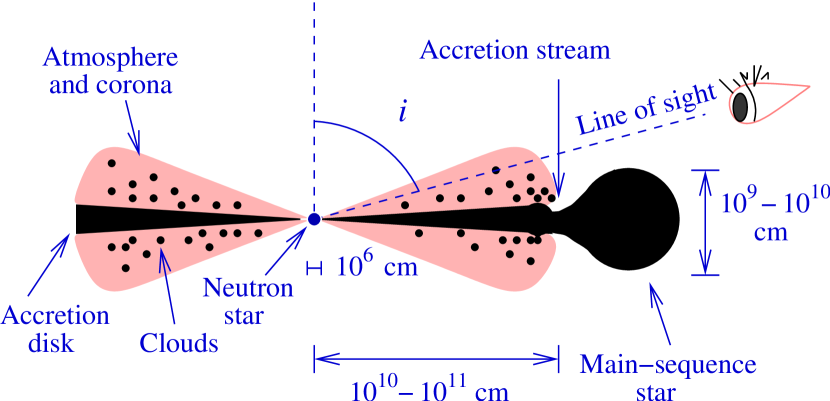
Figure 1: Schematic of a low-mass X-ray binary (LMXB) system with a neutron star primary. Cross section view. The inclination angle $i$ is defined.

The X-ray line emission arises presumably as the result of irradiation of the disk by the X-ray continuum, producing an extended source of reprocessed emission. Evidence of X-ray emission from extended regions in LMXBs comes from the spectral variations during ingress and egress phases of eclipses, and during rapid intensity fluctuations known as dips. Most dips, which are observed to precede eclipses, are thought to result from variable obscuration and attenuation of the primary continuum by material near the outer disk edge, which has been thickened due to impact of the accretion stream with the disk (White & Swank, 1982; Frank, King, & Lasota, 1987). Dips that are uncorrelated with orbital phase can be produced by orbiting clouds crossing the line of sight, as shown in Figure 1. A cloud larger than $\sim 10^{6}$ cm can obscure the X-rays from the neutron star. Hard X-ray emission, presumably originating in the ADC, and representing a few percent of the non-eclipse flux, remains visible during mid-eclipse in several LMXBs, implying that the ADC is larger than the secondary star (White & Holt, 1982; McClintock, London, Bond & Grauer, 1982). LMXB spectra during eclipses or dips may harden or soften, i.e. the proportion between hard ($\sim 3$–10 keV) and soft ($\sim 1$–3 keV) X-rays changes. Most sources harden during dips (Parmar, White, Giommi & Gottwald, 1986), consistent with photoelectric absorption, but there are exceptions like the softening of 4U1624-49 (Church & Balucinska-Church, 1995), and an unchanging X1755-33 (White et al., 1984; Church & Balucinska-Church, 1993). Sources such as EXO0748-67, X1916-05, and X1254-69 show evidence for an unabsorbed spectral component during dips (Parmar, White, Giommi & Gottwald, 1986; Church et al., 1997), revealing an extended source of X-rays which is larger than the ADC. These soft X-rays are likely radiation reprocessed in the accretion disk. Dip ingress/egress times indicate ADC sizes in the $10^{9}$ to $5\times 10^{10}$ cm range, a factor of a few smaller than the accretion disk sizes calculated from typical orbital parameters (Church, 2001). A soft X-ray emission component distinct from the hard X-ray continuum has also been interpreted as being due to the effects of absorption edges or line emission in some LMXBs (Parmar et al., 2000; Church et al., 1998). The unequivocal identification of the accretion disk X-ray emission, requires both an energy resolution that is higher than CCD detectors, and high throughput, plus a quantitative theoretical prediction of the X-ray emission from the disk. We discuss the recently observed high resolution spectra in section 8.1.

2.2 Radiatively heated accretion disks

2.2.1 Radial structure

In LMXBs roughly half of the gravitational potential energy is released in the vicinity of the compact object (i.e., in a boundary layer near the neutron star surface). The disk is exposed to this radiation, and it will be heated by it. Radiative heating can exceed internal viscous heating in the outer region of the disk. The temperature structure of the disk can thus be controlled by the X-ray field photoionizing the gas, suppressing convection, and increasing the scale height of the disk.

Assuming that all the viscous heating and radiative heating from illumination by the central source is radiated locally as a blackbody (as in the SS73 model), Vrtilek et al. (1990) calculated the temperature for a geometrically thin disk, with $r\gg R_{1}$, where $R_{1}$ is the radius of the compact X-ray source:

$$\sigma T_{\rm phot}^{4}\simeq\frac{3GM_{1}\dot{M}}{8\pi r^{3}}+\frac{(1-\eta)L_{\rm x}\sin\theta(r)}{4\pi r^{2}},$$ (1)

where $T_{\rm phot}$ is the photospheric temperature, $M_{1}$ is the mass of the compact X-ray source, $G$ is the gravitational constant, $\sigma$ the Stephan-Boltzmann constant, $\theta$ is the grazing angle of the incident X-ray flux with respect to the disk surface, and $\eta$ is the X-ray albedo such that $(1-\eta)$ is the fraction of X-rays absorbed at the photosphere. The albedo has been derived from optical observations (de Jong, van Paradijs, & Augusteijn, 1996). The first term on the right-hand side of equation (1) is the energy dissipated within the SS73 disk, and the second term is the radiative heating. The radiative heating term will dominate where

$$r>2.3\times 10^{8}~{}\biggl{(}\frac{M_{1}}{M_{\sun}}\biggr{)}~{}\biggl{(}\frac{1-\eta}{0.1}\biggr{)}^{-1}~{}\biggl{(}\frac{\sin\theta}{0.1}\biggr{)}^{-1}~{}\biggl{(}\frac{\epsilon_{\rm x}}{0.1}\biggr{)}^{-1}~{}\rm cm,$$ (2)

where the X-ray luminosity is written in terms of an X-ray accretion efficiency $\epsilon_{\rm x}$, according to $L_{\rm x}=\epsilon_{\rm x}\dot{M}c^{2}$. For example, accretion onto a neutron star results in roughly 1/2 of the gravitational potential energy being converted into X-rays, or $\epsilon_{\rm x}=GM_{1}/2c^{2}R_{1}$. The disk, therefore, is radially divided in two regions: an inner region dominated by internal dissipation, and an outer region dominated by external illumination. External radiation will dominate the disk atmosphere energetics for the outer two or three decades in radii, and the local dissipation and magnetic flare heating, if any, will be ignored there (see also section 8.3).

2.2.2 Vertical Structure

The radial dependence of the disk temperature in equation (1) relies on averaging physical quantities such as the dissipation parameter $\alpha$ in the direction perpendicular to the disk plane, which is valid for regions in the disk that are optically thick. However, as we will show in this article, the radiative recombination spectrum is very sensitive to the radial and the vertical ionization structure, including regions with an optical depth $\tau\lesssim 1$.

To obtain a high resolution spectrum of an accretion disk, and in particular one for which the outer (or upper) layers are X-ray photoionized, several authors have calculated the vertical structure by solving the radiation transfer equations, assuming hydrostatic equilibrium. Models have been applied to AGN and LMXBs in the high-$L_{\rm x}$ state, since in the low-state radiatively inefficient accretion ensues, which is described by a separate family of models (Hawley & Balbus (2002) and references therein). In radiatively efficient accretion disks, the radiative transfer is typically simplified by using an on-the spot approximation and the escape probability formalism. Due to photoelectric absorption and Compton scattering, the ionization structure of the disk is stratified, and it is approximated by a set of zones, each with a single ionization parameter. The ionization structure of the disk can be solved by using photoionization codes such as CLOUDY (Ferland et al., 1998) and XSTAR (Kallman & McCray, 1982), which calculate the ionization and thermal equilibrium state of the gas at each zone.

Ko & Kallman (1991, 1994) calculated the vertical structure of an illuminated accretion disk and obtained the recombination X-ray spectrum for individual rings on the disk. Raymond (1993) utilized the temperatures in equation (1) and calculated the vertical structure and the UV spectrum from the entire disk. Both assumed parameters for LMXBs, and gas pressure-dominated disks. Later models of photoionized accretion disks focused primarily on calculating the Fe K$\alpha$ fluorescence emission from AGN disks.

Różańska & Czerny (1996) and Różańska, Czerny, Życki & Pojmański (1999) modeled semi-analytically the stratified, photoionized transition region between the corona and the disk in AGN. They found that their approximations, which included on-the-spot absorption, matched more accurate radiation transfer codes for optical depths $\lesssim 10$. They also discussed the existence of a two-phase medium, stopping short, however, of calculating an X-ray spectrum. Nayakshin, Kazanas & Kallman (2000) modeled a radiation-pressure dominated disk and showed that the vertical structure of the disk implied significant differences in the Fe K fluorescence line spectrum compared to that predicted by constant-density disk models (Ross & Fabian, 1993; Matt, Fabian & Ross, 1993; Zycki, Krolik, Zdziarski & Kallman, 1994). In addition, Nayakshin, Kazanas & Kallman (2000) also found that the gas was thermally unstable at certain ionization parameters, which created an ambiguity in choosing solutions and a sharp transition in temperature in the disk. This instability is discussed in section 4. Ballantyne, Ross, & Fabian (2001) calculated the vertical structure of disk ring as a function of radius, accretion rate, the angle of incidence of radiation, the photon index, and the black hole mass, albeit using a diffusion approximation. Różańska, Dumont, Czerny, & Collin (2002) calculated the hydrostatic disk structure including Compton scattering and line transfer without assuming the escape probability approximation. Różańska, Dumont, Czerny, & Collin (2002) also calculated the structure of the optically thick part of the disk, by use of the diffusion approximation and the local $\alpha$-prescription (Eq. [12]). All of the above models calculate the disk structure for one radius at a time.

Li, Gu, & Kahn (2001) found the static solution that resolves the thermal instability in the gas by considering the effect of conduction, and they computed the X-ray recombination and resonance line scattering spectrum for the conduction transition region that forms between stable solutions in the disk. With this procedure, the unphysical, sharp transition between stable phases was eliminated. Li et al. considered ionizing continua typical of AGN, which can yield stable solutions with three different temperatures for a given pressure ionization parameter $\Xi$ (defined in section 3.3). Up to three distinct transition layers can form. The reflection and recombination spectrum of the transition regions in the 0.5–1.5 keV range was computed by considering the vertical structure of an isobaric, optically thin region. They found that resonant scattering can be important within the transition region, depending on the local gravity and luminosity, which yields a line spectrum which is different from that of pure recombination emission.

The vertical structure of an optically thick accretion disk can be obtained using the diffusion approximation, which assumes that the photon mean free path $\lambda$ is much smaller than the scale of temperature and density gradients $T/\nabla T$ and $\rho/\nabla\rho$, respectively. Adding convective heat transfer by introducing an adiabatic temperature gradient, Meyer & Meyer-Hofmeister (1982) have calculated the vertical structure of an isolated accretion disk which is dominated by convection zones. Such techniques are used in the standard stellar structure equations. X-ray illumination from the central compact object suppresses convection, reduces the thermal gradients in the disk, and has a stabilization effect in the outer radii; but if X-ray illumination is combined with the diffusion approximation, it also produces a convex disk that self-shadows the outer disk regions. This contradicts the observed spectra, which show evidence of reprocessing from the outer disk (Dubus et al., 1999). A semi-analytical model using a variable $\alpha$-viscosity prescription was used to model AGN disks and to investigate its effects on the Lyman edge absorption and emission (Różańska, Czerny, Życki & Pojmański, 1999).

The failure of the diffusion-equation models to reproduce a concave disk that can efficiently reprocess the central X-rays may indicate that important effects were neglected. First, the effect of the disk atmosphere and corona was ignored. Second, turbulent heat transfer may produce a vertical disk structure that is nearly isothermal. The strong turbulence occurring at the scale of the disk thickness in magneto-hydrodynamic (MHD) models supports this hypothesis (Miller & Stone, 2000). A reliable calculation of the turbulent heat transfer in an accretion disk is needed. Therefore, we prefer to use the Vrtilek et al. (1990) vertically-isothermal disk for the optically thick region.

The diffusion approximation is inadequate when calculating high resolution spectra since line radiation must originate in a region where the photon mean-free-path $\lambda$ exceeds the scale of the temperature gradient, i.e. $\lambda\gtrsim T/\nabla T$. Thus, just as for stellar atmospheres (Mihalas, 1978), an explicit radiation transfer calculation without assumption of local thermodynamic equilibrium is needed. The modeling of photoionization heating, recombination cooling, and X-ray opacities is then required in the atmosphere.

3 Model atmosphere

We consider a LMXB with a $M_{*}=1.4$ $M_{\sun}$ primary radiating an Eddington luminosity ($L_{\rm x}=10^{38.3}$ erg s^-1) bremsstrahlung continuum, with $T=8$ keV. A set of fiducial system parameters for a bright LMXB is used, so application to a particular source will require using the observed X-ray continuum to improve accuracy. The maximum radius of the centrally-illuminated disk is $10^{11}$ cm, so the orbital period $\sim 1$ day. The minimum radius is $10^{8.5}$ cm, below which the omitted effect of radiation pressure, in large part, determines the disk structure.

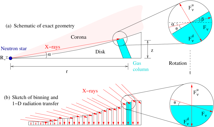
Figure 2: Side view schematic of an illuminated accretion disk and the model geometry, assuming an extended corona above the disk. To compute the ionization structure of the disk, the disk geometry (a), can be approximated by a series of gas columns which are illuminated from the top (b).

The vertical structure of the disk atmosphere for each annulus in the array, is obtained by integrating the hydrostatic balance and 1-D radiation transfer equations for a slab geometry (Fig. 2):

$$\frac{\partial P}{\partial z}=-\frac{GM_{*}\rho z}{r^{3}}$$ (3)

$$\frac{\partial F_{\nu}}{\partial z}=-\frac{\kappa_{\nu}F_{\nu}}{\sin\theta}$$ (4)

$$\frac{\partial F_{\nu}^{\rm d}}{\partial z}=-\kappa_{\nu}F_{\nu}^{\rm d}$$ (5)

while satisfying local thermal equilibrium (see also eq. [3.4]):

$$\Lambda(P,\rho,F_{\nu})=0$$ (6)

and ionization balance (see also eq. [13]):

$${\rm ion\ formation\ rate}={\rm ion\ destruction\ rate}$$ (7)

where $P$ is the total pressure, $\rho$ is the mass density, $F_{\nu}$ is the net flux of incident radiation (which is the intensity integrated over all solid angles in erg cm^-2 s^-1 Hz^-1), $F_{\nu}^{\rm d}$ is the reprocessed net flux propagating down towards the disk midplane, $z$ the vertical distance from the midplane, $G$ the gravitational constant, $\theta$ the grazing angle of the radiation on the disk, $r$ the radius, $\nu$ is the frequency, and $\kappa_{\nu}$ is the local absorption coefficient. The rays corresponding to $F_{\nu}$ and $F_{\nu}^{\rm d}$ are defined in Figure 3. Hydrostatic equilibrium is satisfied to a $\lesssim 1$% accuracy and thermal balance to $\lesssim 0.01$%.

For the structure calculation only, 100 logarithmically spaced energy bins, in the range $1$ eV $<h\nu<1000$ keV, were used for $F_{\nu}$ and $F_{\nu}^{\rm d}$. The grid is coarse, and yet sufficiently broad to accomodate a hard X-ray tail in future models. The reprocessed radiation propagating upwards, $F_{\nu}^{\rm u}$, is omitted to accelerate the computation. This is a good approximation since the radiative heating is dominated by the direct flux $F_{\nu}$. The reprocessed flux $F_{\nu}^{\rm u}$ is calculated a posteriori by a high resolution spectral model (section 5). The difference between cooling and heating, $\Lambda$, includes Compton scattering, bremsstrahlung cooling, photoionization heating, collisional line cooling, and recombination line cooling (section 3.4). Cosmic abundances (Allen, 1973) are assumed. The code from Raymond (1993) computes the net heating and ionization equilibrium, models Compton scattering in one dimension, and calculates line scattering using escape probabilities. A new disk structure calculation simultaneously integrates equations (3)–(5) by the Runge-Kutta method, using an adaptive step-size control routine with error estimation, and equation (6) is solved by a globally convergent Newton’s method (Press, 1994). At the ADC height $z_{\rm cor}$, the equilibrium $T$ is close to the Compton temperature $T_{\rm compton}$, from which we begin to integrate downward until $T<T_{\rm phot}(r)$. The optically thick part of the disk, with temperature $T_{\rm phot}$, is assumed to be vertically isothermal (Vrtilek et al., 1990). To get $T_{\rm phot}$, the viscous energy and the illumination energy are assumed to be locally (re)radiated with a blackbody spectrum. Thus, for $z_{\rm phot}\ll r$ and $R_{*}\ll r$, equation (1) can be used with $M_{1}\equiv M_{*}$. The height at which the integration ends is defined as the photosphere height $z_{\rm phot}$. Thus, we assume that viscous dissipation dominates heating for $z<z_{\rm phot}$ (Fig. 3).

The boundary conditions, shown schematically in Figure 3, are set at the ADC to $P(z_{\rm cor})=\rho_{\rm cor}kT_{\rm compton}/\mu m_{p}$, $\int F_{\nu}(z_{\rm cor})d\nu=L_{x}/4\pi r^{2}$, and $F_{\nu}^{\rm d}(z_{\rm cor})=0$, where $k$ is the Boltzmann constant, and $\mu$ is the average atomic weight of baryons in units of the proton mass $m_{p}$. The boundary conditions at the photospheric height ($=z_{\rm phot}$) for $F_{\nu}$ and $F_{\nu}^{\rm d}$ are set free, and the shooting method (Press, 1994) is used with shooting parameter $\rho_{\rm cor}$, which is adjusted until $P(z_{\rm phot})=\rho_{\rm phot}kT_{\rm phot}/\mu m_{p}$ is satisfied at the photosphere. Note $\rho_{\rm phot}$ is the viscosity-dependent density calculated for an X-ray illuminated SS73 disk.

The shooting method consists of guessing the value of the coronal density which matches the desired pressure at the bottom of the gas column. The boundary conditions define $P_{\rm cor}$ once $\rho_{\rm cor}$ is chosen. Equations (3)–(7) are simultaneously solved during the integration. The temperature drops as the integration proceeds downward through the atmosphere. When $T$ reaches a value below $T_{\rm phot}$, the pressure at that point is compared to the expected pressure of the isothermal disk at that height. If it does not match to better than $\sim$1 %, the integration is repeated with a new estimate of the coronal density. While it is not clear that photoionization will cease to be important for temperatures less than $T_{\rm phot}$, such zones emit negligible X-ray fluxes if $r\gtrsim 10^{9}$ cm. Our new structure calculation also includes the effects of physical instabilities (section 4), and it removes the numerical instabilities obtained by Raymond (1993).

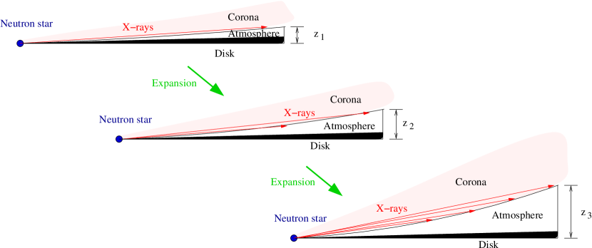
Figure 4: Schematic of the feedback between radiative heating and disk geometry. The heated atmosphere expands and collects more radiation, reaching equilibrium at $\sim 10$ times its initial volume.

A novel and important feature of this model is that the incident radiation is allowed to modify the disk atmosphere geometry, such that the heating and expansion of the atmosphere resulting from illumination are used to calculate the height profile of the atmosphere as a function of radius. This feedback between the radiative heating and the atmospheric structure is depicted in Figure 4. The atmospheric height is used to derive the input grazing angle of the radiation for the next model iteration. This contrasts with calculating the grazing angle using the pressure scale height of the optically thick disk (Vrtilek et al., 1990), which is in general much smaller than the photoionized atmosphere, and which underestimates the grazing angle and the line intensities by an order of magnitude. To get $T_{\rm phot}$ self-consistently from equation (1), the equation

$$\theta(r) \simeq \beta-\alpha+\arctan\biggl{(}\frac{R_{*}}{r}\biggr{)}$$ (8)

$$= \arctan\biggl{(}\frac{dz_{\rm atm}}{dr}\biggr{)}-\arctan\biggl{(}\frac{z_{\rm atm}}{r}\biggr{)}+$$

$$\arctan\biggl{(}\frac{R_{*}}{r}\biggr{)}$$

is needed, where $z_{\rm atm}(r)$ is defined as the height where the frequency-integrated grazing flux $\int F_{\nu}(z_{\rm atm})~{}d\nu$ is attenuated by $e^{-1}$, and $\alpha,\beta$ are defined in Figure 2. The $\arctan(R_{*}/r)$ term is neglected, which is valid for $r\gtrsim 10^{8.5}$ cm. As discussed above, $\theta(r)$ is calculated iteratively from equation (8). After an initial guess for $z_{\rm atm}(r)$, it is re-calculated from the newly obtained disk structure. A power-law fit to $z_{\rm atm}(r)$ works well to obtain $\theta(r)$. This iteration is performed with a limited number of radial bins (5), to save computation time. The iteration is stopped after $\theta(r)$ and $T_{\rm phot}$ converge to $\lesssim 10$ %. After convergence, the number of logarithmically spaced radial bins is increased to 26. The process of convergence does not depend on the initial choice of $\theta(r)$, and it is shown in Figure 5. However, convergence does depend on the choice of $z_{\rm atm}$, which is a free parameter in the model. Since $z_{\rm atm}$ is not physically determined, it must be defined ad hoc, but it is bound by $z_{\rm atm}>z_{\rm phot}$. For $z\lesssim z_{\rm phot}$, the illumination $F_{\nu}\rightarrow 0$, and the disk blackbody flux $F_{\rm bb}(T_{\rm phot})$ takes over. To test how sensitive is the result to the definition of $z_{\rm atm}$, we calculate $\theta(r)$ taking $z_{\rm atm}=z_{\rm phot}$, and we use this to estimate the systematic errors of the 1-D radiation transfer calculation.

3.1 The Choice of Assumptions

The validity of the assumptions is reviewed, both for the the model presented here and for some of the accretion disk models in the astrophysical literature.

For modeling X-ray line emission from the disk atmosphere, the commonly used assumptions of $LTE$ and the diffusion approximation will not hold. In addition, assuming a constant density in the vertical direction will be inadequate, since the hydrostatic equilibration time is small or comparable to other relevant timescales, and the line emission is highly sensitive to the vertical ionization structure. The recombination emission is especially sensitive to this structure, since each ion emits clearly resolvable line energies. Also, fluorescence emission can be reprocessed by a Compton-thick, fully ionized gas above it (Nayakshin, Kazanas & Kallman, 2000).

Thermal equilibrium and ionization equilibrium are reasonable assumptions in a time averaged sense. Hydrostatic equilibrium is also assumed, to avoid explicit computation of the plasma dynamics with radiative transfer. Deviations from hydrostatic equilibrium are smoothed in the timescale

$$t_{\rm hydro}=z_{\rm atm}/c_{\rm s}\sim 2.7\biggl{(}\frac{z_{\rm atm}}{10^{7}~{}{\rm cm}}\biggr{)}T_{5}^{-1/2}\ \ \rm sec$$ (9)

where $c_{\rm s}$ is the sound speed. Material from the disk moves radially within the viscous timescale $t_{\rm visc}\sim r^{2}/(\alpha z_{\rm atm}c_{\rm s})>t_{\rm hydro}$ (Frank, King & Raine, 1992), so the gas can reach hydrostatic equilibrium before it flows inward (i.e, the radial accretion velocity is always subsonic). However, the Keplerian orbital velocity $v_{\rm k}\gg c_{\rm s}$ is highly supersonic. If the gas flow in the corotating frame of the gas is also supersonic, then shocks would collisionally ionize and heat the gas. In such a case, the observed spectrum of the disk would significantly deviate from a photoionized gas in ionization and thermal equilibrium. The thermalization and ionization equilibrium timescale of the atmosphere is driven by the recombination timescale

$$t_{\rm th}=t_{\rm rec}\sim 0.3\biggl{(}\frac{T_{5}^{1/2}}{n_{14}Z^{2}}\biggr{)}\ \ \rm sec$$ (10)

which can be derived from equation (A3), and where $T_{5}$ is the temperature in units of $10^{5}$ K, $n_{14}$ is the density in units of $10^{14}$ cm^-3, and $Z$ is the atomic number (Reynolds & Fabian, 1995). The photoionization timescale is shorter than $t_{\rm rec}$ where the gas is fully stripped; otherwise both timescales are comparable for the relevant ions having similar abundances. The Coulomb collision relaxation timescale between electrons and ions $t_{\rm ep}$ is slower than between identical particles, and is (Spitzer, 1962)

$$t_{\rm ep}\simeq 3\times 10^{-6}\frac{T_{5}^{3/2}}{n_{14}}\ \ {\rm sec}.$$ (11)

Electron-electron relaxation is $\sim m_{\rm p}/m_{\rm e}$ times faster, and proton-proton relaxation is $\sim\sqrt{m_{\rm p}/m_{\rm e}}$ times faster. For the hot corona at the outer disk at $T\sim 10^{7}$ K and $n_{\rm e}\sim 10^{11}$ cm^-3 (from the coronal structure in section 6), the relaxation timescale is $t_{\rm ep}\sim 3$ sec. The fully ionized gas in the corona, which is near the Compton temperature, has a thermal timescale of $t_{\rm th}=t_{\rm compton}=10r_{10}^{2}L_{38}^{-1}$ sec, where $r_{10}$ is the disk radius in units of $10^{10}$ cm, and $L_{38}$ is the X-ray luminosity in units of $10^{38}$ ergs^-1 (Reynolds & Fabian, 1995). Thus, thermalization in the disk atmosphere and corona is driven by the ionization timescales, since the Coulomb relaxation times are comparatively fast due to the large density. Thermal and ionization equilibrium occur faster than hydrostatic equilibrium, for length scales $z_{\rm atm}\gtrsim 10^{6}$ cm. If $t_{\rm th}<t_{\rm hydro}$, luminosity fluctuations with timescales $t_{\rm flux}$ such that $t_{\rm th}<t_{\rm flux}<t_{\rm hydro}$ will take the gas outside hydrostatic equilibrium, but not out of thermal equilibrium. Integrated spectral observations on timescales $t\gg t_{\rm flux}$ cannot observe this effect.

The radiation transfer is complex, and the assumptions used to simplify calculations could be problematic. In particular, by dividing the disk atmosphere into annular zones with a given vertical gas column, our 1-D radiation transfer calculation assumes that 1) the primary continuum is not absorbed before reaching the top of the column, 2) the radiation in the column propagates from top to bottom at a given grazing angle, and 3) there is no significant radiative coupling from one disk annulus to another, which is used to justify the slab approximation. The above assumptions are inadequate if the column height is comparable to the disk radius, or if the photon mean free path in the gas column is many times the local radius. Thus, future 2-D calculations will result in better bookkeeping of photons, a more accurate structure, and a more reliable X-ray line spectrum.

The correct calculation of line transfer in the gas is also a concern, since the disk atmosphere is optically thick in the lines (section 6). Line transfer is complicated by the Keplerian velocity shear, which has to be taken into account for a given viewing angle (Murray & Chiang, 1997). The escape-probability approximation used to calculate line transfer in the disk may also be inadequate because of the large optical depths.

Our calculations show that the proper treatment of a thermal instability (Field, 1965; Krolik, McKee & Tarter, 1981) and conduction affect the spectrum significantly (Zeldovich & Pikelner, 1969; Li, Gu, & Kahn, 2001) (section 4). A two-phase gas could form, with clouds of an unknown size distribution and with undetermined dynamics of evaporation and condensation (Begelman & McKee, 1990), with each phase having distinct ionization parameter and opacity. The instability is sensitive to 1) the metal abundances, 2) the continuum shape (Hess, Kahn, & Paerels, 1997), and 3) the atomic kinetics (Savin et al., 1999).

The local viscous energy dissipation rate per unit volume in the disk atmosphere may be included in equation (6) with the form (Czerny & King, 1989, SS73)

$$Q_{\rm visc}=\frac{3}{2}\Omega\alpha P$$ (12)

where $\Omega$ is the Keplerian angular velocity, $\alpha$ is the viscosity parameter, and $P$ is the local pressure. Equation (12) is an extension of the $\alpha$-disk model (where the viscous dissipation is vertically averaged), and it assumes the local validity of the $\alpha$ prescription, which is untested. Fortunately, our numerical modeling indicates that the viscosity term is negligible in most regions of the disk atmosphere except for the inner disk and $\alpha\sim 1$ (in particular, near the Compton-temperature corona). This viscosity term enhances a thermal instability between $10^{6}$ and $10^{7}$ K. Vertically stratified MHD models (Miller & Stone, 2000), although inconclusive, owing to the uncertain effect of boundary conditions, show that the viscous dissipation drops rapidly at $\gtrsim 2$ pressure scale heights away from the disk midplane, providing evidence against equation (12). Since the disk atmosphere is always a few scale heights above the midplane, we choose not to include equation (12) in our models. Equation (12) has been applied in the optically thick regions of the disk by Dubus et al. (1999) and in the disk atmosphere by Różańska & Czerny (1996). Other forms for the local dissipation that reduce to the $\alpha$-disk have been used (Meyer & Meyer-Hofmeister, 1982).

3.2 Ionization balance

In steady state the equation of ionization balance for each ion $Z^{+i}$ is

$$\frac{\partial n_{z,i}}{\partial t} = n_{z,i+1}n_{\rm e}\alpha_{z,i+1}+n_{z,i-1}(\beta_{z,i-1}+n_{\rm e}C_{z,i-1})$$ (13)

$$-n_{z,i}(\beta_{z,i}+n_{\rm e}\alpha_{z,i}+n_{\rm e}C_{z,i})$$

$$+n_{z,i-2}\beta_{z,i-2}^{\rm K}B_{z,i-1}=0,$$

where $\beta_{z,i}$ is the photoionization rate (s^-1) of $Z^{+i}$, $C_{z,i}$ is the collisional ionization rate coefficient ($\rm{cm^{3}~{}s^{-1}}$) of $Z^{+i}$, $\alpha_{z,i+1}$ is the recombination rate coefficient ($\rm{cm^{3}~{}s^{-1}}$) of ion $Z^{+(i+1)}$, and so on. The code also includes K-shell photoionization followed by Auger ionization in the last term of equation (13). The Auger branching fraction is $B_{z,i-1}=1-Y_{z,i-1}$, where $Y_{z,i-1}$ is the fluorescence yield. Multiple Auger decays are ignored in equation (13). The terms with $\alpha_{z,i+1}$ and $\alpha_{z,i}$ account for all two-body recombination processes. The coefficients $C_{z,i}$ and $\alpha_{z,i}$ depend on the electron temperature $T$ for any ion $Z^{+i}$. Given the photoionization cross-section $\sigma_{PE,z,i}$ and ionization threshold energy $\chi_{z,i}$ of the ion $Z^{+i}$, the photoionization rate for a point source of ionizing continuum is

$$\beta_{z,i}=\frac{L_{\rm x}}{r^{2}}~{}\int_{\chi_{z,i}}^{\infty}dE~{}\frac{S_{E}(E)}{4\pi E}~{}\sigma_{PE,z,i}(E),$$ (14)

where $S_{E}$ is the spectral shape function, normalized on a suitable energy interval. For the accretion disk atmospheres orbiting neutron stars, which are of interest here, collisional ionization rates are negligible compared to photoionization rates.

3.3 The ionization parameter

Let $\xi=L_{\rm x}/n_{\rm p}r^{2}$ (in erg s^-1 cm) be the ionization parameter, where $n_{\rm p}$ is the proton number density (Tarter, Tucker & Salpeter, 1969). The ionization parameter $\xi$ is factored out of equation (14), and together with the spectral shape function $S_{E}$, it defines uniquely the charge state distribution in an optically thin photoionized gas (eq. [13] does not include three-body recombination, which is important at $n_{e}\gtrsim 10^{16}$ cm^-3).

Another, dimensionless ionization parameter is constructed with the radiation pressure $P_{rad}$ and the proton gas pressure $P_{gas}$ (Krolik, McKee & Tarter, 1981). This ionization parameter, $\Xi$, is defined as $\Xi\equiv P_{rad}/P_{gas}$, where $P_{rad}=\int F_{\nu}d\nu/c$. Note $\Xi=\xi/4\pi ckT$. The new parameter $\Xi$ is useful when the local pressure can be defined. For an optically thin gas, an isobar has constant $\Xi$.

3.4 Thermal Equilibrium

We review the terms in the thermal equilibrium equation, which we solve with the Raymond (1993) photoionized plasma code. Thermal equilibrium is enforced at each zone in the disk atmosphere. The explicit form of the thermal equilibrium condition, equation (6), is

$${\rm Compton\ net\ heating}+{\rm photoionization\ heating}=$$

$${\rm bremsstrahlung\ cooling}+{\rm recombination\ cooling}$$

$$+{\rm collisional\ cooling},$$ (15)

which corresponds to (Halpern & Grindlay, 1980)

$$\int F_{\nu}\biggl{(}n_{\rm e}\Gamma^{{\rm com}}_{\nu}+\sum_{z,i}n_{z,i}\Gamma_{\nu,z,i}^{{\rm phot}}\biggr{)}d\nu=$$

$$n_{\rm e}\sum_{z,i}n_{z,i}(\Lambda_{z,i}^{{\rm brem}}+\Lambda_{z,i}^{{\rm rec}}+\Lambda_{z,i}^{{\rm col}})$$ (16)

in units of erg s^-1 cm^-3, where the rates for each process and other dependencies are included in the group of rate coefficients $(\Gamma^{{\rm com}}_{\nu},\Gamma_{\nu,z,i}^{{\rm phot}},\Lambda_{z}^{{\rm brem}},\Lambda_{z,i}^{{\rm rec}},\Lambda_{z,i}^{{\rm col}}$), $n_{\rm e}$ is the electron number density, $n_{z,i}$ is the $Z^{+i}$ ion density, and the sums are performed over all abundant ions. The radiative heating is directly proportional the net flux $F_{\nu}$ (in units of erg s^-1 cm^-2 Hz^-1), and the density. Cooling processes, which originate from electron-ion interactions, are proportional to the square of the density and are in general dependent on the electron temperature $T$. The coefficients in equation (3.4) can be obtained from Halpern & Grindlay (1980), and some, such as the recombination coefficients, are very dependent on the available atomic data. A list of the data used for the coefficients in the model, and a list of the processes and transitions included in the calculations can be found in Raymond (1993). Recombination cooling includes both radiative recombination and dielectronic recombination. Collisional cooling includes cooling due to line emission and collisional ionization. Photon trapping and subsequent collisional de-excitation reduces the cooling rate compared to the optically thin case, but this affects the UV lines more than the X-ray lines because the resonant scattering opacity is larger in the UV.

The ions of H, He, C, N, O, Ne, Mg, Si, S, Ar, Ca, and Fe are included in the thermal equilibrium equation (3.4), and the ionization balance equation (13).

For a fully ionized gas, such as the hot corona above the accretion disk, Compton heating and inverse-Compton cooling dominate equation (3.4). The Compton net heating term may be positive or negative, since the transfer of energy between the photons and the electron gas depends on the electron temperature and the shape of the ionizing spectrum. In such cases, and in the non-relativistic case, the equilibrium temperature is

$$T_{\rm compton}=\frac{h\int\nu F_{\nu}d\nu}{4k\int F_{\nu}d\nu}$$ (17)

where $k$ and $h$ are the Boltzmann and the Planck constants, respectively. The Compton temperature $T_{\rm compton}$ is determined uniquely by the shape of the ionizing continuum. For an 8 keV bremsstrahlung spectrum, $T_{\rm compton}\sim 2\times 10^{7}$ K.

4 Thermal Instability in Photoionized Gases

Irradiated gas is subject to thermal instabilities for temperatures in the $10^{5}$–$10^{7}$ K range (Buff & McCray, 1974; Field, 1969), such that X-ray line emission at those temperatures may be suppressed. The Field (1965) stability criterion, together with plasma equilibrium calculations Davidson & Netzer (1979); Kallman & McCray (1982); Raymond (1993); Ferland et al. (1998), indicate that a photoionized gas becomes thermally unstable when recombination cooling of H- and He-like ions is important. Consequently, the disk atmosphere structure has a thermally unstable region, which modifies the X-ray spectrum.

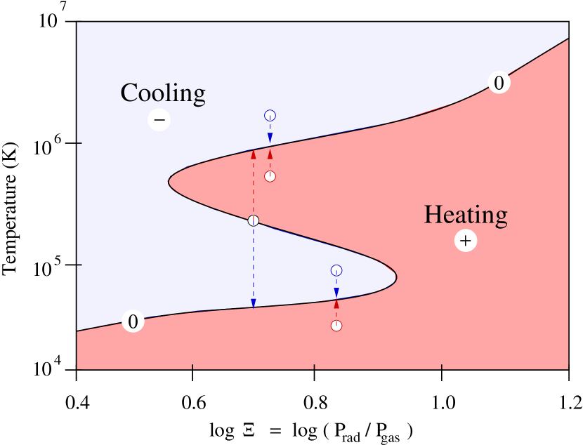
Figure 6: Map of net heating in the gas, in the temperature $T$ vs. ionization parameter $\Xi$ plane. The thermal equilibrium S-curve is labeled with “0”. The dashed arrows depict the thermodynamics of the gas after an isobaric temperature perturbation, starting from points on the S-curve.

To clarify the nature of the thermal instability, consider the calculated net heating (Fig. 6). The gas is externally heated, and the net heating depends on the state variables and ionization of the gas, making this a peculiar system. The thermal balance locus, where the net heating is zero, is denoted as the S-curve and is displayed in Figure 6. The region to the left of the S-curve undergoes net cooling, and the one to the right has net heating.

To test stability, consider small $T$-perturbations starting from the S-curve. A vertical displacement from any point in Figure 6 represents an isobaric perturbation in $T$. From this, we find that the points in the S-curve with positive slope are stable, while those with negative slope are unstable (Field, 1965). This splits the S-curve into three branches. The shape of the S-curve determines which range of $\Xi$ are unstable (section 3.3). At such $\Xi$, thermal balance is achieved by three distinct $T$ on the S-curve, two stable $T$ and one unstable $T$. On the unstable branch, isobaric $T$-perturbations cause a thermal runaway to one of the stable branches.

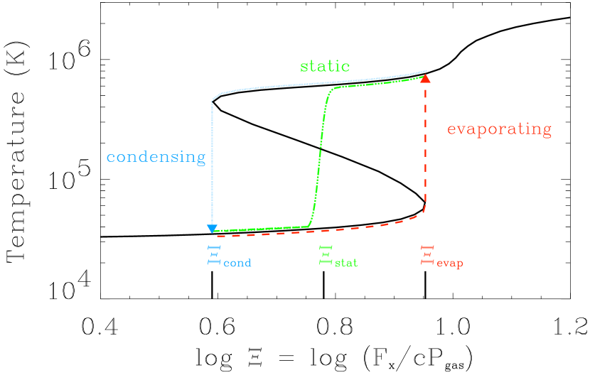
Figure 7: Ionization parameter $\Xi$ vs. temperature assuming an 8 keV bremsstrahlung continuum. The calculated S-curve corresponds to the locus of solutions in thermal balance and ionization equilibrium. The branch of the S-curve with a negative slope is thermally unstable. We over-plot three additional solutions which, due to the addition of a conduction term in the energy equation, avoid the unstable branch. The family of solutions which include conduction produce a small transition region. We model the two extreme cases, the evaporating and condensing disks, which include the lower and upper stable branches of the curve, respectively. A third, static solution, produces a transition at an intermediate $\Xi$. Schematics of the static transition region at $\Xi_{\rm stat}$ and the dynamic transition regions at $\Xi_{\rm cond}$ and $\Xi_{\rm evap}$ are shown. For $\log\Xi>1.2$, $T$ increases up to $T_{\rm compton}\sim 10^{7}$ K (not shown).

The shape of the S-curve depends on the metal abundances and the ionizing spectrum (Hess, Kahn, & Paerels, 1997). The S-curve is subject to uncertainties in the atomic data (Savin et al., 1999), and its shape may vary (albeit not dramatically) from one plasma code to another. Our calculated S-curve for the disk atmosphere is shown in Figure 7.

Most spectral studies of heated accretion disks in LMXBs and AGN have either used unstable solutions, or just selected a subset of the stable solutions. Różańska, Dumont, Czerny, & Collin (2002) chose a monotonic density, which is equivalent to selecting all points on the S-curve. This results in a pressure which oscillates with height and a transition region which is not in hydrostatic equilibrium. Ko & Kallman (1994) and Nayakshin & Kallman (2001) selected the hot branch of solutions, which produce a condensing atmosphere biased towards high-ionization species. Ballantyne, Ross, & Fabian (2001) do not specify how the choice of solutions within the instability was made, but they acknowledge the effects of the instability, which are seen in the sharp temperature transition obtained with their models.

The instability implies a large $\nabla T$ as the gas is forced to move between stable branches, requiring the formation of a transition region whose size may be determined by electron heat conduction, convection, or turbulence, depending on which dominates the heat transfer. For simplicity, calculations of emission from the transition region are omitted in this article. Upon calculation of the Field length $\lambda_{F}$, the lengthscale below which conduction dominates thermal equilibrium (Begelman & McKee, 1990), we estimate that conduction forms a transition layer $\sim 10^{-2}$ times thinner than the size of the X-ray emitting zones. Nevertheless, X-ray line emission from the neglected conduction region may not be negligible in all cases (Li, Gu, & Kahn, 2001). The $\xi$ values present in the transition region are absent in other regions, which may allow the transition region to have observable spectral signatures. Resonant scattering from the transition region may be observable in some situations (Li, Gu, & Kahn, 2001). The importance of the transition region also depends on the shape of the S-curve and on the local gravity.

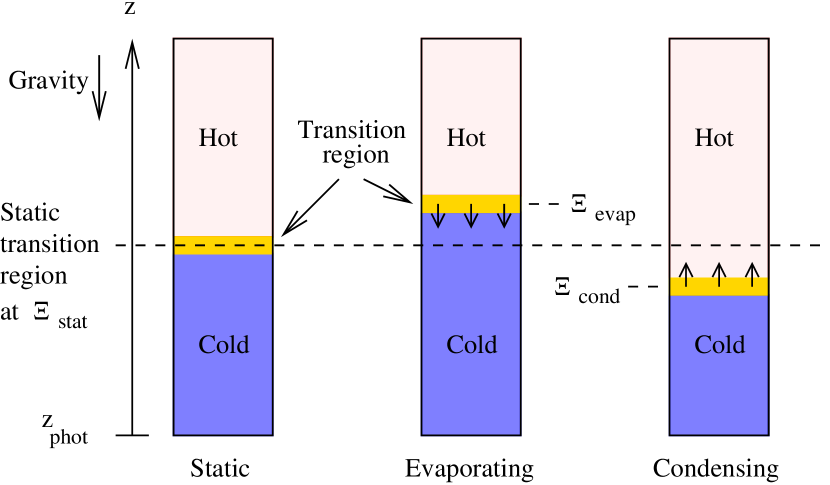
Figure 8: Phase dynamics in a photoionized, stratified gas column. One static and two dynamic cases are shown. A conduction-driven mass flow moves the transition region towards $\Xi_{\rm stat}$ in the condensing and evaporating cases. Due to the boundary conditions at $z_{\rm phot}$, both the pressure and the ionization parameter $\Xi$ are roughly constant at a given height $z$ among the three cases.

Conduction tips the balance of stability at sufficiently small spatial scales. If the gas is not in static equilibrium, conduction can drive phase transitions, and produce dynamic condensing or evaporating fronts. In static equilibrium, conduction quenches the instability and produces a transition layer at $\Xi_{\rm stat}$ (stretching the S-curve in Fig. 7). This transition layer (Zeldovich & Pikelner, 1969) connects the low-$T$ stable branch at $\Xi<\Xi_{\rm stat}$ with the high-$T$ stable branch at $\Xi>\Xi_{\rm stat}$. In the dynamic case, if the transition layer is located away from $\Xi_{\rm stat}$, it will dynamically approach $\Xi_{\rm stat}$ by a conduction driven mass flow, as shown in Figure 8. A transition layer with $\Xi_{\rm stat}<\Xi<\Xi_{\rm evap}$ produces an evaporating front, while a transition layer with $\Xi_{\rm cond}<\Xi<\Xi_{\rm stat}$ produces a condensing front (Zeldovich & Pikelner, 1969; Li, Gu, & Kahn, 2001).

The disk structure for both condensing and evaporating solutions is computed. We assume a steady state, condensing or evaporating mass flow through the transition layer at $\Xi_{\rm cond}$ or $\Xi_{\rm evap}$, respectively. The static equilibrium solution is an intermediate case of the latter extreme cases. A single-valued $T(\Xi)$ is used, since a two-phase solution may be buoyantly unstable, making the denser (colder) gas sink. The evaporating disk corresponds to the low-$T$ branch, while the condensing disk corresponds to the high-$T$ branch (Figure 7). This introduces spectral differences (section 7).

We do not know from first principles whether the disk atmosphere is evaporating, condensing, or static. However, a Compton-heated wind might be expected in the corona for large radii (Begelman, McKee & Shields, 1983). The speed of the conduction mass flow is estimated to be $v_{\rm cond}=2\kappa T/3P_{\rm gas}\lambda_{F}$, by using the characteristic conduction time at the Field length, where $\kappa$ is the Spitzer (1962) conductivity (for a detailed discussion, see McKee & Begelman, 1990). A conduction mass flow speed $v_{\rm cond}=$ 1–2$\times 10^{-2}$ times the local sound speed is obtained. Thus, the phase dynamics will depend on the subsonic ($v\gtrsim v_{\rm cond}$) flow patterns in the disk atmosphere, and these flows will in part determine the evaporation or condensation rates, together with the boundary conditions on mass flow.

If the disk is in a steady state of evaporation or condensation, the implied mass flow can have an effect on the global mass budget, due to mass conservation. Steady state evaporation implies mass loss or a disk wind, while condensation implies a mass gain (Zeldovich & Pikelner, 1969; Li, Gu, & Kahn, 2001).

A thermal instability due to Compton heating and bremsstrahlung cooling can ensue between $10^{6}$ and $10^{7}$ K if the ionizing spectrum extends well above $\sim 10$ keV (Krolik, McKee & Tarter, 1981). For a 8 keV bremsstrahlung spectrum, this additional instability regime is suppressed (Hess, Kahn, & Paerels, 1997). Nevertheless, some LMXBs have harder spectra (White et al., 1995). A double S-curve results from the hard spectra in AGN (Nayakshin & Kallman, 2001), which allows a three-phase gas.

As mentioned above, gas dynamics which are not included in the model can have an impact on the gas phase. The only physical mechanism known to transport the necessary angular momentum for disk accretion involves a magneto-rotational instability (MRI) which drives turbulent flow in the disk (Balbus & Hawley, 1998). These turbulent flows are nearly supersonic in the disk midplane region, where most of the mass is accreted. Enhanced heat transfer rates due to this turbulent flow could quench the thermal instability and affect the disk structure. Turbulent heat transfer rates can be orders of magnitude larger than the saturated conduction heat transfer rate. However, it is not known whether such turbulent motions will also be present in the disk atmosphere, which is several scale heights above the disk midplane and has a density which is orders of magnitude smaller (Section 6). A decline in the viscous $\alpha$ parameter with vertical disk height was obtained with local MHD models, and an enhanced ratio of the magnetic pressure to the gas pressure with increasing height (Miller & Stone, 2000). The MRI also favors the assumption of vertical isothermality in the optically thick disk. In section 8.3, we discuss the effects of magnetic fields in the atmosphere and corona.

5 Spectral modeling

With the disk structure $\rho(r,z)$, $T(r,z)$ and ion abundances $f_{z,i}(r,z)$, the X-ray line emission from the disk atmosphere is calculated using $HULLAC$ data (Klapisch et al., 1977). The code calculates the atomic structure and transition rates of radiative recombination (RR) and the ensuing radiative cascade, which can produce both line photons and radiative recombination continuum (RRC) photons. We include the H-like and He-like ions of C, N, O, Ne, Mg, Si, S, Ar, Ca, and Fe, as well as the Fe L shell ions. Fluorescence emission, which is prominent for high-$Z$ ions such as those of Fe, is omitted in these calculations, as well as resonant scattering, an additional source of line emission. The recombination emissivities, and the opacities in this model, are calculated as described in appendices A and B, respectively.

The spectrum for each of the 26 annuli was added to obtain the disk spectrum. Each annulus consists of a grid of zones in the vertical $\hat{z}$ direction, and $T$, $\rho$ and $f_{z,i+1}$ for each zone are used to calculate the RR and RRC emissivities. The radiation is propagated outwards at inclination angle $i$, including the continuum opacity of all zones above, thus accounting for the optical depth of the atmosphere. Compton scattering of the irradiating continuum is included in the disk structure calculation but it is omitted in the synthetic spectrum. The latter scattering adds a weak continuum component with the spectral shape of the neutron star emission. The spectrum is Doppler broadened by the projected local Keplerian velocity, assuming azimuthal symmetry.

6 Disk structure

Once the atmosphere and corona are accounted for, the disk is thicker than would be expected from the local pressure scale height ($=Z_{\rm P}$) alone. We found $Z_{\rm P}<z_{\rm phot}<z_{\rm atm}$. To quantify the disk geometry, the calculated height of the photosphere and atmosphere, $z_{\rm phot}$ and $z_{\rm atm}$, are both fitted with $z=C(r/1~{}{\rm cm})^{n}$, with fit parameters $C$ and $n$. The fitted parameters are $C_{\rm phot}=(2.4_{-1.9}^{+0.4})\times 10^{-3}$ cm, $n_{\rm phot}=1.14^{+0.06}_{-0.01}$, $C_{\rm atm}=(1.0^{+0.2}_{-0.1})\times 10^{-3}$ cm, $n_{\rm atm}=1.21\pm 0.01$. The above fits imply $z_{\rm phot}\sim 3Z_{\rm P}$ to $4Z_{\rm P}$ (depending on radius) and $z_{\rm atm}\sim(7^{+2}_{-0})Z_{\rm P}$ to $(8^{+2}_{-0})Z_{\rm P}$. We account for statistical errors and estimated systematics. Vrtilek et al. (1990) estimated $n_{\rm atm}=9/7=1.29$, but in spite of the steeper radial dependence, the Vrtilek et al. disk is thinner, and it assumes $z_{\rm atm}=Z_{\rm P}$ for $r>10^{10}$ cm. The disk thickness derived from the optical light curve observations of LMXBs relies on the large fraction of X-rays from the neutron star which are shielded from the companion by the disk. This de facto disk boundary should be taken to be $\sim z_{\rm atm}$, since, by definition, a fraction $1/e$ of the central X-rays are absorbed there. In Figure 9, we compare $Z_{\rm P}$ with $z_{\rm atm}$. We find that previous theoretical studies severely underestimated the size of the disk atmosphere.

The X-ray continuum opacity of the atmosphere is $\tau\ll 1$ for most lines of sight, except for rays originating on the neutron star which are incident at a small grazing angle $\theta(r)$, such that they are nearly parallel to the disk plane. The atmosphere’s ($z>z_{\rm phot}$) maximum photoelectric opacity is always $\tau\ll 1$ in the vertical direction, although $\tau/\sin\theta(r)\gtrsim 1$. Illumination heating dominates at $r\gtrsim$ $10^{10}$ cm (eq. [1]), where only $\int F_{\nu}(z_{\rm phot})d\nu/\int F_{\nu}(z_{\rm cor})d\nu\sim 0.12$ of the incident photons reach $z_{\rm phot}$ directly, while $\int F_{\nu}^{\rm d}(z_{\rm phot})d\nu/(\int F_{\nu}(z_{\rm cor})d\nu\sin\theta)\sim 0.35$ reach $z_{\rm phot}$ after reprocessing in the atmosphere. Thus, the atmospheric albedo is $\sim 0.5$. Both the photosphere and atmosphere contribute significantly to the disk albedo. The total disk albedo deduced by de Jong, van Paradijs, & Augusteijn (1996) from optical observations in LMXBs is $\eta\sim 0.9$. We have found that its high value is partially explained by the atmospheric contribution. Once the latter is taken into account, the photosphere’s albedo becomes $\sim 0.8$, since 0.5+0.5(.8)=0.9, which is closer to physical expectations.

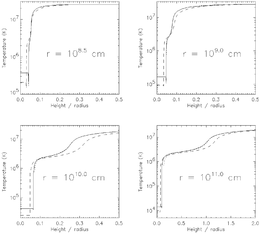
Figure 10: Modeled temperature ($T$) vs. normalized disk height ($z/r$) for various radii. The diagrams can be directly compared to the Raymond (1993) result. Our new model atmosphere is $10\times$ more extended. The chosen stable solutions correspond to a disk under 1) steady evaporation (solid line), 2) steady condensation (dotted line), and 3) steady evaporation at low luminosity $L=0.1L_{\rm Edd}$ (dashed line). The large-scale features of the first two cases are nearly identical.

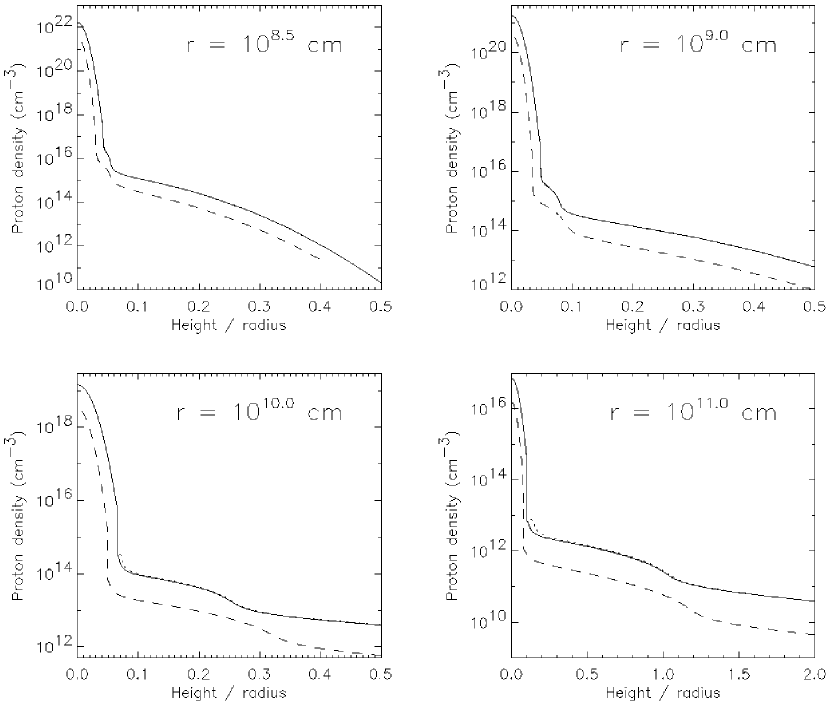
Figure 11: Modeled proton density ($n_{p}$) vs. disk height ($z$) for various radii. Evaporating (solid line), condensing (dotted line), and low-luminosity (dashed line) disk models, as in Fig. 10. The height is normalized to the local radius.

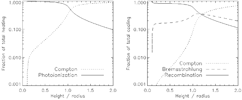
Figure 12: Dominant heating and cooling mechanisms versus the vertical height of the atmosphere, for the disk annulus with $r=10^{11}$ cm. A Compton-heated corona and a recombining atmosphere can be discerned.

At any fixed radius, the vertical disk structure has a marked boundary between the optically thick, colder disk and an optically thin, hotter atmosphere, as shown in Figures 10 and 11. At the largest scales, the vertical structure has two distinct zones: a hot corona, in which Compton heating and cooling dominates, and an atmosphere or warm corona, where photoionization heating and recombination cooling are most important. Three regions are discernible in Figure 12, which shows the vertical structure of the outer radius of the disk (other radii show a similar pattern, aside from changes in scale).

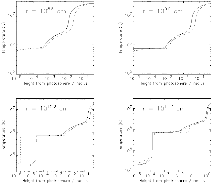
Figure 13: Modeled temperature ($T$) vs. disk atmosphere height above the photosphere ($z_{\rm atm}-z_{\rm phot}$) for various radii. Evaporating (solid line), condensing (dotted line), and low-luminosity (dashed line) disk models. The height is normalized to the local radius.

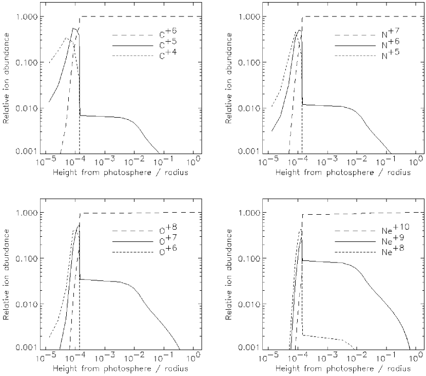
Figure 15: Vertical distribution of low-$Z$ ions for the evaporating disk model. Low charge states are omitted for clarity. The relative ion abundances are plotted against $(z_{\rm atm}-z_{\rm phot})/r$, the vertical height of the atmosphere, for the disk annulus with $r=10^{11}$ cm, which dominates line emission.

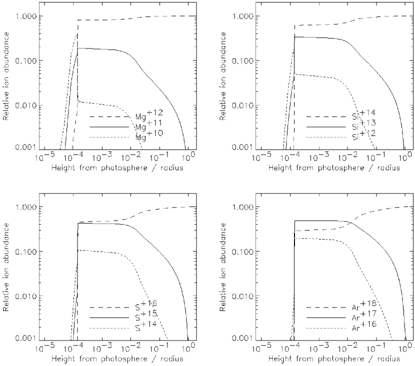
Figure 16: Vertical distribution of mid-$Z$ ions. Low charge states are omitted for clarity. The relative ion abundances are plotted against the vertical height of the atmosphere, for the disk annulus with $r=10^{11}$ cm. The thermal instability suppresses the He-like ion lines, even for the evaporating disk model, where they are strongest.

The structure of the underlying atmosphere is better discerned by plotting the height of the atmosphere above the photosphere, $z-z_{\rm phot}$. This reveals the presence of fine structure, in particular a region emitting lines from low-Z He-like ions at $T\sim 5\times 10^{4}$ K (Fig. 13 and 14). The evaporating and condensing disk model solutions (section 4) are shown in Figures 10 through 14. This low-Z He-like ion region is small due to the rapid increase in continuum opacity with decreasing temperature, but is resolved by the adaptive step-size integration. A more extended, $T\sim 10^{6}$ K region emits predominantly H-like ion and mid-Z He-like ion RR lines. Both H-like and He-like ion emission regions can be identified by the abundance distribution of the fully ionized and H-like ions, which recombine to produce the H-like and He-like ion emission, respectively (Fig. 15 and 16). The recombination line luminosity for a $u\to l$ transition in ion $Z^{+i}$ is $dL_{u\to l}\propto n_{\rm e}n_{z,i+1}T^{-\gamma}dV$ (eq. [A9] and eq. [A10]). The highest emissivities will be produced at low temperatures and high densities. This implies the region of origin of the emission will track the abundances from Figures 15 and 16, with an added bias towards the lower range of heights, which are denser and colder.

The spatial distribution of K and L-shell Fe ions shows that the structure calculation included all the intermediate ionization states (Fig. 17). The ionization parameter $\Xi$ varied continuously with atmospheric height from full ionization at $\Xi\sim 10^{3}$, down to the thermal instability regime at $\Xi\sim 10$, where a break occurs.

The presence of the instability has a large effect on the luminosity of He-like ion lines from mid-Z elements, as can be seen from Figure 16. In particular, the Mg⁺¹¹ abundance is never allowed to peak, such that the model predicts a dim Mg XI line. A similar effect occurs with Si XIII and Ne IX. Thus, in the context of this disk model, the brightness of these three lines will determine whether the instability is operating as modeled.

The discontinuity in the density, temperature, and ionization state is a result of enforcing the thermal stability of the chosen solutions, since a range of temperatures from $\sim 6\times 10^{4}$ K to $\sim 7\times 10^{5}$ K is unstable (see section 4). The discontinuity is unphysical, of course, and can be smoothed in future models by the inclusion of conduction, or any other heat transport mechanisms in the disk that might be present, such as those due to turbulence or convection.

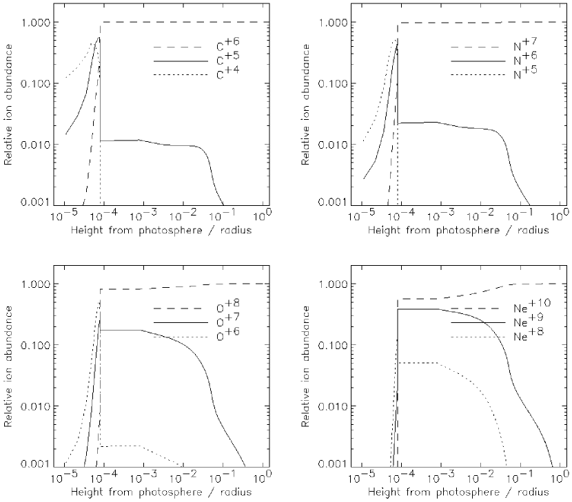
Figure 18: Vertical distribution of low-$Z$ ions for the condensing disk model. Low charge states are omitted for clarity. The relative ion abundances are plotted against $(z_{\rm atm}-z_{\rm phot})/r$, the vertical height of the atmosphere, for the disk annulus with $r=10^{11}$ cm, which dominates line emission.

A comparison of the spatial ion distribution from the condensing disk (Fig. 18) and the evaporating disk (Fig. 15) shows that the differences in the synthetic spectra can be attributed to differences in the vertical disk structure. The low-Z He-like ion line producing region shrinks, while the H-like ion line and mid-Z He-like ion line producing region expands in the condensing disk model, as compared to the evaporating case. The condensing solution shows a more extended Fe L emission region, with particularly large ion emission measure for Fe⁺¹⁹, which recombines to Fe⁺¹⁸ and produces strong Fe XIX lines (Fig. 17[b]), while the evaporating disk shows a larger emission measure for Fe⁺¹⁷ at lower temperatures (Fig. 17[c]), which recombines to Fe⁺¹⁶ and emits the Fe XVII lines more efficiently, as will be shown in section 7. This behavior traces back to the choice of solutions from the stability curve in section 4.

7 Spectroscopy

In this section we delineate the circumstances under which the disk emission is rendered observable, and we describe the disk spectroscopy and its diagnostics.

The LMXB photon net flux (photon cm^-2 s^-1 keV^-1) is modeled by:

$$F_{E}^{\rm tot}=e^{-\sigma_{E}N_{H}^{*}}F_{E}^{*}+e^{-\sigma_{E}N_{H}^{\rm disk}}F_{E}^{\rm disk}$$ (18)

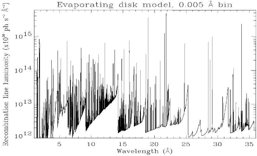
Figure 19: Modeled recombination emission from the disk atmosphere ($L_{\nu}^{\rm disk}\equiv d^{2}E^{2}F_{E}^{\rm disk}$). Neither the ionizing continuum, interstellar absorption, nor Doppler broadening are included.

where $F_{E}^{*}$ is the neutron star continuum, $F_{E}^{\rm disk}$ is the RR line and RRC modeled flux (Fig. 19), $N_{H}^{*}$ and $N_{H}^{\rm disk}$ are the neutral hydrogen absorption column densities, $E$ is the photon energy, and $\sigma_{E}$ are the Morrison & McCammon (1983) absorption cross sections. The system is assumed to be $d=10$ kpc away.

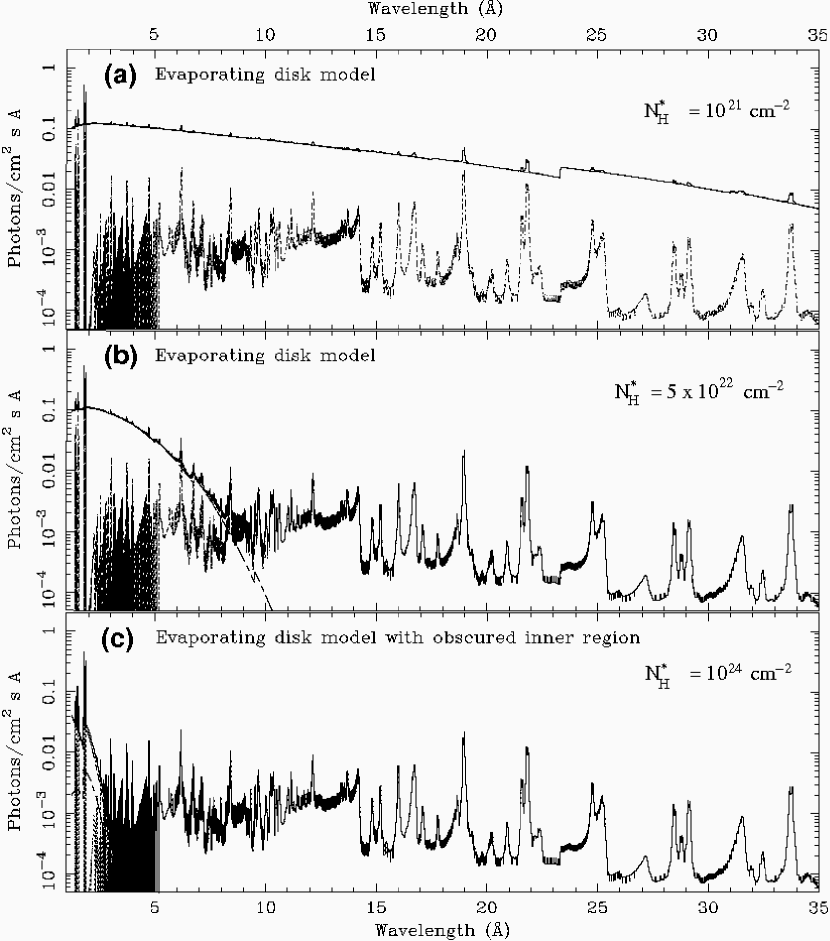
Figure 20: Model spectrum of an LMXB, with $\Delta E_{\rm x}=2$ eV bins. The line luminosity from Fig. 19 is Doppler shifted by the projected local orbital velocity, at an inclination of $75\hbox{${}^{\circ}$}$. For the disk lines, we let $N_{H}^{\rm disk}=10^{21}$ cm^-2 be constant. For the neutron star continuum, we let (a) $N_{H}^{*}=10^{21}$ cm^-2, (b) $N_{H}^{*}=5\times 10^{22}$ cm^-2, and (c) $N_{H}^{*}=10^{24}$ cm^-2. Each term in eq. (18) is shown, as well as their sum (evaporating disk model).

We find that the lines are swamped by the continuum for cases where the neutral column densities for the neutron star and the disk are set equal, or $N_{H}^{*}=N_{H}^{\rm disk}$ in eq. [18] (see the spectrum in Fig. 20[a]). This situation is most likely to occur in LMXBs with inclination in the range $i=0\hbox{${}^{\circ}$}$–$60\hbox{${}^{\circ}$}$ Frank, King, & Lasota (1987). The inclination angle $i$ is defined in Figure 1. Moreover, the continuum X-ray emission from the inner disk ($r<10^{8.5}$ cm) has been neglected here, which according to a model by Stella & Rosner (1984), will soften the continuum below $\sim 10$ Å, and this will further reduce the equivalent widths of the X-ray emission lines from the outer disk. In the inner disk, radiation pressure dominates and the SS73 viscosity prescription must be modified (Stella & Rosner, 1984). Thus, low inclination neutron star LMXBs are unlikely to have detectable X-ray lines from the disk.

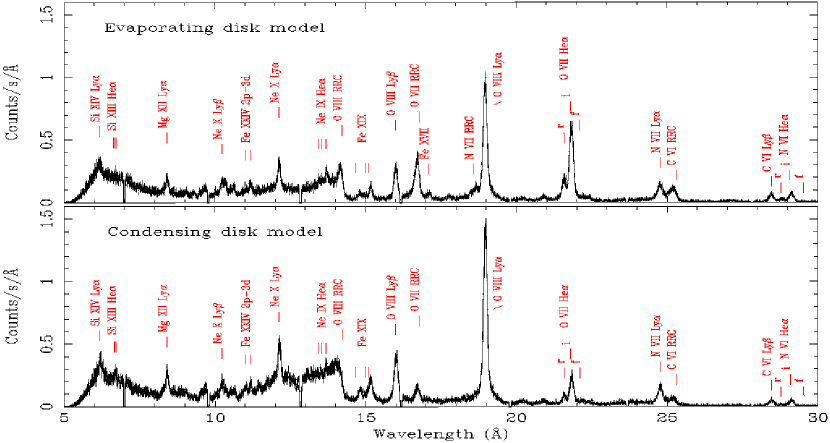
Figure 21: Spectra for evaporating and condensing accretion disks. Simulated 50 ks observation with XMM-Newton RGS 1. The evaporating disk spectrum here corresponds to Fig. 20(b). The continuum emission from the inner ($r<10^{8.5}$ cm) disk is not included, and the obscuration of the ionizing continuum from the compact object is assumed.

Thus, consider $N_{H}^{*}=5\times 10^{22}$ cm^-2 and $N_{H}^{\rm disk}=10^{21}$ cm^-2 with $i=75^{\circ}$, where an obscuring medium absorbs half of the continuum flux from the neutron star. Such a medium is compact enough to leave the disk almost unobscured (see Fig. 20[b]). This situation should arise in LMXBs which exhibit flux dips, for example, where either the disk rim or small clouds obscure the central continuum periodically, as explained in section 2.1. These LMXBs have inclinations in the $60\hbox{${}^{\circ}$}$ to $80\hbox{${}^{\circ}$}$ range (Frank, King, & Lasota, 1987). With a partially obscured central continuum, disk evaporation has an observable spectral signature. We simulated 50 ks observations with the XMM-Newton RGS 1 and the Chandra MEG (Fig. 21 and 22). Some bright lines are listed on Table 1. The evaporating and condensing disks have contrasting O VII/O VIII and Ne IX/Ne X line ratios. The evaporating disk contains gas at $T\sim(7$–$10)\times 10^{4}$ K, unlike the condensing disk. The H-like ion line intensities are higher for the condensing disk since it has more gas at $T\sim 10^{6}$ K. The spectral differences stem from the distinct differential emission measure distributions $d(EM)/d\log\Xi$ and from the O VII recombination rate $\alpha_{RR}\propto T^{-\gamma}$, where $\gamma=0.7$–$0.8$, and $EM=\int n_{z,i}n_{e}dV$ is the emission measure (appendix A).

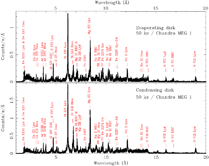
Figure 23: Evaporating and condensing disk spectra with occulted neutron star. Simulated 50 ks observations with the Chandra medium energy grating $MEG$, +1 order. The evaporating disk spectrum shown corresponds to the model in Fig. 20(c), with the neutron star practically occulted by $N_{H}^{*}=10^{24}$ cm^-2.

In the case the central continuum is completely occulted, the model predicts that numerous hard X-ray lines will become detectable with Chandra (Fig. 20[c]), such that evaporating and condensing disk models are distinguishable. Figure 23 contrasts the Chandra MEG +1 simulations of the evaporating and condensing disk models. The column density for the neutron star continuum is taken as $N_{H}^{*}=10^{24}$ cm^-2, and $N_{H}^{\rm disk}=10^{21}$ cm^-2 for the disk. Notably, the He-like to H-like ion line ratios still serve to differentiate the models at larger $Z$, but with the reverse effect. The He-like/H-like ion line ratios for Ar, S, and Si are larger for the hotter, condensing disk. The Mg XI/Mg XII ratio is roughly the same for either model. The $Q\equiv$(Fe XXV + Fe XXVI)/Si XIV line ratio is 50 % larger for the evaporating disk model. Since Fe XXV and Fe XXVI lines originate near or at the hot corona, where the instability in question does not operate, no difference in their line fluxes is observed. Since the hot atmosphere (or “warm corona”) of the condensing disk is larger than the evaporating case, more Si XIV line emission is produced, and the $Q$ ratio is smaller. This shows that the way the thermal instability is treated in the models (in this case, whether we pick the evaporation or condensation solutions), has a dramatic effect on all the line ratios which are sensitive to the ionization distribution.

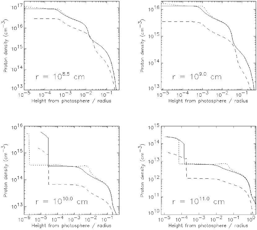
Figure 14: Modeled proton density ($n_{p}$) vs. disk atmosphere height above the photosphere ($z_{\rm atm}-z_{\rm phot}$) for various radii. Evaporating (solid line), condensing (dotted line), and low-luminosity (dashed line) disk models. The height is normalized to the local radius.

The He$\alpha$ line triplets can be used as density diagnostics, but they may be affected by photoexcitation by the UV field from the accretion disk (Gabriel & Jordan, 1969; Blumenthal, Drake, & Tucker, 1972). The forbidden line $f$ of O VII at $22.097$ Å is suppressed due to collisional depopulation at high density, since $n_{e}\gtrsim 10^{14}$ cm^-3 (see the density profiles in Fig. 14 and the O⁺⁷ relative abundance distribution in Fig. 15). The O VII intercombination $i$ to resonance $r$ line ratio is $g=(f+i)/r\simeq i/r\gtrsim 4$, indicating a purely photoionized plasma (Porquet & Dubau, 2000). The O VII and N VI He$\alpha$ line ratios are included in the model at their high-density limit, while the He$\alpha$ line ratios of other ions such as Si XIII have not been modeled yet, since the line ratios will start to be a function of position in the atmosphere, adding complexity. The depopulation of the forbidden line in many He-like ions was attributed to resonant photoexcitation in Hercules X-1 (Jimenez-Garate et al., 2002). The intense UV fields in LMXBs imply the same effect will operate (Liedahl et al., 1992). In the context of the present model, the region where He-like ions are abundant is very close (less than $10^{7}$ cm away) to the photospheric surface, such that the UV energy density is as high as in the photospheric surface. This implies that the He-like diagnostics will be degenerate to high density and UV field effects (cf., Mauche, Liedahl, & Fournier, 2001).

The optical depth of the atmosphere may be probed by comparing the observed spectra to the model, which assumes the lines are optically thin. In particular, the O VII $r$ line may differ from the modeled value due to resonant scattering of continuum photons. Whether $r$ gets enhanced or absorbed depends on geometry and the relative placement of emissivity and opacity. The $i$ and $f$ lines should be optically thin, so optical depth can modify the $g$ ratio substantially from $g\sim 4.2$, the value expected for a photoionization-dominated, optically thin gas. The Ly$\alpha$ line in hydrogenic ions also has a large scattering cross section. Thus, the He$\alpha$ $r$ and/or Ly$\alpha$ lines are good indicators of optical depth.

The RRC can be used for temperature diagnostics, and also for probing the behavior of the thermal instability. The local RRC width $\propto T$ (Liedahl & Paerels, 1996). The O VII RRC broadening is Doppler-dominated, resembling the RR lines, for both the evaporating and condensing cases. The O VIII RRC shape varies noticeably from the evaporating to the condensing condition. In the evaporating case, the O VIII RRC has two temperature components, one with a $FWHM\sim 2$ Å that is produced at $T\sim 10^{6}$ K, and another narrow component with $T\sim 10^{5}$ K. The two components are distinguishable because intermediate temperatures are thermally unstable. Thus, the RRC profile in this case provides evidence for the existence of this thermal instability. In the condensing case, the RRC has a single, broad temperature component at $T\sim 10^{6}$ K, since the disk atmosphere temperature suddenly drops from the latter value to one where the X-ray emission is negligible. The broadening of this RRC is also peculiar, since RRC are usually narrow for all photoionized gases, given that the kinetic energy of the gas particles is generally much smaller than the recombining photon energy (Liedahl & Paerels, 1996).

7.1 Luminosity Dependence

The disk model was run with a lower central luminosity $L=0.1L_{\rm Edd}$, for comparison to the $L_{\rm Edd}$ case explored in the previous sections, to investigate the structural and spectral changes of the disk.

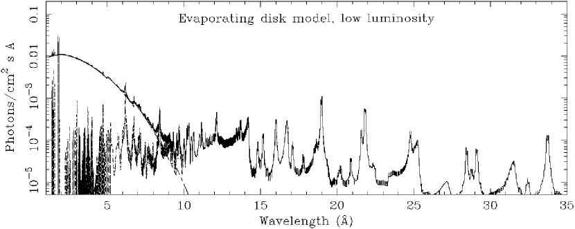
Figure 24: Model spectrum of an LMXB with $L=0.1L_{\rm Edd}$, with $\Delta E_{\rm x}=2$ eV bins. Doppler shifts from the projected disk orbital velocity is included at an inclination of $75\hbox{${}^{\circ}$}$. The disk emission has $N_{H}=10^{21}$ cm^-2, and the continuum emission has $N_{H}^{*}=5\times 10^{22}$ cm^-2. Compare to the $L_{\rm Edd}$ case in Fig. 20(b).

The atmospheric radiative recombination luminosity was $\sim 20$ times lower than the $L=L_{Edd}$ case, indicating a nearly linear dependence of the disk luminosity to the central luminosity. Otherwise, the low-luminosity spectrum shown in Figure 24 shows much resemblance to its $L_{\rm Edd}$ counterpart. The dependence of the recombination luminosity can be approximated by

$$L_{u\rightarrow l}\propto L_{\rm x}\frac{\Omega}{4\pi}$$ (19)

where $\Omega$ is the solid angle subtended by the disk atmosphere. This relationship is then modified by the changing density, opacity and thickness of the atmosphere. To explain the recombination luminosity behavior, we will first describe the calculated atmosphere structure.

The photospheric and atmospheric boundaries were fitted by power laws. The fit parameters defined in section 6 were $C_{\rm phot}=(1.8\pm 0.3)\times 10^{-3}$ cm, $n_{\rm phot}=1.14\pm 0.01$, $C_{\rm atm}=(1.2\pm 0.2)\times 10^{-3}$ cm, and $n_{\rm atm}=1.18\pm 0.01$. The fit errors are shown, while systematics are expected to follow the same trends as in section 6. The solid angle subtended by the entire disk $\Omega/4\pi\simeq 0.1$, while for the Eddington Luminosity case $\Omega/4\pi\simeq 0.2$, as can be seen by comparing Figure 9 with Figure 25. This implies little variation of the disk shape with luminosity. With a factor of ten reduction in luminosity, the radiative energy incident on the disk is 20 times smaller, which coincides with the observed reduction in the recombination emission.

The accretion disk structure for $0.1L_{\rm Edd}$, shown in Figures 10, 11, 13, and 14, yields a density $\sim 4.5$ times smaller than the $L_{\rm Edd}$ case. Aside from the density change, the ionization structure remains quite similar to the $L_{\rm Edd}$ case (see Fig. 17[a] and 17[b]). Naively, a factor of 10 decrease in the density would be expected to keep $\xi$ constant. However, since the atmospheric volume shows little change, the observed density change implies a factor of $\sim 20$ decrease in the ion emission measure, verifying the consistency of the density with the modeled recombination flux.

We reconcile $\xi$ with the larger-than-expected density of the atmosphere by accounting for a decrease in the atmospheric opacity. Considering $\xi$ to be constant, such that

$$\xi\propto\frac{e^{-\tau(n)}L_{\rm x}}{n}=\frac{e^{-\tau(n^{\prime})}L_{\rm x}^{\prime}}{n^{\prime}}$$ (20)

where $\tau(n)\propto n$, implies that a decrease in density decreases the opacity, which increases the local flux in the atmosphere. Thus, the overdensity of the atmosphere is explained by a factor of $\sim 2$ decrease in $e^{-\tau}$, which was verified in the models. For the $L=0.1L_{\rm Edd}$ case, the atmosphere transmits 34 % of the incident flux directly for a disk annulus with $r=10^{11}$ cm, i.e. $\int F_{\nu}(z_{\rm phot})d\nu/\int F_{\nu}(z_{\rm cor})d\nu\sim 0.34$, compared to 12 % in the $L=L_{\rm Edd}$ case (see section 6). The atmospheric opacity is a function of radius, but the observed spectra are weighted towards the largest radii.

The argument above holds for plane parallel atmospheres that are photoionized by radiation incident at a small grazing angle $\theta\ll 1$, such that $\tau\sim 1$ for a grazing ray, but $\tau\ll 1$ for any other ray. Therefore, the recombination luminosity will be proportional to the total emission measure for most viewing angles.

As more of the X-ray continuum is transmitted onto the disk photosphere, the heating of the optically thick disk increases. This effect is taken into account to derive a self-consistent midplane disk temperature, to 10 %. The input grazing angle and the grazing angle calculated from $z_{\rm atm}$ are consistent at the 25 % level.

7.2 A weak coupling between the disk and its atmosphere

There is a negligible change in the atmospheric structure by varying $\alpha$ from 0.1 to 1 in the disk model. As explained below, this can be understood as a decoupling which exists between the optically thick disk and the photoionized atmosphere.

The viscosity parameter $\alpha$ has no effect on the disk temperature, but it does on the density, since $\rho\propto\alpha^{-1}$ (SS73). Assuming vertical isothermality in the optically thick disk (below the photosphere), its pressure can be obtained from equation (3) and is given by:

$$P(z)=P_{\rm o}e^{-z^{2}/2Z_{\rm P}^{2}}$$ (21)

with $P_{\rm o}\propto\alpha^{-1}$. The photoionized atmosphere is placed on top of this disk, and satisfies two boundary conditions: matching temperature and pressure at the photospheric boundary. Assume the base of the atmosphere is at some pressure $P_{\rm phot}$, and let a change in viscosity from $\alpha$ to $\alpha^{\prime}$ produce a change in the subphotospheric disk pressure from $P_{\rm o}$ to $P_{\rm o}^{\prime}$. To match the boundary conditions, the atmosphere has to shift in height, such that

$$P_{\rm phot}=P_{\rm o}e^{-z^{2}/2Z_{\rm P}^{2}}=P_{\rm o}^{\prime}e^{-(z^{\prime})^{2}/2Z_{\rm P}^{2}}$$ (22)

which implies that the height shift in the atmosphere, $\Delta z=z^{\prime}-z$, is given by:

$$\frac{\Delta z}{z}\simeq\frac{Z_{\rm P}^{2}}{z^{2}}\ln\Biggr{(}\frac{P_{\rm o}^{\prime}}{P_{\rm o}}\Biggl{)}=\frac{Z_{\rm P}^{2}}{z^{2}}\ln\Biggr{(}\frac{\alpha}{\alpha^{\prime}}\Biggl{)}$$ (23)

where the approximation $z^{2}\gg Z_{\rm P}^{2}$ was used, which is valid since $z_{\rm phot}>3Z_{\rm P}$ in the models for $\alpha<1$. In such a case, it follows that $\Delta z/z\ll 1$, so that very large changes in viscosity only produce minute shifts on the atmospheric height and negligible effects on the atmospheric emission (as already pointed out by Nayakshin, Kazanas & Kallman (2000)).

There are, however, other situations where the role of dissipation in the atmosphere has to be reassessed: 1) if the dissipated energy in the disk is no longer negligible compared to the exterior illumination energy, as might be the case for disks around black hole candidates, and if energy is transported to the atmosphere via magnetic flares, for example, and 2) if there is negligible dissipation, but it is sufficient to enhance mixing and, therefore, change the atmospheric structure.

Różańska, Dumont, Czerny, & Collin (2002) noted that the structure of the optically-thick disk has non-negligible effects in the corona when the disk scale height is comparable to or larger than the coronal scale height (in our notation, when $Z_{\rm P}\gtrsim z_{\rm cor}$). This does not apply to our case, because for a neutron star LMXB disk with $r>10^{8.5}$ cm, we get $z_{\rm cor}\gg Z_{\rm P}$. Różańska, Dumont, Czerny, & Collin (2002) assert that the disk and corona are coupled in BHC for $r\sim 10~{}R_{\rm G}$, where $R_{\rm G}$ is the Schwarzschild radius; while for AGN, the situation depends on the accretion rate. By this measure, the disk-corona coupling may also be significant in the outer radii of BHC disks, if the reduction of the central illumination flux shrinks the size of the corona.

7.3 Emission line profiles

Synthetic profiles were produced for all the emission lines. For simplicity, the calculation assumes that line scattering is negligible, which may not be a valid assumption for resonance lines. Here we select the profiles of the brightest lines that are not contaminated by other ions. The line profiles are also calculated for a disk within the $10^{8.5}<r<10^{10}$ cm radius range, for comparison with the $10^{8.5}<r<10^{11}$ cm radius range shown above. The emission line profiles have more broadly separated peaks for smaller disks, as shown in Figure 26.

No variation in line broadening is obtained as a function of charge state. The N VI Ly$\alpha$ line has the same velocity profile as the corresponding lines in O VIII, Ne X, Si XIV, and Fe XXVI. We attribute this to the vertical stratification of the atmosphere, which allows the full range of ionization parameters detectable in the X-ray band to exist in every annulus. Future two-dimensional models taking into account radiation transfer in the radial direction may exhibit a trend for the line widths, since the radial optical depth is not negligible.

8 Discussion

8.1 Neutron star LMXB spectra observed with Chandra and XMM-Newton

The LMXB spectra observed with the Chandra High Energy Transmission Grating (HETG) and the XMM-Newton RGS already provide stringent tests for the models in this article. The high resolution spectra of LMXBs are generally dominated by continuum emission, which is sometimes punctuated by emission or absorption lines. Only a fraction of the sample of observed neutron star LMXBs show prominent lines. The accreting pulsar 4U1626-67 shows double-peaked and broad emission lines Schulz et al. (2001). The eclipsing dipper EXO0748-67 has broad emission lines Cottam et al. (2001a). The accretion disk corona source 4U1822-37 has narrow emission lines Cottam et al. (2001b). The dipper source 4U1624-49 shows narrow absorption lines Parmar, Oosterbroek, Boirin, & Lumb (2002). Her X-1, an intermediate-mass X-ray binary with a precessing accretion disk, has narrow emission lines during its low- and intermediate-flux states Jimenez-Garate et al. (2002). The line emission spectra are dominated by H-like and He-like ions. P Cygni profiles are observed in Circinus X-1 Brandt & Schulz (2000), a unique LMXB with high-velocity outflows. Most LMXBs do not exhibit discrete spectral features aside from interstellar absorption, such as X0614+09 Paerels et al. (2001). The emerging pattern implies that at least three classes of neutron star LMXBs exist which produce detectable X-ray emission lines: 1) high inclination LMXBs with $i\gtrsim 70^{\circ}$, 2) accreting X-ray pulsars, and 3) LMXBs with high velocity winds.

Our models are proving to be of great relevance to the interpretation of the spectra of LMXBs with high inclination and LMXBs with an X-ray pulsar. Most importantly, all LMXB spectra validate the basic assumption in our model: the plasma is photoionized. Evidence for other heating mechanisms, such as shocks, is not observed in LMXB spectra. Shocks are predicted by the Miller & Stone (2000) MHD disk models, but it is not clear whether X-ray emission from such shocks would be observable. The observed signatures of a plasma heated primarily by photoionization are the RRC, the peculiar He$\alpha$ line ratios, and the weakness of Fe L line emission relative to that of low-Z and mid-Z elements Liedahl (1999). The spectra have prominent line emission from H-like and He-like ions. These properties are shared by all the spectra shown in this article. Furthermore, the line velocity broadening observed in two LMXBs (4U1626-67 and EXO0748-67) provides kinematic evidence for accretion disk atmospheric and coronal emission.

By contrast, our model is inadequate for the interpretation of the spectra of LMXBs with high-velocity winds. These spectra show a photoionized gas with significant optical depth. Circinus X-1 is rare because of the extreme gas dynamics and the sizable line optical depths which are evident in its spectrum. The density $n_{e}\sim 10^{13}$ cm^-3 deduced from the observed P Cygni profiles in Circinus X-1 Brandt & Schulz (2000) is consistent with our model calculations, but the wind dynamics rules out our assumption of hydrostatic equilibrium. The modeling of an LMXB disk wind spectrum requires a wind acceleration mechanism and a revised disk structure Proga & Kallman (2002).

Initially, our model can be used as a tool for the identification of the discrete X-ray spectral signatures from the accretion disk atmosphere and corona. Our model provides a quantitative expectation of the X-ray line fluxes produced by the entire disk. Our physical calculation of the line profiles (and therefore the line emissivity as a function of $r$), can be used to measure the maximum disk radius and the radial ionization distribution. Furthermore, we have modeled the density at which each ion is produced, and this is testable with plasma diagnostics. The ionization distribution (measured by the flux of the emission from the high-ionization species relative to that of the low-ionization species) is a fingerprint of the disk atmosphere and corona. The temperature structure of the disk atmosphere can also be probed with the temperatures measured with the RRC of various ions. A full investigation of the models as compared with spectral data will be performed in a future paper.

8.2 Limitations of the model

The disk structure can be improved by relaxing the assumptions made in the radiation transfer calculations. The spectral model calls for the inclusion of additional lines. The observed spectra will also allow us to investigate additional physics in the disk which may be missing in our current model.

A 2-D or 3-D transfer calculation is needed to improve the coronal structure model. To simplify the radiation transfer calculations, we split the disk into a set of nested cylindrical shells, and we use 1-D transfer to calculate the structure of each shell. By defining $z_{\rm atm}(r)$ and iterating on $\theta(r)$ in each shell until self-consistency is obtained (see eq. [8] and Fig. 5), we produce a pseudo-2-D transfer calculation. However, the 1-D transfer approximation starts to break down at the largest radii, since $z_{\rm cor}\sim r$ at $r\gtrsim 10^{10}$ cm (see Fig. 10).

The UV emission is included in the structure model but remains to be added to the high resolution spectral model. However, we do not expect substantial differences between the UV spectrum obtained with our disk model and the results by Raymond (1993). The optical depth of UV lines such as C IV is $\sim$100 in the latter model. The UV and optical lines originate just above the photosphere ($z_{\rm phot}$), at densities of $10^{13}<n_{e}<10^{14}$ cm^-3. The structural difference between our models and those by Raymond (1993) occurs at the X-ray emitting atmosphere and corona. In contrast, the $z_{\rm phot}(r)$ in our models agrees well with those by Raymond (1993).

Fluorescence and resonant scattering will need to be added in the spectral model. The fluorescence line flux can be of the same order as the recombination line flux. The $r$-dependence of the Fe K fluorescence flux should be distinct from the $r$-dependence of the recombination emission. A 6.4 keV Fe K emission line is produced by M-shell charge states of Fe localized at the base of the atmosphere (see Fig. 17). The Fe K fluorescence flux will scale with the hard X-ray transmittance of the atmosphere and corona.

The structure model indicates that the optical depth of resonance lines is large. However, a realistic treatment of resonant scattering in our spectral models is complicated by the velocity shear within the disk. Resonant scattering and Fe K fluorescence emission were only included in the low-resolution 1-D transfer calculations to obtain the disk structure. The propagation of resonance line photons is highly anisotropic, and it depends on the viewing angle because of the Keplerian velocity shear and the geometrical thickness of the atmosphere. LMXBs with strong emission lines do not exhibit detectable features from resonant scattering of continuum photons, with the exception of Circinus X-1 (section 8.1).

Magnetic fields, which are not included in our model, may affect the structure of some regions of the disk (see section 8.3).

8.3 A strongly magnetized corona?

A strong magnetic field may affect the coronal structure and the X-ray spectrum. The corona under consideration is located at the outer radii of a centrally illuminated disk. We believe $B$ fields play a secondary role in this type of corona, because the energy budget of the corona is dominated by X-ray irradiation. In detail, the role of $B$ fields cannot be discounted, because phenomena such as magnetic flare heating may dominate over photoionization within localized regions of the disk. Recent MHD models predict $B$ fields larger than the virial value in the disk corona. However, the applicability of these MHD models to the illuminated corona is dependent on the effects of radiative heating and magnetic reconnection.

MHD models of radiationless accretion disks show that above a few scale heights, the magnetic pressure is larger than $P_{\rm gas}$ Miller & Stone (2000). The gas dynamics in the disc is dominated by the $MRI$. Miller & Stone (2000) found that the $MRI$ produces $B$ fields which buoyantly rise to the atmosphere and corona. In their model, 25% of the magnetic energy generated by the $MRI$ rises to the corona, representing 60% of the local heating, but $\lesssim 4$% of the dissipative heating in the disk. A 3D MHD disk model by Machida, Hayashi, & Matsumoto (2000), with an initial toroidal configuration, shows that the strong $B$ fields in the corona are confined in filaments, with a filling factor of a few percent. Another 3D MHD model by Hawley, Balbus, & Stone (2001) confirms the presence of large $B$ fields in the corona.

By contrast, when X-ray illumination is present, the $B$ field plays a relatively minor role in the overall energetics of the disk corona. This is true at least in a spatially-averaged sense. The magnetic energy produced by the $MRI$ can be no larger than the energy dissipated in the disk. The maximum energy available for the $B$ field scales as $r^{-3}$, and it is given by the first term on the right side of equation (1). Assuming all of the accretion energy is contained in the $B$ field, equation (2) indicates that the illumination energy is larger than the magnetic energy for $r\gtrsim 10^{10}$ cm (per unit disk area). Since MHD disk models typically assume an isothermal or adiabatic disk, they may not apply to an extended hot corona dominated by photoionization.

Magnetic reconnection has the effect of decreasing the magnitude of the disk-coronal $B$ field. Coronal flares resulting from magnetic reconnection convert magnetic energy into kinetic energy through particle acceleration. Most of the X-rays in black hole accretion disks may be produced by magnetic flares di Matteo (1998). In the Liu, Mineshige, & Shibata (2002) model, reconnection events in disk flares reduce the $B$ field by a factor of $\sim 30$. Thus, the buoyant $B$ field may be dissipated in a flaring region.

9 Conclusions

We have calculated the hydrostatic structure of a photoionized accretion disk atmosphere which is in thermal equilibrium and ionization balance. We also determined the atmosphere’s thermal stability and its observable high resolution X-ray recombination emission spectrum.

• A feedback mechanism between illumination and atmospheric structure enlarges the atmosphere. The disk atmosphere is orders of magnitude less dense than the disk midplane. The atmosphere extends for a few tens of disk pressure scale heights (if the pressure scale height is calculated using the disk midplane temperature). Illumination heats and expands the disk atmosphere, increasing the number of absorbed photons in the atmosphere and heating it further, producing further expansion of the atmosphere, and so on. The expansion stops because the atmosphere becomes optically thin, cooling and contracting. The inclusion of the feedback mechanism increases the size and the line emission flux of the atmosphere by an order of magnitude. The atmospheric thickness is much larger than the standard $\alpha$-disk model thickness, and it is consistent with the $\sim 12\hbox{${}^{\circ}$}$ subtended semi-angle deduced from optical modulations in LMXBs. The disk atmosphere thickness also explains the under-abundance of eclipsing LMXBs.

• The disk atmosphere subtends a large solid angle $0.07\lesssim\Omega/4\pi\lesssim 0.2$. If the inclination is $i\gtrsim 80\hbox{${}^{\circ}$}$, the disk photosphere (which subtends $0.04\lesssim\Omega/4\pi\lesssim 0.08$) may shield the neutron star flux, producing an ADC source with partial eclipses or without eclipses altogether. The disk $\Omega$ depends weakly on the neutron star luminosity, but $\Omega$ scales linearly with disk radius. The disk recombination luminosity scales linearly with $\Omega$.

• The atmospheric structure is independent of the viscosity parameter $\alpha$. The viscosity changes the density in the optically-thick part of the disk, producing a small shift in atmospheric height, but this has no effect on the X-ray spectrum.

• The X-ray spectra are dominated by lines from H-like and He-like ions of abundant elements from C to Fe, as well as RRC and weak Fe L lines. The line ratios are a sensitive probe of the atmospheric and coronal structure.

• Clear spectral signatures of photoionization are present, as well as temperature, density, and radiation field diagnostics. An intercombination to resonance line ratio of $\sim 4$ is modeled for low-Z He-like ion line triplets. RRC are unequivocal signposts of photoionization. The density diagnostics from He$\alpha$ lines of low-Z and intermediate-Z elements are degenerate with the presence of an intense UV radiation field from the disk itself, so the $R$ ratio may not give conclusive signatures of high-density in LMXBs. Much of the disk atmosphere is close to the photosphere, such that the dilution factor of the UV field is small. The He$\alpha$ density diagnostics could operate at the densities predicted by the disk atmosphere model in LMXBs, of $10^{13}\lesssim n_{e}\lesssim 10^{15}$ cm^-3.

• The line fluxes are nearly proportional to the X-ray continuum luminosity. The disk line fluxes decreased by a factor of 20 when the system luminosity was decreased by a factor of 10 (to $L=10^{37.3}$ erg s^-1). The atmospheric density was reduced by a factor of $\sim 5$, its optical depth was reduced, and the atmosphere was $\sim 2$ times less extended than in the high-luminosity ($L=10^{38.3}$ erg s^-1) case.

• The line equivalent widths depend strongly on inclination. The relative obscuration of the neutron star affects the equivalent width and detectability of the disk X-ray emission. The modeled disk emission is almost undetectable when the neutron star continuum is also in the line of sight. As such, high inclination systems, or systems with dips or ADC, are more likely to show X-ray lines due to enhanced contrast. This expected trend has been largely confirmed by Chandra and XMM-Newton observations. We have demonstrated that for a highly absorbed neutron star continuum in our fiducial system, the disk X-ray lines are detectable with both the Chandra and XMM-Newton grating spectrometers.

• Double-peaked X-ray lines can be detected for $r=10^{10}$ cm disks, but larger $r=10^{11}$ cm disks may appear blended in a single peak in the grating spectra. The emission line region spans several orders of magnitude in disk radius. The modeled line profiles are needed to deduce the outer disk radius. Line emission from the outer regions of the disk dominates. The emission increases with disk radius, and the Doppler broadening of the lines decreases for larger $r$. The wings of the broadest lines are lost in the continuum, decreasing their apparent equivalent width.

• The resonance line optical depths can be measured. If the $r$ line in He-like ions has a value which differs from the model calculations, it may be due to resonant scattering of continuum photons. The line ratios in the Lyman series can also work as optical depth diagnostics. We have not included these effects on the current version of the model, but our results for ionic column densities show that appreciable line optical depths are present, and hence this process will be included in future versions of the code.

• The continuum optical depth of the atmosphere is generally small ($\tau\ll 1$), except for photons which propagate nearly parallel to the disk plane. The atmosphere is optically thick to X-ray continuum photons from the neutron star. However, most of the recombination line emission is not appreciably affected by the continuum opacity.

• The spectrum is sensitive to a thermal instability present in photoionized gases. By forcing all the chosen solutions to be thermally stable, a break in the temperature, density, and ionization structure is created. Measurably different X-ray spectra are obtained depending on the resolution of this instability. The shape of RRC profiles, which in the models show multiple temperature components, and the relative intensity of lines such as Mg XI, are useful diagnostics of the stable temperature regime.

The spectra obtained with the Chandra HETG and the XMM-Newton RGS show that the plasmas in LMXBs are photoionized, as our model assumes. Two LMXBs (4U1626-67 and EXO0748-67) show kinematic signatures of accretion disk emission Schulz et al. (2001); Cottam et al. (2001a). The line fluxes, line profiles, the ionization distribution, density, and RRC temperatures, provide a wealth of diagnostic capability for the identification of accretion disk atmospheres and their properties. The spectral comparisons with the data are promising, and they will be addressed in future work.

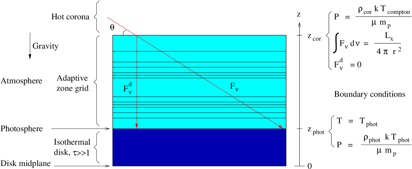
Figure 3: Gas column geometry for each disk annulus. The boundary conditions on the atmospheric structure are shown.

Figure 5: Grazing angles $\theta(r)$ for the radiation impinging on the disk, at successive model iterations (A to D). The $\theta(r)$ input to the model are compared to the $\theta(r)$ extracted from the output disk structure. The resulting model D is self-consistent and has a finer grid.

Figure 9: Total solid angle subtended by the disk photosphere ($z_{\rm phot}$), atmosphere ($z_{\rm atm}$), and corona ($T=5\times 10^{6}$ K isotherm). The atmosphere subtends a much larger solid angle than would be expected by just considering the local pressure scale height at the photospheric temperature ($H_{\rm P}=Z_{\rm P}$).

Figure 17: Vertical distribution of K and L-shell ions of Fe, plotted for: (a) the condensing disk with $L=L_{\rm Edd}$, (b) the evaporating disk with $L=L_{\rm Edd}$, and (c) the evaporating disk with low-luminosity ($0.1L_{\rm Edd}$). The relative abundances are plotted vs. the height $(z_{\rm atm}-z_{\rm phot})/r$, for the disk annulus with $r=10^{11}$ cm. The plateau and break at $(z_{\rm atm}-z_{\rm phot})/r=0.0001$–$0.003$ correspond to the instability regime.

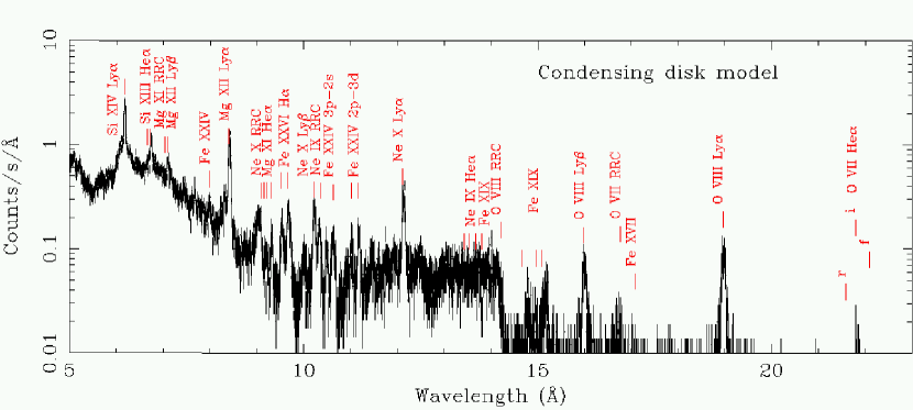
Figure 22: Condensing disk spectrum (as in Fig. 21). Simulated 50 ks observation with Chandra $MEG$, +1 order.

Figure 25: Total solid angle subtended by the disk photosphere ($z_{\rm phot}$), atmosphere ($z_{\rm atm}$), and corona ($T=5\times 10^{6}$ K isotherm). The disk structure for the low-luminosity ($L=0.1L_{\rm Edd}$) case is shown, whose atmosphere subtends a solid angle 30 to 40 percent smaller than the $L=L_{\rm Edd}$ case on Fig. 9.

Figure 26: From top to bottom and left to right: line profiles for N VI He$\alpha$, N VII Ly$\alpha$, O VII He$\alpha$, O VIII Ly$\alpha$, Ne X Ly$\alpha$, and Si XIV Ly$\alpha$. The bin size is $\Delta\lambda=0.005$  Å. The solid line corresponds to a disk with maximum radius of $r=10^{11}$ cm, while the dashed line is the weaker and broader line profile produced by a disk with $r=10^{10}$ cm.

Table 1: Line fluxes for disk models. Line fluxes in units of $10^{-12}$ erg cm^-2 s^-1, typically over an interval $E/\Delta E\sim 100$. Estimated systematic normalization error limit of $\sim 50$ %, due to the 1-D transfer calculation. These line fluxes do not include any interstellar absorption effects, unlike those from Table 1 in Jimenez-Garate, Raymond, Liedahl, & Hailey (2001).

	$L=0.1L_{\rm Edd}$	$L=L_{\rm Edd}$	$L=L_{\rm Edd}$	$L=L_{\rm Edd}$
	$r=10^{11}$ cm	$r=10^{11}$ cm	$r=10^{10}$ cm	$r=10^{11}$ cm
Line(s)	Evaporating	Evaporating	Evaporating	Condensing
C VI Ly$\alpha$	0.11	2.0	0.49	1.7
N VI He$\alpha$	0.063	1.3	0.27	0.98
N VII Ly$\alpha$	0.061	1.1	0.29	1.1
O VII He$\alpha$	0.26	5.1	1.0	2.4
O VIII Ly$\alpha$	0.36	6.1	1.9	8.4
O VII RRC	0.12	2.1	0.43	1.0
O VIII Ly$\beta$	0.087	1.47	0.46	2.3
Fe XIX L (0.815 keV)	0.038	0.67	0.22	1.4
Ne X Ly$\alpha$	0.099	1.7	0.54	2.8
Fe XXVI H$\alpha$ (1.28 keV)	0.040	0.84	0.25	0.98
Mg XII Ly$\alpha$	0.072	1.3	0.35	2.1
Si XIII He$\alpha$	0.080	1.3	0.44	2.5
Si XIV Ly$\alpha$	0.024	4.2	1.4	6.2
S XV He$\alpha$	0.066	1.3	0.47	2.5
S XVI Ly$\alpha$	0.12	2.3	0.72	3.0
Ar XVII He$\alpha$	0.061	1.3	0.46	2.5
Ar XVIII Ly$\alpha$	0.067	1.3	0.35	1.7
Ca XIX He$\alpha$	0.025	0.53	0.19	0.90
Ca XX Ly$\alpha$	0.027	0.52	0.17	0.64
Fe XXV He$\alpha$	0.91	16	4.6	16
Fe XXVI Ly$\alpha$	0.57	12	4.0	12

Appendix A Radiative Recombination Emission

We describe the numerical calculation of the radiative recombination emission, including both recombination lines and radiative recombination continua. A similar method for an optically thin gas in the photoionized wind of a High Mass X-ray Binary $HMXB$ was described by Sako et al. (1999).

Consider an infinitesimal volume $dV$ at which a single ionization parameter $\xi$, temperature $T$, electron density $n_{\rm e}$, and elemental abundances $A_{z}$ describe the state of a gas. The $\xi(T)$ function is found from thermal balance and ionization equilibrium, for a given ionizing spectrum $F_{\nu}$ (section 3.3). In the radiative recombination process

$$Z^{+(i+1)}+e^{-}\rightarrow Z^{+i*}+h\nu_{RRC}$$ (A1)

an electron recombines with an ion with net charge +$(i+1)$, assumed in its ground state, producing a new ion with net charge +$i$, which might be excited. The radiative recombination continuum photon has energy

$$E_{\rm x}=h\nu_{RRC}=\chi+KE_{e},$$ (A2)

where $\chi$ is the ionization energy of ion $Z^{+i*}$, and $KE_{e}$ is the initial kinetic energy of the electron, assumed to be on a Maxwell distribution with temperature $T$. The radiative recombination rate to $Z^{+i}$ (where $Z^{+i}$ can be in any quantum state) in units of s^-1 is

$$\Gamma_{RR}=n_{\rm e}n_{z,i+1}\alpha_{RR}dV$$ (A3)

where $n_{z,i+1}$ is the $Z^{+(i+1)}$ ion number density, equation (A3) defines $\alpha_{RR}$, the total radiative recombination rate coefficient in units of cm³ s^-1. Note $\alpha_{RR}$ depends on $Z$, $i$, and $T$.

A.1 Recombination Lines

After recombination, a fraction $\eta_{u\rightarrow l}$ of the $Z^{+i}$ ions produce a radiative cascade photon by an electronic transition from upper level $u$ to lower level $l$. The line luminosity of photons from this transition in units of erg s^-1 is

$$dL_{u\rightarrow l}=n_{\rm e}n_{z,i+1}E_{u\rightarrow l}\eta_{u\rightarrow l}\alpha_{RR}dV$$ (A4)

where $E_{u\rightarrow l}$ is the transition energy in ergs. To create a synthetic spectrum, the line luminosities $dL_{u\rightarrow l}$ at energies $E_{u\rightarrow l}$ in the X-ray band are added for all the levels $u,l$, and all the ions $Z^{+(i+1)}$ which are abundant in the gas. Notice the recombination emission of the $Z^{+i}$ ion depends on the number density of the $Z^{+(i+1)}$ ion.

For computational purposes, various quantities from equation (A4) are defined. The specific line power

$$S_{u\rightarrow l}\equiv\eta_{u\rightarrow l}\alpha_{RR},$$ (A5)

in units of cm³ s^-1, is the photon emission rate per $Z^{+(i+1)}$ ion, per unit electron density. The $Z^{+(i+1)}$ ion was assumed to be in its ground state before recombining into $Z^{+i}$. The population fraction $f_{u}$ of each level of the $Z^{+i}$ ion is computed explicitly, and $S_{u\rightarrow l}$ is obtained by equating the matrix of the photon emission rates per ion,

$$n_{\rm e}S_{u\rightarrow l}=f_{u}A_{u\rightarrow l}$$ (A6)

where $A_{u\rightarrow l}$ is the rate of spontaneous decay for $Z^{+i}$. After solving $S_{u\rightarrow l}$ for a grid of temperatures, typically in the 10 to 80 eV range, it is fit to a power law

$$S_{u\rightarrow l}=C_{u\rightarrow l}T^{-\gamma_{u\rightarrow l}}$$ (A7)

where the exponent $\gamma_{u\rightarrow l}$ is typically 0.6–0.8. The number density of $Z^{+(i+1)}$ is calculated with

$$n_{z,i+1}=n_{H}A_{z}f_{z,i+1}$$ (A8)

where $n_{H}$ is the proton density, $A_{z}$ is the fractional abundance of element $Z$ relative to $H$, and $f_{z,i+1}$ is the fractional abundance of the $Z^{+(i+1)}$ ion relative to all the $Z$ ions. The differential emission measure for $Z^{+(i+1)}$ is defined as

$$d(EM_{z,i+1})\equiv n_{\rm e}n_{z,i+1}dV,$$ (A9)

in units of cm^-3. The line luminosity in equation (A4) can therefore be re-written as

$$dL_{u\rightarrow l}=E_{u\rightarrow l}S_{u\rightarrow l}d(EM_{z,i+1}).$$ (A10)

If the emission measure is defined as $d(EM)\equiv n_{\rm e}^{2}dV$, then $dL_{u\rightarrow l}=P_{u\rightarrow l}d(EM)$, where $P_{u\rightarrow l}$ is defined as the line power, with units of erg cm³ s^-1. The emission measure is useful for calculating the luminosity of an optically thin gas. Since the accretion disk atmosphere does have some optical depth, $d(EM)$ and $d(EM_{z,i+1})$ will only be used to track the regions where the emission originates. The radiative recombination line list includes transitions from levels with principal quantum number $n\leq 4$ or 5 typically, although in some cases levels of up to $n=7$ are included.

A.2 Radiative Recombination Continuum

To calculate the shape and luminosity of the RRC, a Maxwell thermal distribution, the photoionization cross sections, and the Milne relation were used. The monochromatic version of the RR coefficient in equation (A3), for electrons with velocities between $v$ and $v+dv$ is

$$\alpha_{RR,\nu}=\sigma_{RR,\nu}vf_{v}dv,$$ (A11)

where $\sigma_{RR,\nu}$ is the RR cross section of ion $Z^{+(i+1)}$, and the number of electrons in that velocity range is $f_{v}dv$, which is assumed to be given by the Maxwellian distribution

$$f_{v}=\biggr{(}\frac{2}{\pi}\biggl{)}^{1/2}\biggr{(}\frac{m}{kT}\biggl{)}^{3/2}v^{2}e^{-mv^{2}/2kT},$$ (A12)

where $m$ is the electron mass. Thus, the monochromatic RRC emissivity of $Z^{+i}$ for thermal electrons is

$$j_{\nu}=n_{\rm e}n_{z,i+1}E_{\rm x}\sigma_{RR,\nu}vf_{v}\frac{dv}{dE_{\rm x}},$$ (A13)

in units of erg cm^-3 s^-1 erg^-1. Because radiative recombination is the inverse process of photoionization, a relationship between their cross sections is derived by equating their transition rates obtained from Fermi’s golden rule (Salzmann, 1988). Detailed balance yields a cross section ratio proportional to the ratio of the density of final states for each reaction. For recombination and photoionization, this is the Milne relation

$$\sigma_{RR,\nu}=\frac{g_{i}}{g_{i+1}}\biggr{(}\frac{E_{\rm x}}{mcv}\biggl{)}^{2}\sigma_{PE,\nu},$$ (A14)

where $\sigma_{PE,\nu}$ is the photoionization cross section for the valence electron of $Z^{+i}$, and $g_{i},g_{i+1}$ are the statistical weights of the energy levels of ions $Z^{+i}$ and $Z^{+(i+1)}$, respectively. Note $g=2J+1$, for total angular momentum quantum number $J$. From equation (A2), and equations (A12)–(A14), one can derive the RRC emissivity

$$j_{\nu}=\biggr{(}\frac{2}{\pi}\biggl{)}^{1/2}n_{\rm e}n_{z,i+1}\frac{g_{i}}{g_{i+1}}c\sigma_{PE,\nu}\biggr{(}\frac{E_{\rm x}^{2}}{mc^{2}kT}\biggl{)}^{3/2}e^{-(E_{\rm x}-\chi)/kT}$$ (A15)

which is in the same units as equation (A13). The ground state photoionization cross sections are taken from Saloman, Hubble, & Scofield (1988), and the code based upon that paper is used to calculate the cross sections from excited levels, such that

$$\sigma_{PE,\nu}=10^{-18}n^{\prime}\frac{Ry}{\chi^{\prime}}\exp{\biggl{[}\sum_{q=0}^{3}a_{q}\biggr{(}\ln{\frac{E_{\rm x}}{\chi^{\prime}}\biggl{)}^{q}}\biggr{]}}$$ (A16)

in units of cm², where the four-element $a_{q}$ vector and $\chi^{\prime}$ are fitting parameters, and $Ry\equiv 13.6$ eV. Note $\chi^{\prime}\sim\chi$. The constant $n^{\prime}$ is a function of various occupancy numbers and statistical weights.

Appendix B Continuum Opacity

In the disk atmosphere, the recombination emission is partially absorbed by the ionized gas above it. Each ionization zone in the gas column in Figure 3 is denoted by an index $j=1...N$, starting from the top zone. If a recombination emission net flux $F_{\nu,j}$ is produced in each zone $j$ of height $h_{j}$, then the total flux for the column is

$$F_{\nu}=\sum_{j=1}^{N}F_{\nu,j}\exp{\biggl{[}-\frac{1}{\cos{i}}\sum_{m<j}h_{m}\kappa_{\nu,m}\biggr{]}}$$ (B1)

where $i$ is the inclination angle of the observer in reference to the disk midplane normal, and $\kappa_{\nu,m}$ is the continuum opacity of the $m$th zone,

$$\kappa_{\nu,m}=\sigma_{T}n_{e,m}+\sum_{z,k}\sigma_{\nu,z,k}n_{z,k,m}\ ,$$ (B2)

where $n_{z,k,m}$ is the number density of each ion $Z^{+k}$ in the $m$th zone, $n_{{\rm e},m}$ is the electron density, $\sigma_{T}$ is the Thomson cross section, and $\sigma_{\nu,z,k}$ is the photo-electric absorption cross section of ion $Z^{+k}$, given by

$$\sigma_{\nu,z,k}=\sum_{e=1}^{z-k}\sigma_{PE,\nu,z,k,e}\$$ (B3)

where the photoionization cross section $\sigma_{PE,\nu,z,k,e}$ for each electron $e$ in the ion $Z^{+k}$ is given by equation (A16), and the cross sections for all $Z-k$ electrons were added. This contrasts with the case of recombination, in which only the $\sigma_{PE,\nu}$ for the valence electron was needed. The model atmosphere is optically thin; i.e., the continuum optical depth $\tau_{\nu}=\sum_{j=1}^{N}h_{j}\kappa_{\nu,j}\ll 1$.

The flaring geometry of the disk atmosphere (see section 6) is not taken into account in equation (B1). Disk flaring will result in opacities that are larger than those in equation (B1) at inclinations $i>75$–$80\hbox{${}^{\circ}$}$, since the disk atmosphere subtends an angle of $\arctan{(z_{\rm atm}/r)}=10$–$15\hbox{${}^{\circ}$}$.

References

- Allen (1973) Allen, C. W. 1973, Astrophysical Quantities (3rd ed.; London: Athlone Press)
- Angelini et al. (1995) Angelini, L., White, N. E., Nagase, F., Kallman, T. R., Yoshida, A., Takeshima, T., Becker, C. & Paerels, F. 1995, ApJ, 449, L41
- Asai, Dotani, Nagase, & Mitsuda (2000) Asai, K., Dotani, T., Nagase, F., & Mitsuda, K. 2000, ApJS, 131, 571
- Balbus & Hawley (1998) Balbus, S. A., & Hawley, J. F. 1998, Rev. Mod. Phys., 70, 1
- Ballantyne, Ross, & Fabian (2001) Ballantyne, D. R., Ross, R. R., & Fabian, A. C. 2001, MNRAS, 327, 10
- Begelman, McKee & Shields (1983) Begelman, M. C., McKee, C. F. & Shields, G. A. 1983, ApJ, 271, 70
- Begelman & McKee (1990) Begelman, M. C., & McKee, C. 1990, ApJ, 358, 375
- Blumenthal, Drake, & Tucker (1972) Blumenthal, G. R., Drake, G. W. F., & Tucker, W. H. 1972, ApJ, 172, 205
- Brandt & Schulz (2000) Brandt, W. N. & Schulz, N. S. 2000, ApJ, 544, L123
- Branduardi-Raymont et al. (2001) Branduardi-Raymont, G., Sako, M., Kahn, S. M., Brinkman, A. C., Kaastra, J. S., & Page, M. J. 2001, A&A, 365, L140
- Buff & McCray (1974) Buff, J. & McCray, R. 1974, ApJ, 189, 147
- Church & Balucinska-Church (1993) Church, M. J. & Balucinska-Church, M. 1993, MNRAS, 260, 59
- Church & Balucinska-Church (1995) Church, M. J. & Balucinska-Church, M. 1995, A&A, 300, 441
- Church et al. (1997) Church, M. J., Dotani, T., Balucinska-Church, M., Mitsuda, K., Takahashi, T., Inoue, H. & Yoshida, K. 1997, ApJ, 491, 388
- Church et al. (1998) Church, M. J., Balucinska-Church, M., Dotani, T., & Asai, K. 1998, ApJ, 504, 516
- Church (2001) Church, M. J. 2001, Advances in Space Research, 28, 323
- Cottam et al. (2001a) Cottam, J., Kahn, S. M., Brinkman, A. C., den Herder, J. W., & Erd, C. 2001a, A&A, 365, L277
- Cottam et al. (2001b) Cottam, J., Sako, M., Kahn, S. M., Paerels, F., & Liedahl, D. A. 2001b, ApJ, 557, L101
- Czerny & King (1989) Czerny, M. & King, A.R. 1989, MNRAS, 236, 843
- Davidson & Netzer (1979) Davidson, K. & Netzer, H. 1979, Rev. Mod. Phys., 51, 715
- de Jong, van Paradijs, & Augusteijn (1996) de Jong, J. A., van Paradijs, J., & Augusteijn, T. 1996, A&A, 314, 484
- di Matteo (1998) di Matteo, T. 1998, MNRAS, 299, L15
- Dubus et al. (1999) Dubus, G., Lasota, J. P., Hameury, J. M., & Charles, P. 1999, MNRAS, 303, 139
- Ferland et al. (1998) Ferland, G. J., Korista, K. T., Verner, D. A., Ferguson, J. W., Kingdon, J. B. & Verner, E. M. 1998, PASP, 110, 761
- Field (1965) Field, G. B. 1965, ApJ, 142, 531
- Field (1969) Field, G.B., Goldsmith, D.W., & Habing, H.J. 1969, ApJ, 155, L149
- Frank, King, & Lasota (1987) Frank, J., King, A. R., & Lasota, J. P. 1987, A&A, 178, 137
- Frank, King & Raine (1992) Frank, J., King, A. R. & Raine, D. J. 1992, Accretion Power in Astrophysics (2d ed.; New York: Cambridge University Press)
- Gabriel & Jordan (1969) Gabriel, A. H. & Jordan, C. 1969, MNRAS, 145, 241
- Halpern & Grindlay (1980) Halpern, J. P. & Grindlay, J. E. 1980, ApJ, 242, 1041
- Hawley, Balbus, & Stone (2001) Hawley, J. F., Balbus, S. A., & Stone, J. M. 2001, ApJ, 554, L49
- Hawley & Balbus (2002) Hawley, J. F. & Balbus, S. A. 2002, ApJ, 573, 738
- Hess, Kahn, & Paerels (1997) Hess, C. J., Kahn, S. M., & Paerels, F. B. S. 1997, ApJ, 478, 94
- Jimenez-Garate, Raymond, Liedahl, & Hailey (2001) Jimenez-Garate, M. A., Raymond, J. C., Liedahl, D. A., & Hailey, C. J. 2001, ApJ, 558, 448
- Jimenez-Garate et al. (2002) Jimenez-Garate, M. A., Hailey, C. J., den Herder, J. W., Zane, S., Ramsay, G. 2002, ApJ, 578, in press (astro-ph/0206181)
- Kallman & McCray (1982) Kallman, T. R. & McCray, R. 1982, ApJS, 50, 263
- Klapisch et al. (1977) Klapisch, M., Schwab, J. L., Fraenkel, J. S., & Oreg, J. 1977, Opt. Soc. Am., 61, 148
- Ko & Kallman (1991) Ko, Y. & Kallman, T. R. 1991, ApJ, 374, 721
- Ko & Kallman (1994) Ko, Y. & Kallman, T. R. 1994, ApJ, 431, 273
- Krolik, McKee & Tarter (1981) Krolik, J. H., McKee, C. F., & Tarter, C. B. 1981, ApJ, 249, 422
- Li, Gu, & Kahn (2001) Li, Y., Gu, M. F., & Kahn, S. M. 2001, ApJ, 560, 644
- Liedahl et al. (1992) Liedahl, D.A., Kahn, S.M., Osterheld, A.L., and Goldstein, W.H. 1992, ApJ, 391, 306
- Liedahl & Paerels (1996) Liedahl, D. A., & Paerels F. 1996, ApJ, 468, 33
- Liedahl (1999) Liedahl, D. A. 1999, in X-ray Spectroscopy in Astrophysics, EADN School proceedings, ed. J. A. van Paradijs, & J. A. M. Bleeker (Amsterdam: Springer), 189
- Liu, Mineshige, & Shibata (2002) Liu, B. F., Mineshige, S., & Shibata, K. 2002, ApJ, 572, L173
- Machida, Hayashi, & Matsumoto (2000) Machida, M., Hayashi, M. R., & Matsumoto, R. 2000, ApJ, 532, L67
- Matt, Fabian & Ross (1993) Matt, G., Fabian, A. C. & Ross, R. R. 1993, MNRAS, 262, 179
- cf., Mauche, Liedahl, & Fournier (2001) Mauche, C. W., Liedahl, D. A., & Fournier, K. B. 2001, ApJ, 560, 992
- McClintock, London, Bond & Grauer (1982) McClintock, J. E., London, R. A., Bond, H. E. & Grauer, A. D. 1982, ApJ, 258, 245
- for a detailed discussion, see McKee & Begelman (1990) McKee, C. F. & Begelman, M. C. 1990, ApJ, 358, 392
- Meyer & Meyer-Hofmeister (1982) Meyer, F. & Meyer-Hofmeister, E. 1982, A&A, 106, 34
- Mihalas (1978) Mihalas, D. 1978, Stellar Atmospheres, (2d ed.; San Francisco: W. H. Freeman and Co.)
- Miller & Stone (2000) Miller, K. A. & Stone, J. M. 2000, ApJ, 534, 398
- Morrison & McCammon (1983) Morrison, R., & McCammon, D. 1983, ApJ, 270, 119
- Murray & Chiang (1997) Murray, N. & Chiang, J. 1997, ApJ, 474, 91
- Nayakshin, Kazanas & Kallman (2000) Nayakshin, S., Kazanas, D. & Kallman, T. R. 2000, ApJ, 537, 833
- Nayakshin & Kallman (2001) Nayakshin, S. & Kallman, T. R. 2001, ApJ, 546, 406
- Paerels et al. (2001) Paerels, F. et al. 2001, ApJ, 546, 338
- Parmar, White, Giommi & Gottwald (1986) Parmar, A. N., White, N. E., Giommi, P. & Gottwald, M. 1986, ApJ, 308, 199
- Parmar et al. (2000) Parmar, A. N., Oosterbroek, T., Del Sordo, S., Segreto, A., Santangelo, A., Dal Fiume, D. & Orlandini, M. 2000, A&A, 356, 175
- Parmar, Oosterbroek, Boirin, & Lumb (2002) Parmar, A. N., Oosterbroek, T., Boirin, L., & Lumb, D. 2002, A&A, 386, 910
- Porquet & Dubau (2000) Porquet, D., & Dubau, J. 2000, A&A, 143, 495
- Press (1994) Press, W. H. 1994, Numerical Recipes in FORTRAN : The Art of Scientific Computing (Cambridge: Cambridge University Press)
- Proga & Kallman (2002) Proga, D. & Kallman, T. R. 2002, ApJ, 565, 455
- Raymond (1993) Raymond, J. C. 1993, ApJ, 412, 267
- Reynolds & Fabian (1995) Reynolds, C. S. & Fabian, A. C. 1995, MNRAS, 273, 1167
- Ross & Fabian (1993) Ross, R. R. & Fabian, A. C. 1993, MNRAS, 261, 74
- Różańska & Czerny (1996) Różańska, A. & Czerny, B. 1996, Acta Astronomica, 46, 233
- Różańska, Czerny, Życki & Pojmański (1999) Różańska, A., Czerny, B., Życki, P. T. & Pojmański, G. 1999, MNRAS, 305, 481