Magnetized Accretion-Ejection Structures:
2.5D MHD simulations of continuous Ideal Jet launching from
resistive accretion disks

Abstract

We present numerical magnetohydrodynamic (MHD) simulations of a magnetized accretion disk launching trans-Alfvénic jets. These simulations, performed in a 2.5 dimensional time-dependent polytropic resistive MHD framework, model a resistive accretion disk threaded by an initial vertical magnetic field. The resistivity is only important inside the disk, and is prescribed as $\eta=\alpha_{m}V_{A}H\exp(-2Z^{2}/H^{2})$ , where $V_{A}$ stands for Alfvén speed, $H$ is the disk scale height and the coefficient $\alpha_{m}$ is smaller than unity. By performing the simulations over several tens of dynamical disk timescales, we show that the launching of a collimated outflow occurs self-consistently and the ejection of matter is continuous and quasi-stationary. These are the first ever simulations of resistive accretion disks launching non-transient ideal MHD jets. Roughly 15 % of accreted mass is persistently ejected. This outflow is safely characterized as a jet since the flow becomes super-fastmagnetosonic, well-collimated and reaches a quasi-stationary state. We present a complete illustration and explanation of the ‘accretion-ejection’ mechanism that leads to jet formation from a magnetized accretion disk. In particular, the magnetic torque inside the disk brakes the matter azimuthally and allows for accretion, while it is responsible for an effective magneto-centrifugal acceleration in the jet. As such, the magnetic field channels the disk angular momentum and powers the jet acceleration and collimation. The jet originates from the inner disk region where equipartition between thermal and magnetic forces is achieved. A hollow, super-fastmagnetosonic shell of dense material is the natural outcome of the inwards advection of a primordial field.

1 Introduction

1.1 Observational data

Jets are ubiquitous phenomena in astrophysics since they are observed around young stellar objects (YSOs), galactic compact objects (neutron stars, X-ray binaries) and in some active galactic nuclei (Livio, 1997). These outflows are called jets because they display a very good collimation far from the central object and reach high velocities. Indeed, jets have terminal velocities of roughly $400\,\,{\rm km/s}$ around YSOs (e.g. Garcia et al. (2001) and references therein), or reach a fraction of the light speed for X-ray binaries (Mirabel & Rodríguez, 1999) and Fanaroff-Riley class I (FRI) jets. Relativistic motions are also detected in FRII jets launched from active galactic nuclei (Vermeulen & Cohen, 1994). Any model to explain the creation of such outflows must provide a mass source for the jets, achieve their collimation and contain a mechanism to accelerate mass within the jet.

All astrophysical systems mentioned have accretion disks associated with them. Observed correlations between emission from the accretion disk and from the jet provide evidence that the jets are launched from the disks directly. In YSOs, since the work of Cabrit et al. (1990), it is clear that the disk luminosity is correlated with the light coming from optical forbidden lines emitted in the jets (see also Hartigan et al. (1995)). In galactic systems, a similar correlation occurs, as for example in the first detected microquasar GRS 1915+105 (Mirabel et al., 1998). In these systems the disk radiation is characterized by X-ray emission while an infrared and a delayed radio emission seem to be the signature of a periodic ejection phenomenon (Eikenberry et al., 1998). As the energy emitted from the jets is a synchrotron emission, the presence of a magnetic field has to be taken into account for the ejection. A recent study done by Serjeant et al. (1998) has shown that for AGNs, a link exists between an emission in the optical range (believed to originate from the disk) and a radio-synchrotron emission (associated with the jet). Summarizing, observational evidence is mounting that independent of the precise nature of the central accreting object (YSO to AGN), magnetized jets are propelled from surrounding disks.

1.2 Accretion-ejection models

The most promising model for such ‘accretion-ejection’ structures is based on a scenario where a large scale magnetic field threads an accretion disk. The presence of the magnetic field can be explained by the advection of interstellar magnetic field (Mouschovias, 1976) and/or by the local production of a magnetic field thanks to an effective disk dynamo (Rekowski et al., 2000). This model has been developed since the seminal work of Blandford & Payne (1982), using a magnetohydrodynamic (MHD) approach. It was shown that the magnetic field can azimuthally brake the matter inside the disk (carrying off angular momentum allowing accretion) and accelerate matter above the disk surface. The collimation of the flow is achieved via magnetic tension due to the presence of a toroïdal component of the magnetic field (Lovelace, 1976; Blandford, 1976; Heyvaerts & Norman, 1989; Sauty et al., 2002). The magnetic field provides an effective alternative to the radially outward transport of disk angular momentum by viscosity. The interaction of the magnetic structure with the disk plasma can create a MHD Poynting flux leaving the disk along the magnetic surface (Ferreira & Pelletier, 1995). This energy flux can then be converted into kinetic energy of the matter within the jet. Because the mass density in the jet is smaller than in the disk, it is thereby possible to reach high terminal velocities for a given amount of angular momentum removed from the disk. In this ‘accretion-ejection’ model, the mass of the jet is fed from the accretion disk. This mechanism requires the disk to be in an equilibrium where the vertical thermal pressure gradient overcomes both the magnetic pinching of the disk (if one considers a bipolar topology of the magnetic field) and the gravitational compression. Ferreira & Pelletier (1995) have shown that the only stable equilibrium configuration meeting that requirement is an accretion disk where equipartition between thermal and magnetic pressure prevails, in order to avoid both a too strong magnetic compression and the magneto-rotational instability (e.g. see the review by Balbus & Hawley (1998)). In this model, the outflow does not require an external mechanism to ensure a good collimation, since it is achieved by the magnetic field itself. Moreover, the presence of a central object only plays a role through its gravitational field alone and there is no specific interaction between its disk and its magnetospheric or its radiative environment presumed. Obviously, this scenario can be applicable to every system owning a magnetized accretion disk, such as the systems mentioned in section 1.1.

The first observation of a jet has been done in 1918 by Curtis for the optical jet seen around M87 (Curtis, 1918). Since this observation, many other jets have been observed and monitored over several decades without drastic changes seen in their structures. Does this mean that a model to describe Magnetized Accretion-Ejection Structures (MAES) has to be completely stationary? The answer is not so easy to give. We know that the ejection has been present over several decades in most of the systems (except in X-ray binaries where the phenomenon seems to be transient or periodic). This time can be compared with the dynamical time of a MAES, as characterized by the rotation period of the matter at the inner radius of the MAES. This dynamical time is

$$\tau_{dyn}=\frac{2\pi}{\Omega_{K}}=2\pi\sqrt{\frac{R^{3}_{i}}{GM_{*}}}$$ (1)

where $R_{i}$ is the inner radius of the MAES with a Keplerian rotation profile around a central object of mass $M_{*}$. In YSOs, where $M_{*}\sim 1M_{\odot}$ and $R_{i}\sim 0.1AU$, the dynamical time is of the order of ten days while in AGN, where $M_{*}\sim 10^{8}M_{\odot}$ and $R_{i}\sim 10R_{S}$ ($R_{S}$ being the Schwarzschild radius), the dynamical time is typically two days. For the microquasar-type systems, the mass of the stellar black hole is typically $10M_{\odot}$ and then the dynamical time becomes 2 milliseconds with the same $R_{i}$. Since these times are much shorter than the observed existence time of the associated jets, the models producing jets have to be close enough to a steady-state to yield permanent outflows over many dynamical time periods.

The approaches developed so far to explain persistent jet launching can roughly be classified in two classes. One class uses a semi-analytical formulation assuming stationarity while the other class tries to model at least a part of the structure using a time-dependent numerical MHD code. The former contains all stationary self-similar studies as well as the work by Ogilvie & Livio (2001) which uses Taylor expansions of physical quantities to study the dynamics of the launching region in detail. Some self-similar studies model both the accretion disk and the super-Alfvénic jet in a stationary framework using a variable separation method with various levels of assumptions (Wardle & Königl, 1993; Ferreira & Pelletier, 1993; Li, 1995; Ferreira & Pelletier, 1995; Li, 1996; Ferreira, 1997; Casse & Ferreira, 2000a, b). These studies require some dissipative mechanisms (ambipolar diffusion or magnetic resistivity) to occur inside the disk so that matter can cross the magnetic surfaces and achieves an accretion motion. Although these semi-analytical studies bring deep insight and reveal analytical relations that apply generally to the accretion-ejection mechanism, the assumption of self-similarity introduces geometric restrictions on the solutions. The other class of studies groups all work done using 2.5D MHD time-dependent simulations (three dimensional assuming axisymmetry). Within this class, two categories of study can be distinguished: one which aims at a numerical calculation of the jet alone (Ustyugova et al., 1995; Ouyed & Pudritz, 1997; Krasnopolski et al., 1999) while the second one tries to model both the disk and the resulting outflow (Ushida & Shibata, 1985; Matsumoto et al., 1996; Kuwabara et al., 2000; Kato et al., 2002). Stationary calculations of pure ideal MHD jets necessarily treat the disk as a boundary condition. This makes it difficult to determine whether the prescribed quantities at the base of the jet are in agreement with conditions prevailing in a magnetized accretion disk. Works that have tried to model thick (Matsumoto et al., 1996; Kuwabara et al., 2000) or thin disks (Kato et al., 2002) launching outflows have been done using either ideal MHD or uniformly resistive calculations throughout the computational domain. While these simulations demonstrate outflows from the disk, the structure is very unstable and ejection only occurs during very few dynamical times. This is in conflict with the observed stability of jets mentioned above. The discrepancy in ideal MHD studies arises from modeling of the magnetized accretion disk subject to the frozen-in condition, so that the magnetic field is continuously advected towards the central object. This gives rise to a central magnetic field accumulation which will ultimately halt the accretion process itself. Moreover, in order to be stationary, it would assume an infinite magnetic reservoir feeding the process by some ad hoc outer boundary conditions. On the other hand, calculations assuming uniform resistivity throughout the computational domain have to justify the presence of such a dissipative phenomenom outside the accretion disk. Our simulations will require neither an infinite reservoir of magnetic field (if the magnetic structure reaches a steady-state) nor resistivity outside the accretion disk.

The aim of the present paper is to be a first convergence point between the two classes of works mentioned previously. Indeed, in this paper we present 2.5D time-dependent MHD computations starting from an initial configuration close to a self-similar one. Most importantly, we aim to model continuous ideal MHD jet launching from a resistive accretion disk threaded by a large scale magnetic field. Treating the accretion disk magnetic structure in a resistive manner is the key point to achieving a robust ejection process. Instead of an unrealistic continuous magnetic reservoir, this model only requires the presence of a primordial field. The magnetic field can attain a quasi-stable configuration by achieving a balance between inwards advection, outward diffusion and tensional retraction. The organization of the paper is as follows: in the next section, we present the MHD formalism used in this work and also the initial conditions of our simulations. In the third section, we present the numerical code we have used, and comment on the computational grid and the boundary conditions. In the fourth section, we present our simulations and give a complete description of the accretion-ejection mechanism. In the last section we conclude and give an outlook to forthcoming work.

2 Magnetized accretion disk

We start with the time-dependent MHD equations governing the dynamics of both the accretion disk and the outflow, in a non-relativistic framework. In a second subsection, we provide all details on the initial conditions of our simulations. Some necessary conditions have to be fulfilled by this initial set up, in order to achieve a jet launching. For simplicity, we consider axisymmetric structures. This assumption has a big effect on the stability of the structure, since it suppresses all non-axisymmetric instabilities that may occur in a full three-dimensional framework (Kim & Ostriker, 2000) .

2.1 MHD equations

The mass conservation equation, in an axisymmetric time-dependent description, can be written as

$$\frac{\partial\rho}{\partial t}+{\bf\nabla}\cdot(\rho\mbox{\bf v}_{p})=0,$$ (2)

where $\rho$ is the plasma density and $\mbox{\bf v}_{p}$ is the poloïdal component of the velocity vector. The momentum conservation takes into account three forces acting on the plasma, namely thermal pressure gradient, the Lorentz force as well as the gravitational force. The momentum $\rho\mbox{\bf v}$ conservation reads

$$\frac{\partial\rho\mbox{\bf v}}{\partial t}+{\bf\nabla}\cdot(\mbox{\bf v}\rho\mbox{\bf v}-\mbox{\bf B}\mbox{\bf B})+{\bf\nabla}(\frac{B^{2}}{2}+P)+\rho{\bf\nabla}\Phi_{G}=0,$$ (3)

where B is the magnetic field, $P$ the thermal pressure and $\Phi_{G}=-GM_{*}/(R^{2}+Z^{2})^{1/2}$ is the gravity potential created by the central object. Coordinates $(R,Z)$ are cartesian coordinates in the poloïdal plane. The induction equation governs the evolution of the magnetic field

$$\frac{\partial\mbox{\bf B}}{\partial t}=-{\bf\nabla}\cdot(\mbox{\bf v}\mbox{\bf B}-\mbox{\bf B}\mbox{\bf v})-{\bf\nabla}\times(\eta{\bf J}),$$ (4)

where the magnetic resistivity $\eta$ is meant to arise from turbulence occuring within the accretion disk. To enable matter to cross stable (nearly steady-state) magnetic surfaces in the disk, one has to consider transport phenomena within the accretion disk. The current density ${\bf J}$ is directly related to the magnetic field by the Ampère-Maxwell equation

$${\bf J}={\bf\nabla}\times\mbox{\bf B}.$$ (5)

In the above equations units have been chosen where $\mu_{o}=1$. In order to close the system, we need an energy equation. In our study, we replace the energy equation by a very simple polytropic relation

$$P=K\rho^{\gamma},$$ (6)

where the polytropic index $\gamma=C_{p}/C_{v}$ is the ratio of specific heats and $K$ is a constant related to the sound speed by $C^{2}_{S}=K\gamma\rho^{\gamma-1}$. In reality, the complexity of the turbulence occuring in an accretion disk (microscopic reconnection, kinetic transport, etc…) may not be adequately described by a fluid approach but may need treatment using a kinetic theory framework.

2.2 Initial conditions

In what follows, we describe the initial conditions for all physical quantities, namely the density, the velocity and the magnetic field. The initial accretion disk configuration is close to a self-similar configuration used in analytical MAES studies. A modification was needed in order to take into account the presence of the symmetry axis. The self-similar structure of the flow decomposes every physical quantity as the product of a radial power-law and a function of the polar angle.

i) Disk scale height. The first quantity to consider is the height of the accretion disk $H$. In a flat accretion disk where $H$ is assumed constant, it will be difficult to maintain a vertical equilibrium between thermal pressure and gravity, since the latter decreases with radius. A more natural scaling for the accretion disk height is an increasing $H$ with radial distance. We choose to prescribe a linear proportionality as $H=\varepsilon R$. As shown by Ferreira & Pelletier (1993), this choice is consistent with poloïdal magnetic field lines bending at the surface of a thin disk in order to enable acceleration of outgoing matter. In all our simulations we choose the disk aspect ratio $\varepsilon=0.1$, which is consistent with a thin accretion disk.

ii) Mass density. The vertical profile of the density is a decreasing function of altitude $Z$ so that the density typically decreases over one disk scale height. The radial stratification of density, together with Keplerian rotation, is constrained by the vertical disk equilibrium. This is because the vertical equilibrium of the disk imposes that the sound speed within the disk is proportional to $\Omega_{K}H$, where $\Omega_{K}$ is the Keplerian angular velocity (Shakura & Sunyaev, 1973). The density profile reads

$$\rho(R,Z,t=0)=\frac{R_{o}^{3/2}}{(R_{o}^{2}+R^{2})^{3/4}}\left[max\left(10^{-6},(1-\frac{(\gamma-1)Z^{2}}{2H^{2}})\right)\right]^{1/(\gamma-1)},$$ (7)

where $R_{o}$ is a constant set equal to $4$ in our runs. This offset radius in the denominator makes the density regular up to $R=0$. The “max” function ensures that the initial density does not reach unphysical values. The vertical variation ensures a hydrostatic equilibrium in a thin polytropic disk. The radial exponent $-3/2$ is imposed by the radial behaviour of the sound speed. As indicated previously, the sound speed scales as $\Omega_{K}H\propto R^{-1/2}$. For our polytropic relation we have

$$C_{s}^{2}=\gamma\frac{P}{\rho}=K\gamma\rho^{\gamma-1}\propto R^{-1},$$ (8)

which for $\gamma=5/3$ gives $\rho\propto R^{-3/2}$. Note that we normalize all velocities with respect to the factor $\Omega_{K}H$ evaluated at the inner radius $R_{i}$. Normalizing distances to this inner radius of the disk $R=R_{i}=1$, this normalization entails that $\sqrt{GM_{*}}=1/\varepsilon$. The $K$ constant in the polytropic relation is set to unity, making the sound speed $C_{s}$ of order $\Omega_{K}H$. Finally, the dimensionless specification of the density given by Eq. 7 is done with respect to a fiducial density at the origin. Actual dimensional specifications for specific systems like YSOs or AGNs are retrieved by providing appropriate values for the mass of the central object, the inner disk radius, and the density through the observed mass accretion rate of the system.

iii) Rotation profile. Our simulations deal with non-relativistic disk and jet structures. The simplest configuration for the azimuthal velocity is then Keplerian. In fact, we prescibe $V_{\theta}$ as

$$V_{\theta}(R,Z,t=0)=\Omega R=(1-\varepsilon^{2})\frac{R_{o}^{1/2}}{\varepsilon(R_{o}^{2}+R^{2})^{1/4}}\exp{\left(-2\frac{Z^{2}}{H^{2}}\right)},$$ (9)

so that we have sub-Keplerian rotation with a deviation from Keplerian of order $\varepsilon^{2}$. This is needed due to the presence of both radial thermal and magnetic pressure gradients, of the same order. This sub-Keplerian rotation ensures a radial equilibrium of the disk. The factor $1/\varepsilon$ comes from the velocity normalization: the ratio of the sound speed to the Keplerian speed is proportional to $\varepsilon$ in a thin accretion disk where radiative pressure is neglected (Shakura & Sunyaev, 1973; Frank et al., 1985).

iv) Poloïdal velocity. The initial configuration of the poloïdal flow is a pure accretion motion, i.e. with a radially inward velocity. Since the angular and sound speed are scaled as $R^{-1/2}$, we will use the same shape for the horizontal $V_{R}$ and vertical $V_{Z}$ components to attain a coherent disk equilibrium,

$$V_{R}(R,Z,t=0) = -m_{s}\frac{R_{o}^{1/2}}{(R_{o}^{2}+R^{2})^{1/4}}\exp{\left(-2\frac{Z^{2}}{H^{2}}\right)},$$ (10)

$$V_{Z}(R,Z,t=0) = V_{R}(R,Z,t=0)\frac{Z}{R}.$$ (11)

The constant $m_{s}$ is a parameter smaller than unity, which then ensures an initial subsonic poloïdal inflow. This parameter, tuning the amplitude of the radial velocity, cannot be very small in order to insure the jet launching. Indeed, Blandford & Payne (1982) have shown that the magnetic acceleration of matter in an ideal MHD jet can only occur if the poloïdal magnetic surfaces are bent with an angle larger than $30^{\circ}$ at the disk surface. In our simulations, the disk surface marks the transition between resistive and ideal MHD regimes. So the accretion disk must evolve dynamically to a configuration producing a radial magnetic field typically, of the order of the vertical one at the disk surface. Now the radial component of the magnetic induction equation in the case of a thin accretion disk ($|V_{Z}|\ll|V_{R}|$ and $|\partial B_{Z}/\partial R|\ll|\partial B_{R}/\partial Z|$) supporting a stationary structure ($\partial/\partial t=0$) can be reduced to

$$\eta\frac{\partial B_{R}}{\partial Z}\simeq-V_{R}B_{Z}>0\ .$$ (12)

This equation clearly shows that 1) the only stationary magnetic configuration allowing accretion ($V_{R}<0$) necessarily involves non-vanishing magnetic resistivity for crossing field lines and 2) if the amplitude of $V_{R}$ is too small, the Blandford & Payne criterion will never be fulfilled since $\partial B_{R}/\partial Z$ will be very small. In order to have both an initial sub-sonic accretion motion and an initial configuration favorable to jet launching, we choose a value of $m_{s}$ smaller but close to unity, typically $0.3$ in our simulations. Numerical experiments with values $m_{s}\ll 1$ indeed failed to launch jets as expected from equation (12). On the other hand, large values of $m_{s}\gg 1$ led to numerical results displaying strong magnetic pinching of the disk, unable to give rise to a vertical mass flux feeding the jet.

v) Magnetic field. The VAC code (see section 3.1) offers several ways to ensure the evolution of the magnetic field to be divergence free (Tóth, 2000). Nevertheless, it is necessary to start the numerical integration with a magnetic field structure where ${\bf\nabla}\cdot\mbox{\bf B}=0$. Because of the symmetry conditions on the equatorial plane of the disk and on the rotation axis, the radial magnetic field must vanish at these locations, namely $B_{R}(R=0,Z)=B_{R}(R,Z=0)=0$. Furthermore, to produce jets, the magnetic field pressure should be roughly of the same order of magnitude than the thermal pressure at the equatorial plane (Ferreira & Pelletier, 1995). The simplest configuration satisfying all these conditions at $t=0$ is a radially stratified vertical magnetic field

$$B_{Z} = \frac{R_{o}^{5/2}}{(R_{o}^{2}+R^{2})^{5/4}}\frac{1}{\sqrt{\beta}},$$ (13)

$$B_{R} = B_{\theta}=0,$$ (14)

where $\beta$ is the plasma beta parameter measuring the ratio of the thermal pressure to the magnetic pressure at $Z=0$. This parameter will always be of order unity in our simulations.

vi) Resistivity. The anomalous magnetic resistivity $\eta$ is believed to arise from turbulence triggered within the accretion disk. Since we perform our simulations in an axisymmetric fashion, this parametrisation of the resistivity is meant to incorporate non-axisymmetric turbulent dynamics, associated with the action of a disk dynamo and/or with turbulence associated with non-axisymmetric MHD instabilities that can affect equipartion accretion disks (Keppens et al., 2002). This transport mechanism enables the poloïdal flow of the disk to pass through the magnetic surfaces, without enforcing advection. We adopt a modified Shakura & Sunyaev (1973) prescription for the magnetic resistivity, namely

$$\eta=\alpha_{m}V_{A}\left.\right|_{Z=0}H\exp{\left(-2\frac{Z^{2}}{H^{2}}\right)},$$ (15)

parametrized by $\alpha_{m}$. Note that this resistivity profile essentially vanishes outside the disk, and that it varies in time as the equatorial Alfvén speed $V_{A}=B/\sqrt{\rho}$ gets adjusted. In previous self-similar studies (Casse & Ferreira, 2000a), the values for $\alpha_{m}$ were of order unity. Such high values required typical wavelengths of the turbulence produced by magnetic resistivity to be of the order of the disk scale height. This is problematic if we expect the turbulence to be triggered inside the disk. In the present fully numerical treatment, we will therefore consider smaller, more realistic values of $\alpha_{m}$. Another difference with previous self-similar treatments is the fact that we consider an isotropic magnetic resistivity. We recall that Casse & Ferreira (2000a) have shown that in a self-similar accretion-ejection structure a special turbulence configuration is needed to ensure that the magnetic torque brakes the matter in the disk and accelerates it above the disk surface. This was cast in a specific relation involving all three transport coefficients, viscosity $\eta_{v}$ and the toroïdal and poloïdal magnetic resistivity ($\eta_{m}^{\prime}$ & $\eta_{m}$), and both magnetic and viscous ${\bf\nabla}\cdot\mathsf{T}$ torques. This relation is

$$\frac{{\bf\nabla}\cdot\mathsf{T}}{({\bf J}\times\mbox{\bf B}.{e_{\theta}})}\propto\frac{\varepsilon\eta_{m}^{\prime}\eta_{v}}{3\eta_{m}^{2}}$$ (16)

and shows that if one wants a thin accretion-ejection structure to have comparable magnetic and viscous torques, an anisotropy between $\eta_{m}$ and $\eta_{m}^{\prime}$ is required (see Casse & Ferreira (2000a) but also Ogilvie & Livio (2001)). In our numerical simulations, we neglect the effect of a viscous torque, so relation 16 will be fulfilled if a turbulence configuration such that $\eta_{v}\leq\eta_{m}$ and $\eta_{m}=\eta^{\prime}_{m}$ is achieved, since we consider a thin accretion disk ($\varepsilon\ll 1$). In this paper, we will assume the magnetic resistivity to be isotropic $\eta_{m}=\eta_{m}^{\prime}=\eta$.

3 Numerical scheme and boundary conditions

3.1 Numerical code: VAC

All simulations reported here are done with the Versatile Advection Code (VAC, see Tóth (1996) and http://www.phys.uu.nl/$\sim$toth). We solve the set of resistive, polytropic MHD equations under the assumption of a cylindrical symmetry. The initial conditions described above are time advanced using the conservative, second order accurate Total Variation Diminishing Lax-Friedrich (Tóth & Odstrčil, 1996) scheme with minmod limiting applied on the primitive variables. We use a dimensionally unsplit, explicit predictor-corrector time marching. To enforce the solenoidal character of the magnetic field, we apply a projection scheme prior to every time step (Brackbill & Barnes, 1980).

3.2 Grid and Boundary conditions

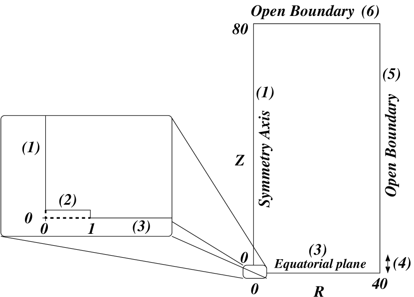
Figure 1: Schematic representation of the computational domain. The bottom left corner, containing the origin $(R,Z)=(0,0)$, is treated as an internal boundary region in order to avoid the gravitational singularity. This inner boundary enables us to treat the inner radius of the accretion disk as a mass sink, where the only requirement is to have $(V_{R},V_{Z})\leq 0$. This condition avoids unphysical mass flux entering the domain there. In the region (4), we impose the accretion rate by prescribing $\rho V_{p}$, in order to mimic the effect of the outer regions of the accretion disk. See the text for details concerning each of the 6 boundary regions.

The purpose of our simulations is to model, under symmetry assumptions, a magnetized accretion disk and the jets that can be launched from this structure. Since bipolar jets are observed in the universe, we assume that the system is symmetric with respect to the equatorial plane which we label as $Z=0$. Moreover, we assume an axial symmetry making $R=0$ a symmetry axis. We use a rectangular grid spanning a physical domain of $R=[0,40]$ and $Z=[0,80]$. The grid resolution is $154\times 304$ cells, with 2 ghost cells on each side for enforcing boundary conditions. The cell widths and heights vary non-uniformly throughout the physical domain, as both a radial and a vertical stretching is applied. In effect, this achieves a higher resolution locally in the disk.

The problem setup involves a Newtonian gravitational potential that has a singularity at the origin. In order to avoid this problem without modifying the gravity potential, we cut out several cells in the bottom left corner of the grid from the computational domain. This effectively introduces an internal boundary region. In fact, we exploit 6 different boundary regions, indicated in Fig. 1.
i) Inner boundary (Region (2) in Fig. 1)
The inner boundary is a rectangular area excluded from the computational domain. It is taken to be 2 cells high in the $Z$-direction and 14 cells wide in the $R$-direction. This number of cells corresponds to an inner boundary which radially extends to $R=1$, the inner radius of our accretion disk $R_{i}$. In this boundary region, we employ “sink” boundary conditions: in every ghost cell, the value of each quantity is copied from the third cell row $Z_{3}$ just above the excluded domain. A restriction is imposed on the poloïdal velocity. Indeed, since we are considering an accretion disk, we do not allow any positive (outward) mass flux to exist in this region and we set the internal ghost cell values for the poloïdal velocity as

$$V_{R} = min(V_{R}^{Z_{3}},0)$$

$$V_{Z} = min(V_{Z}^{Z_{3}},0)$$ (17)

Under such a flow boundary condition, the matter that fills the zone $R<R_{i}$ and $Z>0$ can only originate from the disk itself and not from the internal sink region. This is in contrast with studies done so far trying to modelize similar structures (Matsumoto et al., 1996; Kuwabara et al., 2000; Kato et al., 2002), where a modification of the gravitational potential is necessary. Such modification would not be suitable to perform long-time integrations since the accreted matter would rebound on the boundary after some time.
ii) Inflow region (Region (4))
We describe a magnetized accretion from an outer radius $R_{e}=40$ to its inner radius. Obviously, real disks extend beyond 40 internal disk radii. In order to mimic the effect of the unmodeled outer part of the accretion disk, we impose the value of the poloïdal mass flux in the ghost cells located at $R_{e}=40$ within one disk scale height only. This disk related part of the right boundary is therefore designed as a “source” region. The imposed accretion rate in this region (4), is maintained at its initial value of the disk configuration by keeping $\rho V_{R}$ and $\rho V_{Z}$ fixed at this location. The remainder of the right boundary (region (5) in Fig. 1) is treated as an open boundary (zero gradient on all conserved quantities).
iii) Equatorial plane and polar axis (Regions (1) and (3))
These boundary areas are a combination of symmetric and antisymmetric conditions. Symmetric and antisymmetric reflections of the computed values within the computational domain correspondingly set the ghost cell values. See Table 1 for the imposed conditions on the different physical quantities.

	$\rho$	$V_{R}$	$\Omega R$	$V_{Z}$	$B_{R}$	$B_{\theta}$	$B_{Z}$
Equatorial plane	symm	symm	symm	asymm	asymm	asymm	symm
Symmetry axis	symm	asymm	asymm	symm	asymm	asymm	symm

Table 1: Boundary conditions for the physical quantities at the equatorial plane ($Z=0$) and at the symmetry axis ($R=0$).

iv) Open boundaries (Region (5) and (6))
The last boundary regions we have to consider are the upper and top right boundaries. These regions are expected to receive the expelled matter from the disk, accelerated by the action of the magnetic field combined with the disk rotation. Our approach to model non-reflecting outflow conditions is very simple: the values of physical quantities in ghost cells are copied from the nearest computational cell in the direction perpendicular to the boundary surface. We check the possible influence of these boundary regions by changing the box size and repeating the simulations.

4 Accretion-ejection simulations

In this section, we present the results of our simulations. We first discuss the time evolution towards a quasi-equilibrium state. We then analyse the accretion-ejection structure which forms self-consistently and is maintained during this simulation. The parameter set is resistivity level $\alpha_{m}=0.1$, Mach sonic number $m_{s}=0.3$ and the magnetic pressure level $\beta=1.67$.

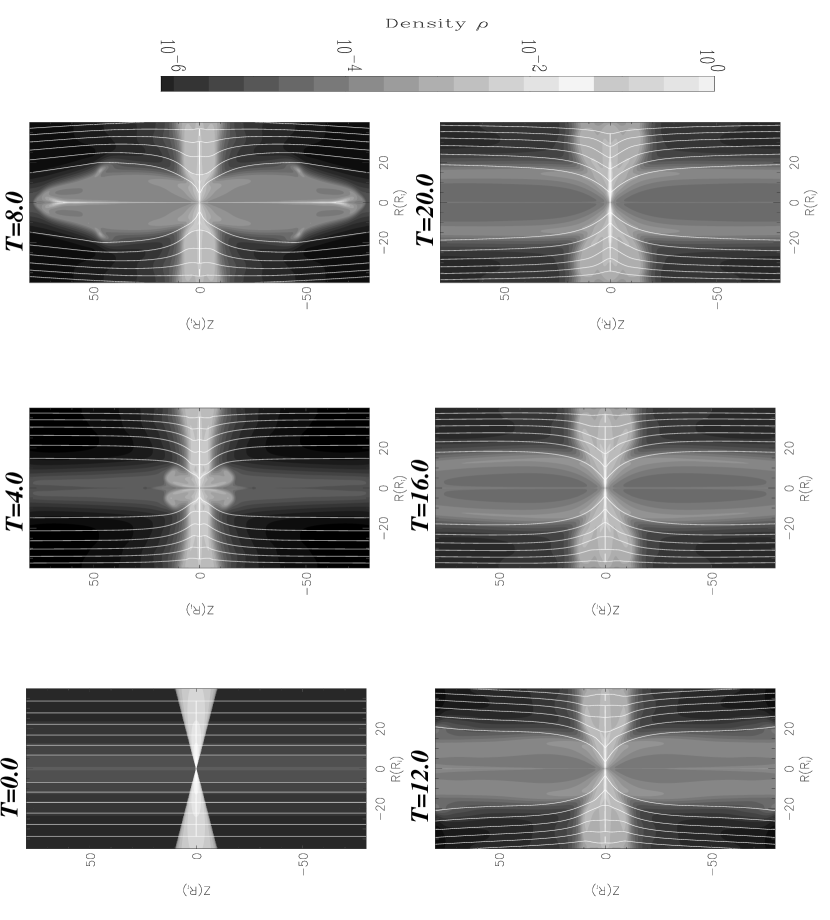
Figure 2: The dynamical evolution of a thin accretion disk threaded by an initial radially decreasing vertical magnetic field, visualized in density levels (in greyscale) and poloïdal magnetic field lines. One clearly sees a denser region being ejected from the disk along the symmetry axis, which can be identified with the jet. Collimation is already present after few dynamical time scales.

4.1 Towards steady-state

The time evolution of the structure is displayed in Fig. 2. The time unit is $1/\varepsilon\Omega_{K}$ which in this simulation represents $(2\pi\varepsilon)^{-1}=1.59$ rotation periods of matter at the inner radius. We continued this simulation until $t=25$, covering 40 periods. During this timescale, we clearly see in Fig. 2 the jet launching as a relatively dense outflow coming from the accretion disk, more precisely confined to the inner region of the accretion disk for radial distances $R\leq 20$. The collimation of this outflow is obtained within the computational domain.

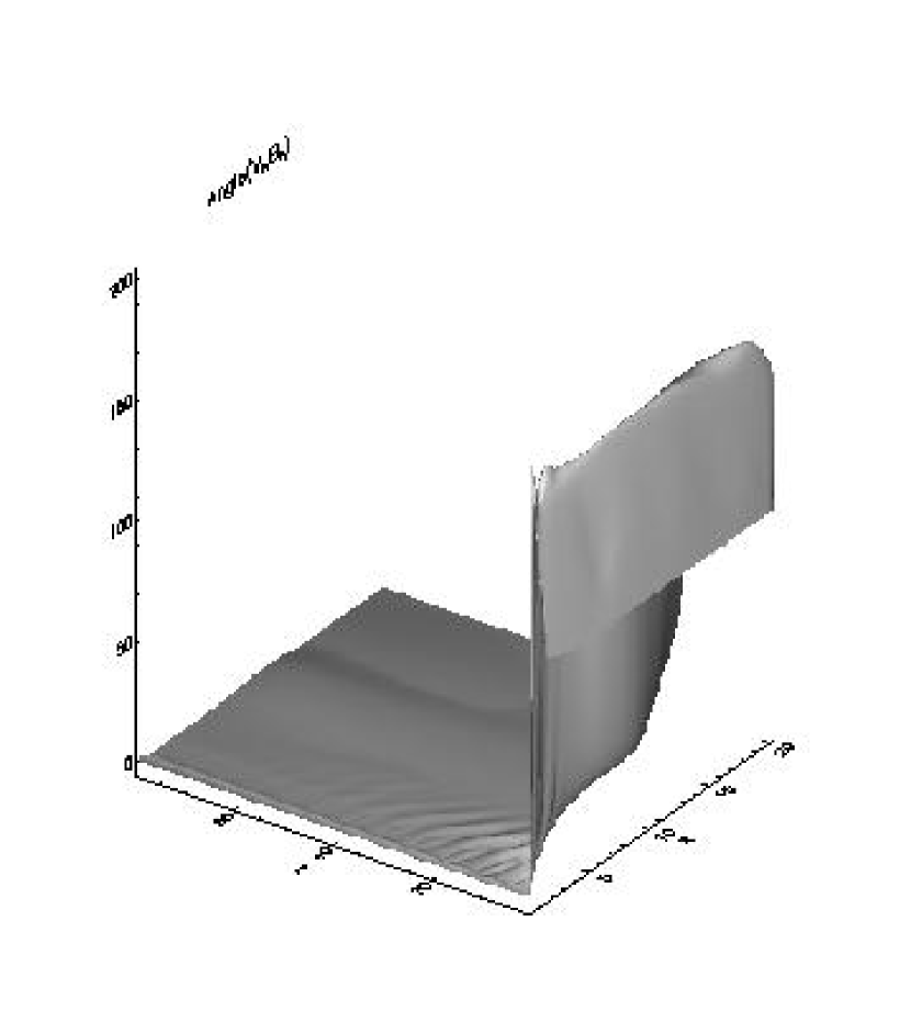
Figure 3: Measure of the angle between the poloïdal velocity and the poloïdal magnetic field within the accretion disk-jet region ($R\leq 20$) at $t=19$. In the accretion disk, the two vectors are perpendicular because the magnetic field is almost vertical and the accretion motion is radial. Moving upwards in the accretion disk, the field is bent away from the symmetry axis and a growth of $B_{R}$ is occuring. Hence, the angle increases. Above the disk, where the resistivity is vanishing, the two vectors tend to become parallel. In the jet region ($R\leq 20$ and $Z\geq 20$), the angle between $\mbox{\bf v}_{p}$ and $\mbox{\bf B}_{p}$ is everywhere smaller than $3.5^{\circ}$, so that we effectively obtain a near-perfect ideal MHD stationary jet.

To check whether the simulation is evolving towards a stationary state, we look at a quantity that would be equal to zero in a perfect ideal MHD stationary state. From the ideal MHD induction equation in an axisymmetric, stationary framework, one can deduce that the poloïdal velocity and the poloïdal magnetic surfaces have to be parallel. In Fig. 3, we display the angle between the two vectors in the launching area of the jet at $t=19$. It can be seen that above the accretion disk, this angle never exceeds $3.5^{\circ}$. This near-perfect alignment is present from times $t>17$ and is characteristic of a structure tending to a stationary configuration. Nevertheless, even at this stage, the structure is still slowly evolving in time.

Figure 4: Time evolution of the ejection rate of the structure $\dot{M}_{j}$. After the jet is launched, the ejection rate slowly decreases and then reaches a plateau. This indicates that the ejection mechanism is robust once the jet is formed. The typical amount of matter ejected from the accretion disk is roughly $\dot{M}_{j}/\dot{M}_{ae}\sim 15\%$ in this phase.

Another way to determine if the obtained emission of matter can be qualified as a robust mechanism, is by measuring the ejection rate of matter from the disk. To that end, we measure the mass flux through the surface of the disk, namely the surface where the radial velocity is vanishing. Since we impose the external accretion rate in the disk by means of our ‘source’ boundary condition (see previous paragraph), we can then obtain the ratio of the ejection rate $\dot{M}_{j}$ to the external accretion rate $\dot{M}_{ae}$. This ratio evolves in time as shown in Fig. 4. This plot shows two to three distinct phases. The first one marks the beginning of the jet launching from the disk where the ejection rate is increasing. The second phase corresponds to a relaxation of the system. Finally, the ejection rate reaches a ‘plateau’ at the end of our simulation, from about 25 rotation periods onwards. This plateau indicates that the ejection mechanism is robust and jet material is constantly launched from the disk. We did not perform a simulation to even larger integration times since these simulations are very time-consuming.

In the next subsection, we give a detailed description of a snapshot at $t=19$ of our simulation where the system has settled on a near-stationary state. This snapshot is shown in Fig. 5 where the density is displayed by greyscales, the poloïdal magnetic field lines by solid lines. Also indicated are the Alfvén ($V_{A,p}$) and fast-magnetosonic ($V_{F}$) surfaces, as represented by dotted-dashed lines. The considered velocities are defined as

$$V_{A,p}^{2}=\frac{B^{2}_{p}}{\rho}\ ;\ V_{F}^{2}=\frac{1}{2}\left\{C_{S}^{2}+V_{A}^{2}+\sqrt{(C_{S}^{2}+V_{A}^{2})^{2}-4C_{S}^{2}V_{A,p}^{2}}\right\}$$ (18)

where $V_{A}$ is the total Alfvén speed $V^{2}_{A}=(B_{p}^{2}+B^{2}_{\theta})/\rho$. We can see in this snapshot that most of the matter of the jet has been accelerated to super-fast flow speeds at the top of the computational domain. The collimation is almost complete at the top of the simulation box. Note also the distinct hollow jet structure, with the fastest moving material situated in a dense cylindrical shell at a radius $R\simeq 13$.

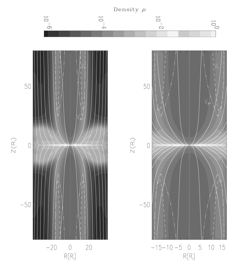
Figure 5: Snapshot of the accretion-ejection structure at $t=19$. On the left the complete computational domain is represented by setting density levels using greyscales while poloïdal magnetic field lines and critical surfaces are displayed in solid and dot-dashed lines, respectively. The right panel is a zoom of the jet launching region ($R\leq 20$).

4.2 Accretion-ejection mechanism

Figure 6: Vertical profiles of several quantities at a given radius $R=4.3$ and at $t=19$. From left to right, top to bottom: total vertical force balance, vertical component of the Lorentz force, vertical gravity component, vertical pressure gradient force, magnetic torque, angle between the poloidal velocity and the vertical, both poloidal flow components, and the density structure. On the corresponding streamlines plot shown in Fig. 7, two regimes are occuring: the first one shows streamlines reaching the inner radius in a pure accretion motion while the second one are streamlines which start to accrete but then turn back into an ejection motion. This can be explained by looking at the vertical cuts shown: the toroïdal component of the magnetic force $({\bf J}\times\mbox{\bf B})_{\theta}$ is negative inside the disk ($Z\leq 1$) and changes its sign near the disk surface. A poloïdal acceleration takes place once the sign reversal is achieved as we can see in $V_{R}$ and $V_{Z}$. These two components of poloïdal velocity stop decreasing as soon as $({\bf J}\times\mbox{\bf B})_{\theta}$ turns positive.

Figure 7: Poloïdal streamlines of the accretion-ejection structure at t=19. Two regimes can be distinguished: the first one shows streamlines reaching the inner radius in a pure accretion motion while the second one contains streamlines which start to accrete but then turn into an ejection motion. This can be explained by Fig. 6 which displays the accretion-ejection mechanism. 

In this subsection, we give a complete description of the accretion-ejection mechanism that forms spontaneously in our simulation. The mechanism is driven by the magnetic field which plays a double role. Its first role is to brake the matter in the disk and transfer angular momentum of matter to allow accretion. The magnetic torque (toroïdal component of the magnetic force ${\bf J}\times\mbox{\bf B}$) must therefore be negative in the disk. The second role of the magnetic field is to accelerate matter in the jet by providing a positive projected magnetic force along the streamlines. Such a positive projected force component is achieved if the magnetic torque changes its sign. Indeed, it is obvious that

$$({\bf J}\times\mbox{\bf B}).\mbox{\bf B}_{p}=-({\bf J}\times\mbox{\bf B}).\mbox{\bf B}_{\theta}.$$ (19)

Hence, if we assume that the poloïdal streamline is almost (or completely, in a stationary framework) parallel to the poloïdal magnetic field line, we have in the jet $\mbox{\bf v}_{p}\sim\alpha\mbox{\bf B}_{p}$. Since $B_{\theta}$ is negative, the magnetic torque must be positive in the jet for accelerating matter upwards along the magnetic field direction. A positive torque spins up jet material, and this azimuthal acceleration of the plasma increases the angular momentum of matter which leads to a dominant centrifugal force that will tend to widen the magnetic surfaces. Note that ideal MHD reasoning makes sense since the resistivity is equal to zero in the jet region.

In Fig. 6 and Fig. 7, the entire mechanism is well illustrated by showing both the streamlines of the flow in the jet launching region and several characteristic quantities along a vertical cut at a fixed radial distance of $R=4.3$. The magnetic torque ${\bf J}_{p}\times\mbox{\bf B}_{p}$ is seen to reverse its sign at about $Z=1$ and provokes a reversal of the poloïdal velocity vector. The accretion-ejection needs one more condition to work. Indeed the change of sign of the magnetic torque is a necessary condition in order to ensure that the jet will receive energy for accelerating the matter via a MHD Poynting flux. But another necessary condition is that the accretion disk must provide mass for the jet. The mass flux, and more precisely a vertical mass flux can only be achieved by a vertical force balance in the accretion disk which becomes positive (upwards) at the disk surface. At the same time, the vertical equilibrium in the interior of the accretion disk must be such that the total vertical force is negative and thereby keeps the main part of the plasma inside the accretion disk. This delicate force balance ensures that only a small fraction of the accretion disk matter escapes. If we look at Fig. 6, we see that the vertical equilibrium configuration is occuring in precisely the manner mentioned here. Plotted are all vertical forces acting on the disk, so we can identify which ones pinch the disk and which ones lift the matter up. The density profile of our accretion disk (dense near the equatorial plane and decreasing vertically) leads to a positive thermal pressure gradient that will lift the matter. On the contrary, the gravitational force pinches the disk as well as the magnetic pressure. Indeed, due to the shape of the magnetic surfaces, a growth of the radial and azimuthal component of the magnetic field occurs. This bipolar configuration leads automatically to a magnetic pinching of the accretion disk. As seen in Fig. 6 the main competition in the vertical balance is between thermal and magnetic pressure gradients, revealing that the thermal pressure must not be smaller that the magnetic one. Moreover if the magnetic pressure (i.e. magnetic field) is too small, the first condition mentioned at the beginning of this paragraph will not be fulfilled. The best configuration for emitting a fast jet of matter from an accretion disk seems then to be an accretion disk in equipartition between thermal pressure and magnetic pressure, as already noticed by Ferreira & Pelletier (1995).

From an energetic point of view, the accretion-ejection mechanism decribes the transfer of the angular momentum of the disk into the jet. Indeed, the toroïdal component of the momentum equation Eq. (3) expresses angular momentum conservation as

$$\frac{\partial\rho V_{\theta}R}{\partial t}+{\bf\nabla}\cdot\left(\rho V_{\theta}R{\bf V}_{p}-RB_{\theta}\mbox{\bf B}_{p}\right)=0\ .$$ (20)

The action of the magnetic field provides a way to extract the angular momentum of disk matter and thus enable accretion inside the disk. At the opposite, in the jet, the angular momentum stored in the magnetic field (via the generation of a toroïdal component $B_{\theta}$), can be used to accelerate matter in order to power a magneto-centrifugal jet. On Fig. 8, we display both a vertical cut and a full map of the total angular momentum flux ${\bf F}_{AM}=\rho V_{\theta}R{\bf V}_{p}-RB_{\theta}\mbox{\bf B}_{p}$. The left panels represent the matter and magnetic contributions to this flux in the radial and vertical directions. The dominant patterns are first, the storing of angular momentum by the generation of $RB_{\theta}\mbox{\bf B}_{p}$ in the disk and secondly an increase of the specific angular momentum of matter in the jet due to a magneto-centrifugal acceleration. On the right panel, the orientation of ${\bf F}_{AM}$ is displayed and we can see that the infalling radial flux in the disk is transferred to the jet along the magnetic surfaces. Note that the acceleration of matter decreases as soon as the angular momentum stored in the magnetic field reaches zero.

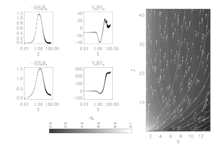
Figure 8: Left: magnetic and matter angular momentum contributions to the total angular momentum flux. Right: vector map of the total angular momentum flux ${\bf F}_{AM}=\rho V_{\theta}R{\bf V}_{p}-RB_{\theta}\mbox{\bf B}_{p}$ (arrows), poloïdal magnetic surfaces (solid lines) and amplitude of toroïdal magnetic field (greyscale). The left panels represent the different contributions to the total angular momentum flux in the radial and vertical directions. Note the extraction of angular momentum by the generation of $RB_{\theta}\mbox{\bf B}_{p}$ in the disk and secondly an increase of the specific angular momentum of jet matter due to a magneto-centrifugal acceleration. On the right panel, we can see that the infalling radial flux is evacuated in the jet along the magnetic surfaces and that the turning point occurs where $B_{\theta}$ reaches its maximum value, namely near the disk surface.

Figure 9: Radial cut of the jet structure representing radial forces acting on the plasma at $Z=40$. Two classes of forces are acting on the plasma: the ones that try to widen the flow and those that try to collimate. The first class is composed of the centrifugal force and the total pressure, while the other one contains gravity and the magnetic tension due to the presence of a toroïdal magnetic field. This figure illustrates that only the presence of $B_{\theta}$ is able to counteract other forces in the jet region where gravity is almost negligible. Note that we do not involve any external mechanism to ensure the collimation of the flow.

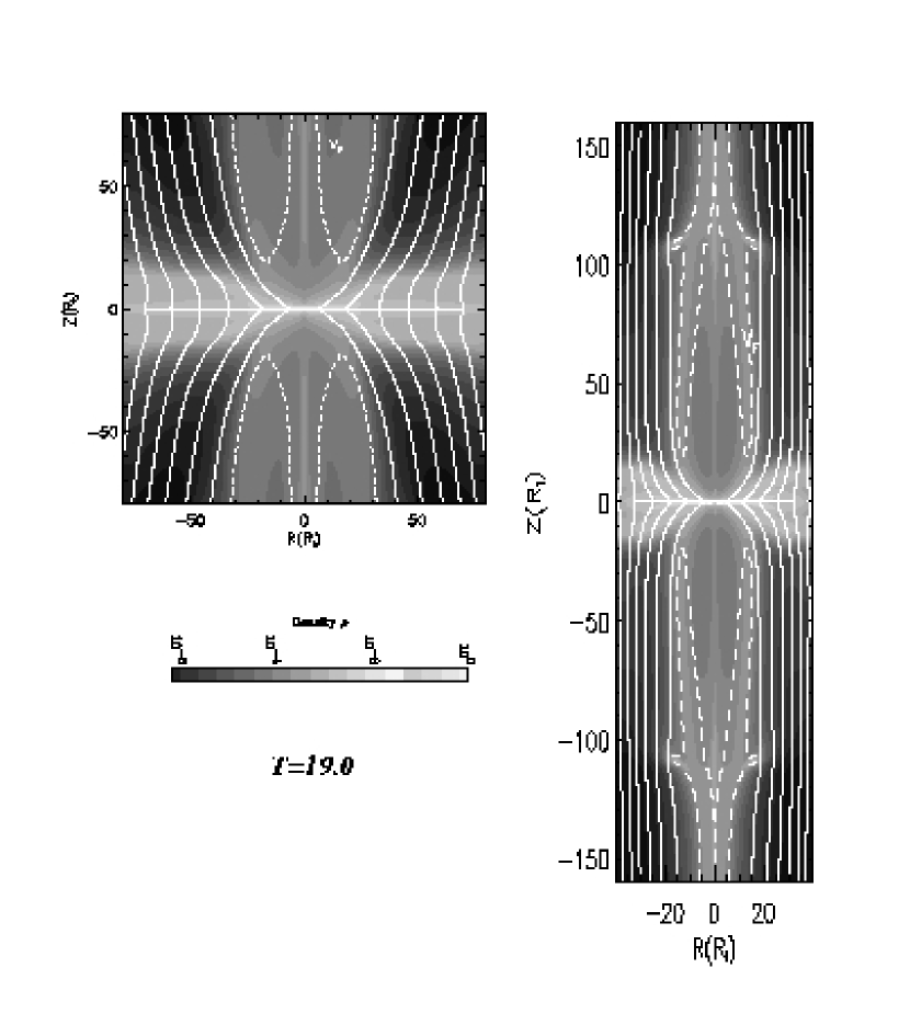
Figure 10: Snapshots of two equivalent MHD simulations on extended domains using the same initial conditions as the reference simulation of Fig. 2 and at the same physical time $t=19$, to be compared with Fig. 5. The influence of the boundary conditions is marginal, as all simulations reach very similar super-fast collimated outflow launched from the inner disk region alone.

It is important to note that after the acceleration has taken place, the collimation of the flow is quite good since the maximal value of the angle between the vertical direction and the velocity in the highest regions of our box is never bigger than $1.5^{\circ}$ (see Fig. 6). The collimation of the flow is due to a mechanism internal to the jet structure being formed. This is demonstrated in Fig. 9, showing all the radial forces existing in the jet at a horizontal cut at $Z=40$. These are the centrigugal force, the thermal and magnetic pressure gradients, gravity and magnetic tension. Clearly, the force assuring the collimation of the flow is the magnetic tension or “hoop” stress ($B^{2}_{\theta}/R$). Contrary to all other forces (except gravity which can be neglected so far from the disk), it is the only force that is always directed towards the symmetry axis. Looking at the sum of all forces in the radial direction indicates that the plasma is not yet in a full stationary state but has come quite close to achieving a radial equilibrium balance. However, we can not exclude the possibility that eventually some hydrodynamic or magnetic instabilities develop somewhere in the structure (Kim & Ostriker, 2000). This should be verified by performing the same simulation in three dimensions.

4.3 Influence of open boundaries

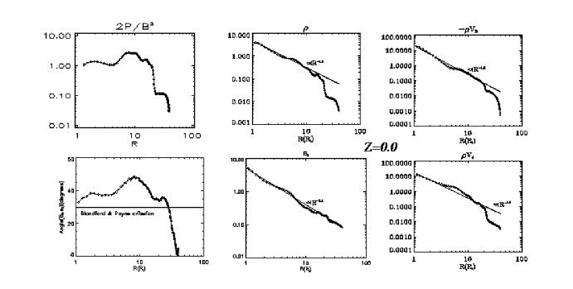
Figure 11: Ratio of thermal pressure to magnetic pressure, radial profiles of physical quantities ($\rho,-\rho V_{R},B_{z},\rho V_{\theta}$) along the equatorial plane ($Z=0$), and angle between $\mbox{\bf B}_{p}$ and ${\bf e}_{z}$ at the disk surface (where the radial velocity is vanishing). The $\beta$ ratio explains why the inner part of the disk launches a jet while the outer part does not: only the inner part is in equipartition, a necessary condition ensuring that the vertical disk equilibrium can supply matter for the jet formation. Moreover, as shown by the bottom left plot, only the inner region has a suitable magnetic configuration for matter acceleration in the jet. The behaviour of quantities along the equatorial plane is close to radial power-law with indices modified in comparison to the initial conditions. The power-law indices are in relatively good agreement with self-similar MAES models from Casse & Ferreira (2000a).

Modeling a magnetized, resistive accretion disk and its associated ideal MHD trans-Alfvénic jet numerically requires to control the effect of, in particular, the open boundaries bordering the computational domain. Indeed, as already shown by Ustyugova et al. (1995), if not modeled appropriately, they can influence the dynamics of the system, e.g. by unwanted reflections. To check the potential effect of our boundary conditions on the simulated flows, we repeated all our simulations using different sizes for the computational domain. While our reference simulation uses a $[0-40]\times[0-80]$ rectangular box, we performed the same calculation with rectangular boxes covering $[0-80]\times[0-80]$ and $[0-40]\times[0-160]$, with resolutions of $204\times 104$ and $104\times 404$, respectively. The jet launching was found to occur in every simulation and, most importantly, remains restricted to roughly the same part of the physical domain (within $1-20$ radius range), as shown in Fig. 10. Nevertheless, small differences do exist between these three simulations. The radial extension of the computational domain seems to have an influence on the exact radial size of the jet launching region. This indicates a marginal influence from the open boundary at the right side of the box. Repeating the simulations while gradually extending the radial box size, a systematic larger jet launching radial range is obtained. The effect is probably also due to differences in effective local resolution, but can be observed by comparing Fig. 5 with the left panel of Fig. 10. The simulation which doubled the vertical extent (right panel of Fig. 10) is in very good agreement with the reference solution. Hence the top open boundary has no influence on the obtained dynamics.

4.4 Accretion disk structure

The radial accretion disk structure largely determines its stability to MHD perturbations (Keppens et al., 2002). Up to the present work, the only model able to include both a resistive accretion disk and a super-Alfvénic jet without neglecting any dynamical quantities in the equilibrium of the structure was a self-similar model used by Ferreira (1997) and Casse & Ferreira (2000a). This model assumed that, to simplify the analysis, all physical quantities $A$ appearing in the set of MHD equations can be written as

$$A(R,Z)=A_{e}\left(\frac{R}{R_{e}}\right)^{\alpha_{A}}f_{A}\left(\frac{Z}{R}\right),$$ (21)

where $\alpha_{A}$ is a coefficient imposed by the smooth crossing of the Alfvénic surface. Hence, each quantity was represented by a power-law dependence on radius $R$ and a separate polar angle variation $f_{A}$. Since the initial conditions of our simulation are derived from a self-similar configuration, it is worthwhile to confront this with the obtained final radial structure of our accretion disk. In Fig. 11, we display the radial profiles of several physical quantities at the disk midplane $Z=0$. We clearly see two different regions. The first one which reaches up to $R\leq 20$ corresponds to the jet launching region and features a radial behaviour of all quantities close to power-law. As compared to their $t=0$ values, these indices are modified. Indeed, in our initial conditions, the indices for density $\rho$, momentum $\rho\mbox{\bf v}$ and magnetic field $B_{z}$ were $-3/2,-2$ and $-5/4$. These initial values correspond, in the case of self-similar MAES, to a magnetized accretion disk where no ejection occurs. In the final disk structure shown in Fig. 11, the indices have become $\alpha_{\rho}>-3/2$, $\alpha_{\rho v}>-2$ and $\alpha_{B}>-5/4$. Such a systematic modification to larger values is consistent with self-similar MAES models that allow ejection. Indeed, the presence of a jet makes the effective local accretion rate a decreasing function for smaller radii and this modifies the power-law radial indices of the quantities. Our simulation shows that the final disk structure displays a second region where the quantities, except for the magnetic field, do not have a clear power-law behaviour. This explains why this outer disk region does not launch a jet. Indeed, the parameter $\beta=2P/B^{2}$ which was set to a constant value of $1.67$ at $t=0$, has adjusted to a very low value outside the jet launching region. As explained before, this prevents the vertical force balance in the disk to allow matter escaping from the disk and providing a mass source for the jet. Moreover, the angle of the poloïdal magnetic field with respect to the vertical direction measured at the disk surface (where resistivity is vanishing), is suitable for jet launching only in the inner region. Indeed Blandford & Payne (1982) has shown that any cold steady-state jet must have, bent poloïdal magnetic surfaces with an angle larger than thirty degrees, in order to achieve an acceleration by the action of the magnetic field. In Fig. 11, on the left bottom panel, we show the angle between the magnetic surface and the vertical direction measured at the disk surface (typically where $V_{R}$ changes its sign). It is clear from this figure that only the inner part of the structure is able to launch a jet. Nevertheless, the suitable bending of the magnetic surfaces is ranging from $R=1$ to $R\simeq 30$ in contrast with the effective jet launching region that ranges from $1$ to $\sim 15$. This is a good illustration that both jet launching conditions must be fulfilled: in the region between $16$ to $30$, the vertical balance of the disk is not suitable for a positive mass flux).

5 Concluding remarks and outlook

We present in this work the first MHD simulations of a magnetized, resistive accretion disk launching an ideal trans-Alfvénic jet. The simulations are performed in a 2.5 dimensional, time-dependent and polytropic framework. Our MHD simulations involve a magnetic resistivity that is only triggered within the accretion disk. The shape of the resistivity coefficient is derived from Shakura & Sunyaev (1973) since we express it as $\eta=\alpha_{m}V_{A}|_{Z=0}H\exp(-2Z^{2}/H^{2})$ where $V_{A}$ stands for Alfvén velocity, $H$ disk scale-height and $\alpha_{m}$ is a dimensionless parameter controlling the amplitude of the resistivity, smaller than unity). The temporal behaviour of our simulations display the launching of an outflow that, while propagating, becomes collimated. Note that the jet reaches super-fastmagnetosonic velocities within our computational domain. The long term robustness of the structure is demonstrated by several means. In particular, we check the angle between poloïdal velocity and poloïdal magnetic field (which is zero in a pure ideal MHD stationary configuration) and show that, after the outflow has been launched, this angle reaches maximum values in the jet typically smaller than three degrees. Moreover, the ejection rate (mass flux through the disk surface) of the disk, once initiated, remains near-constant over several tens of the accretion disk dynamical timescale. These diagnostics characterize a robust system that has reached a quasi-stationary state.

We also present in this paper, by a detailed scrutiny of one snapshot of our simulation in the near-stationary phase, a complete illustration of the so-called ‘accretion-ejection’ mechanism that is responsible for the jet launching. The key point of this model is that disk resistivity enables the structure to reach a near-static equilibrium where accreted matter inside the disk can pass through the poloïdal magnetic surface. Such resistivity would mimic the effects of turbulence occuring inside the disk, provoked by MHD instabilities affecting equipartion accretion disks (Keppens et al., 2002). Moreover, we confirm by self-consistent numerical simulations that the two necessary conditions to achieve such a jet creation are (1) a vertical disk equilibrium which allows some disk matter streamlines to reach the disk surface (typically an equipartition disk with $B^{2}/P\sim 1$, Ferreira & Pelletier (1995)) and (2) a turbulence configuration that obeys a simple relation Eq. (16) already presented in Casse & Ferreira (2000a). In our simulations, since we do not take viscosity into account, the angular momentum of disk matter is transferred by the action of a magnetic torque acting on the disk plasma. We highlight the fact that the sign reversal of the magnetic torque at the disk surface, obtained in self-similar analytic models if the turbulence follows the relation 16, is the core of the magneto-centrifugal effect responsible for jet acceleration. By displaying the radial force balance in the jet, we illustrate the role of the toroïdal component of the magnetic field which collimates the outflow by means of magnetic tension (also called “hoop” stress, see Heyvaerts & Norman (1989)).

Forthcoming work will focus on two major points that were not taken into account here. Indeed, future work should be devoted to the implementation of a viscous torque inside the disk. This approach will validate the knowledge on complex angular momentum transport by both magnetic and viscous torques (Casse & Ferreira, 2000a; Ogilvie & Livio, 2001) combined with jet launching. The second point is the relevance of the energy equation in this kind of system. Specifically, it has been demonstrated in a self-similar framework that the existence of a hot corona located at the disk surface is relevant to the astrophysical outflow (Casse & Ferreira, 2000b; Garcia et al., 2001). So the use of a full energy equation is desirable. The simulations presented here consider a time-dependent resistivity (through the value of the Alfvén speed in the disk). This could be of great interest for scenarios looking at time-dependent disk models launching jets, in particular for microquasars (Tagger & Pellat, 1999; Nayakshin et al., 2000). Indeed, a suitable prescription of the transport coefficients could be able to produce structures where a periodic jet launching occurs.

References

- Balbus & Hawley (1998) Balbus, S.A. & Hawley, J.F. 1998, Rev. of Modern Physics, 70, 1
- Blandford (1976) Blandford, R.D. 1976, MNRAS, 176, 465
- Blandford & Payne (1982) Blandford, R.D. & Payne, D.G. 1982, MNRAS, 199, 883
- Brackbill & Barnes (1980) Brackbill, J.U., Barnes, D.C. 1980, J. Comp. Phys., 35, 426
- Cabrit et al. (1990) Cabrit, S., Edwards, S., Strom, S.E. & Strom, K.M. 1990, ApJ, 354, 687
- Casse & Ferreira (2000a) Casse F. & Ferreira J., 2000a A&A, 353, 1115
- Casse & Ferreira (2000b) Casse F. & Ferreira J., 2000b A&A, 361, 1178
- Curtis (1918) Curtis, H.D. 1918, Lick Observatory publications
- Eikenberry et al. (1998) Eikenberry, S.S., Matthews, K., Morgan, E.H. et al. 1998, ApJ, 494, L61
- Ferreira & Pelletier (1993) Ferreira J. & Pelletier G., 1993 A&A, 276, 625
- Ferreira & Pelletier (1995) Ferreira J. & Pelletier G., 1995 A&A, 295, 807
- Ferreira (1997) Ferreira J. 1997 A&A, 319, 340
- Frank et al. (1985) Frank, J., King, A.R. & Raine, D.J., “Accretion power in Astrophysics” 1985, Cambridge University Press
- Garcia et al. (2001) Garcia P.J.V., Cabrit S., Ferreira J., Binette L. 2001, A&A, 377, 609
- Hartigan et al. (1995) Hartigan, P., Edwards, S. & Ghandour, L. 1995, ApJ, 452, 736
- Heyvaerts & Norman (1989) Heyvaerts, J. & Norman C. 1989, ApJ, 347, 1055
- Kato et al. (2002) Kato, S., Kudoh, T., Shibata, K. 2002, ApJ, 565, 1035
- Keppens et al. (2002) Keppens, R., Casse, F. & Goedbloed, J.P. 2002, ApJ, 569, L121
- Kim & Ostriker (2000) Kim, W.T. & Ostriker, E.C. 2000, ApJ, 540, 372
- Krasnopolski et al. (1999) Krasnopolski, R., Li, Z.Y. & Blandford, R.D. 1999, ApJ, 526, 631
- Kuwabara et al. (2000) Kuwabara, T., Shibata, K., Kudoh, T. & Matsumoto, R. 2000, PASJ, 52, 1109
- Li (1995) Li, Z.Y. 1995, ApJ, 444,848
- Li (1996) Li, Z.Y. 1996, ApJ, 465, 855
- Livio (1997) Livio, M. 1997, in IAU Colloquium 163. ASP Conference Series; Vol. 121; eds. D. T. Wickramasinghe; G. V. Bicknell; and L. Ferrario (1997), p.845
- Lovelace (1976) Lovelace, R.V.E. 1976, Nature, 262, 649
- Matsumoto et al. (1996) Matsumoto, R., Ushida, S., Hirose, K. et al. 1996, ApJ, 461, 115
- Mirabel & Rodríguez (1999) Mirabel, I.F. & Rodrìguez, L.F. 1999, ARA&A, 37, 409
- Mirabel et al. (1998) Mirabel, I.F., Dhawan, V., Chaty, S., et al. 1998, A&A, 330, L9
- Mouschovias (1976) Mouschovias, T.C. 1976, ApJ, 206, 753
- Nayakshin et al. (2000) Nayakshin, S., Rappaport, S. & Melia, F. 2000, ApJ, 535, 798
- Ogilvie & Livio (2001) Ogilvie, G.I. & Livio, M. 2001, ApJ, 553, 158
- Ouyed & Pudritz (1997) Ouyed, R. & Pudritz, R. 1997, ApJ, 482, 712
- Rekowski et al. (2000) Rekowski, M.V., Rüdiger, G. & Elstner, D. 2000, A&A, 353, 813
- Sauty et al. (2002) Sauty, C., Trussoni, E. & Tsinganos, K. 2002, A&A, in press
- Serjeant et al. (1998) Serjeant, S., Rawlings, S., Lacy, M. et al. 1998, MNRAS, 294, 494
- Shakura & Sunyaev (1973) Shakura, N.I., Sunyaev, R.A. 1973, A&A, 24, 337
- Tagger & Pellat (1999) Tagger, M., Pellat, R. 1999, A&A, 349, 1003
- Tóth (1996) Tóth, G. 1996, Astrophys. Lett., 34, 245
- Tóth & Odstrčil (1996) Tóth, G. & Odstrčil, D. 1996, J. Comp. Phys., 128, 82
- Tóth (2000) Tóth, G. 2000, J. Comp. Phys., 161, 605
- Ushida & Shibata (1985) Ushida, Y. & Shibata, K. 1985, PASJ37, 515
- Ustyugova et al. (1995) Ustyugova, G.V., Koldoba, A.V., Romanova, M.N., Chetchetkin, V.M. & Lovelace, R.V.E. 1995, ApJ, 439, L39
- Vermeulen & Cohen (1994) Vermeulen, R.C. & Cohen, M.H. 1994, ApJ, 430, 467
- Wardle & Königl (1993) Wardle, M. & Königl, A. 1993, ApJ, 410, 218