$\dagger$  Current address: Department of Astronomy University of Maryland College Park, MD 20742 farnham@astro.umd.edu

Abstract

We present imaging and spectroscopic data on comet 19P/Borrelly that were obtained around the time of the Deep Space 1 encounter and in subsequent months. In the four months after perihelion, the comet showed a strong primary (sunward) jet that is aligned with the nucleus’ spin axis. A weaker secondary jet on the opposite hemisphere appeared to became active around the end of 2001, when the primary jet was shutting down. We investigated the gas and dust distributions in the coma, which exhibited strong asymmetries in the sunward/anti-sunward direction. A comparison of the CN and C₂ distributions from 2001 and 1994 (during times when the viewing geometry was almost identical) shows a remarkable similarity, indicating that the comet’s activity is essentially repeatable from one apparition to the next. We also measured the dust reflectivities as a function of wavelength and position in the coma, and, though the dust was very red overall, we again found variations with respect to the solar direction. We used the primary jet’s appearance on several dates to determine the orientation of the rotation pole to be $\alpha=214^{\circ}$, $\delta=-5^{\circ}$. We compared this result to published images from 1994 to conclude that the nucleus is near a state of simple rotation. However, data from the 1911, 1918 and 1925 apparitions indicate that the pole might have shifted by 5-10^∘ since the comet was discovered. Using our pole position and the published nongravitational acceleration terms, we computed a mass of the nucleus of $3.3\times 10^{16}$ g and a bulk density of 0.49 g cm^-3 (with a range of $0.29<\rho<0.83$ g cm^-3). This result is the least model-dependent comet density known to date.

Keywords: Comets; Rotational Dynamics; Spectroscopy; Imaging; Comet, Dynamics

1 Introduction

On 22 September 2001 UT, NASA’s Deep Space 1 (DS1) spacecraft made a close flyby of the nucleus of comet 19P/Borrelly, obtaining high-resolution images, infrared spectra and particles and fields measurements within about 12 hours of closest approach (Soderblom et al. 2002). The images that were obtained offer an unprecedented look at the nucleus of this comet and promise to reveal many details about the innermost region of the coma as well as the topology and albedo of the nucleus. However, due to the rapid velocity and short duration of the encounter, additional information is needed to provide a more global interpretation of the spacecraft measurements and how they relate to observations of the entire coma.

In support of this mission, we utilized the 2.1-m and 2.7-m telescopes of McDonald Observatory to observe comet Borrelly around the time of the DS1 encounter and in subsequent months. We obtained both moderate-resolution spectroscopy and broad band imaging in R and V filters. In this paper we describe our observations and discuss how they were used to analyze the morphology of the coma, probe the asymmetric distributions of the gas and dust, and derive the reflectivity of the dust. We then highlight some unique inherent physical characteristics of the comet and discuss how they were used to determine the orientation of the spin axis. Finally, we present an analysis in which we used our pole determination and the comet’s nongravitational forces to constrain the mass and density of the nucleus. We also compare our results to those found from earlier apparitions (Cochran and Barker 1999) and to other observers’ results from this apparition, including the DS1 measurements.

2 Observations and Reductions

We obtained two different types of data on comet Borrelly during the 2001 apparition: moderate-resolution spectroscopy and broad-band imaging. Table I is a log of our observations and a summary of the geometric conditions.

2.1 Spectroscopy

The spectroscopic observations were obtained using the McDonald Observatory Electronic Spectrograph No. 2 (ES2) on the 2.1-m Otto Struve telescope. The detector was a TI $800\times 800$ pixel CCD with 15 $\mu$m pixels that were binned by a factor of 2 in the spatial direction. The spectrograph is a long slit instrument with a slit length of almost 200 arcsec; each binned pixel subtends 1.89 arcsec on the sky. For the observations of the comet and solar analogue stars, the slit was 2.1 arcsec wide. The slit was widened to 12 arcsec for spectrophotometric standard stars in order to ensure no loss of light. The nominal 2-pixel resolution was 6.5Å. The spectra covered the bandpass from 3043–5680Å in September and 3220–5872Å in November.

The reduction of the data proceeded in a standard manner with removal of the bias using a masked region of the chip and of the pixel-to-pixel sensitivity variation using observations of an incandescent (flat field) lamp. Wavelength calibrations were performed with spectra of an argon lamp observed at the same position as the objects. Flux calibration was accomplished with observations of spectrophotometric standards (Stone 1977).

In normal operation, the slit is oriented east/west. However, this orientation can be altered by rotating the instrument on the telescope. The position angle (PA) of the slit on the sky for the observations is noted in Table I. Guiding was accomplished by imaging the slit with a CCD guide camera so that we were guiding directly on the cometary image. Care was taken to observe the argon lamp at each slit orientation to map any possible motions of the spectrum on the detector produced by rotating the instrument.

The spectrum of any comet consists of a combination of molecular emissions, generally from resonance fluorescence, superimposed on a solar spectrum reflected from the dust. In order to study the distribution of the gas in the coma, we removed the underlying continuum and then integrated across the emission band wavelengths. We used observations of solar analogue stars obtained during the same observing runs to represent the solar spectrum. Complete details of our analysis procedures can be found in Cochran et al. (1992). The bandpasses for the gas and continuum can be found in Table I of that paper and the constants for conversion of the band intensities to column densities can be found in Table II of that paper.

Since the “apertures” of a slit spectrograph are very small, with most of the apertures not including the optocenter, the standard $Af\rho$ formalism of A’Hearn et al. (1984) is not very useful for studying the dust with our spectra. These problems were discussed in detail by Storrs et al. (1992). Instead of using the $Af\rho$ formalism, we studied the dust in the coma by determining the flux in the continuum regions of the spectrum without removing the solar spectrum. Some of these bandpasses are slightly contaminated by gas but the complex nature of the cometary spectrum makes observing true continuum difficult. However, with the use of a spectrograph, we can isolate continuum regions more easily than with narrow-band filters. We can also ratio the derived fluxes to the observed solar flux (from observations of the solar analogue) in the same bandpasses in order to determine the relative reflectivity of the dust.

2.2 Imaging

We obtained imaging data on a total of five observing runs at McDonald Observatory, under the geometric conditions listed in Table I. The December 2001 data were obtained with the 2.1-m Otto Struve Telescope, and data from the other four runs were obtained with the 2.7-m Harlan J. Smith telescope. In both cases, the Imaging Grism Instrument, a 5:1 focal reducer, and a TeK 1024$\times$1024 CCD (which is partly vignetted on both telescopes) were used. On the 2.7-m, this configuration produces a 7 arcmin field with 0.57 arcsec pixels. On the 2.1-m, the result is a 6 arcmin field with 0.48 arcsec pixels. During the September and November runs and on 6-7 December, the seeing was typically between 1 and 2 arcsec (FWHM); on 4 and 5 December, it was highly variable, ranging from 2.5 to 4 arcsec; during the February run, it was typically around 2.5 arcsec; and in May it was about 3 arcsec.

Processing of the CCD images followed standard procedures and was done using the CCD reduction packages in the Image Reduction and Analysis Facility (IRAF). The bias was removed in two steps, first applying the overscan region to remove the bulk value, and then subtracting a master bias frame, created by averaging many bias images, to remove the residual for each individual pixel. Flat fielding was done using twilight sky flats that were medianed together to remove stars.

Many of the images were obtained under non-photometric conditions, but for all except the May observing run, at least one night per run was of sufficient quality to provide an absolute calibration. On these nights, Landolt standards (Landolt 1992) were observed at several airmasses and in both filters so the extinction per airmass and color coefficients of the extinction could be determined, as well as the zero-point offset of the instrumental magnitudes. Using the standard star information, the comet images were converted to the standard magnitude system, and ultimately to absolute fluxes. Finally, in order to compare the inherent brightness levels of the comet between the four observing runs, the fluxes were converted to total luminosities by multiplying by $4\pi\Delta^{2}$. No calibration was done for the May data.

The December observing run presented a couple of problems that affected the quality of the data. The 2.1-m telescope does not track very well at cometary rates, and even though short exposures were used to avoid significant trailing, there are still guiding problems in some of the images. (Note that the tracking problems did not affect the spectra, because, in those observations, we guided actively on the comet image on the slit.) The two photometric nights from the December run had poor seeing, while the two nights that had decent seeing were non-photometric. To produce the best representative images from this run, we calibrated the images from 4 and 5 December using the standard star measurements (being careful to account for seeing variations during each night) and then used the total brightness of the coma to calibrate the images from 6 December. This makes the inherent assumption that the comet’s brightness is not changing on daily timescales, but a comparison of the images from 4 and 5 December supports this assumption. It is possible that a minor outburst could have occurred between December 5 and 6, but there is no morphological evidence for this.

3 Results

3.1 Appearance and Evolution of the Coma

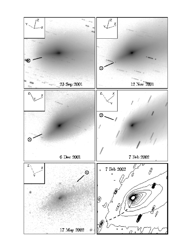
Figure 1: Farnham and Cochran

The appearance of comet Borrelly, as shown in representative images in Figure 1, provides a record of the temporal evolution of the coma during the months after perihelion. In September (during the DS1 encounter) the inner coma was dominated by a straight, narrow feature that pointed to within 7^∘ of the sunward direction as projected onto the plane of the sky. We know that this feature is not a classical anti-tail, which is produced by projection effects of the dust tail as the Earth passes through the comet’s orbit, because the Earth was 19.5^∘ above the comet’s orbital plane at the time. Therefore, it must be a jet, produced by an isolated active region on the comet’s surface, and we have designated it the “primary jet.” The width of this jet was about 35^∘ (FWHM). A dust tail was obvious in the anti-solar direction but it was noticeably fainter than the jet. Throughout the following months, the general morphology was similar, but the jet seemed to fade relative to the rest of the coma. In November, the primary jet was closely aligned with the sunward direction, but its brightness had dropped to the point that it was comparable to that of the dust tail. By December, the jet was fainter than the dust tail and was pointed at an angle about 15^∘ from the apparent sunward direction.

Measurements by Lamy et al. (1998) and Mueller and Samarasinha (2002) indicate that the comet is rotating with a period of 25–26 hours. Given the time span of our observations in September and December, we have coverage of about one-quarter of a rotation on each run, so we should expect to see evidence of rotation in our images. However, we see no indication that the coma was changing, on timescales of either hours or days. We searched for evidence of temporal variations (e.g., a change in the jet’s PA or a non-radial morphology formed by the material spiraling outward from the rotating nucleus) but found none. Even with the application of image enhancement techniques, including 1/$\rho$ removal, digital filters and unsharp masking, we could see no apparent change in the jet PA or deviations from a purely radial morphology. It is possible that the rotation axis could be oriented such that, in one of the observing runs, the jet might show little change (for example, if the axis were parallel to the plane of the sky and the jet were rotating along the line of sight). However, changes in the viewing geometry from September to December make it extremely unlikely that this could occur during all three of these observing runs. Therefore, the lack of any movement or curvature in the primary jet leads us to conclude that it must be situated close to the rotation pole of the nucleus. Samarasinha and Mueller (2002) come to this same conclusion and invoke dynamical arguments to further conclude that the nucleus must be very close to a state of principle axis rotation. We address the comet’s rotation state in more detail in Section 3.5.

By February, the comet’s appearance had changed somewhat. A well-defined, curved jet was visible, extending out from the nucleus at a position angle of $\sim 335^{\circ}$, roughly perpendicular to the projected sunward direction. Is this jet simply a different projection of the primary jet, or is it a new active region not previously seen? We can address this question using the basic geometry of the comet’s orbit. The inset panels in Figure 1 show an inertial reference frame based on the comet’s orbital plane (the X axis points in the anti-solar direction at perihelion and the Z axis is parallel to the orbital angular momentum vector). In the September, November and December images, the primary jet consistently extended in the –X direction, while the jet observed in February clearly lies in the +X direction. Because the projection effects shifted only gradually during our observations, with remarkably little change from December through May, we conclude that the feature seen in February is a secondary jet that points in the opposite direction from the primary jet. The changing relative brightnesses of the two jets suggest that seasonal effects caused the primary active region to shut down while the secondary became more active. The curvature of the secondary jet can be attributed either to the spiral effect produced by rotation of the nucleus or to the effects of radiation pressure, which is acting roughly perpendicular to the jet axis. Unfortunately, our February observations were not extensive enough to look for motion of the jet as a function of time, so we cannot differentiate between these possibilities.

The February image also shows a protrusion of the coma in the southeast direction. At first glance, this extension appears to have the same radial structure as the primary jet in the September, November and December images, suggesting that the primary jet might continue to be active. Upon further inspection, however, it is clear that the February feature is not truly radial, but appears to be a linear structure that is offset from the nucleus. To illustrate this, a contour plot is shown in Fig. 1, with a dashed line connecting the points of the protrusion for each contour level. At large cometocentric distances, the protrusion is nearly linear, but is offset so that if it were extended, it would not intersect the nucleus. Only at smaller distances, where the central coma dominates the brightness, does the dashed line curve in toward the nucleus. The fact that the protrusion does not extend radially in to the nucleus means that it is not produced by continuous activity from the primary jet in the same manner as it was from September through December. Instead, the protrusion must be composed of relatively large dust particles that were emitted from the primary jet earlier in the apparition and are only slowly being blown away from the sun by radiation pressure. Schleicher et al. (2002) observed this same protrusion in their January data and came to the same conclusion.

Finally, Fig. 1 also shows a picture from the May observing run. Even though the image quality is poor, the secondary jet can be seen at a PA of 308^∘. Again, our data set is too limited to search for changes in the jet as a function of time. Also, the signal-to-noise is too low to unambiguously follow the jet to more than about $2\times 10^{4}$ km from the nucleus, which means we can’t look for spiral structures that would provide clues to the rotation period or the location of the active region.

3.2 The Distribution of the Gas in the Coma

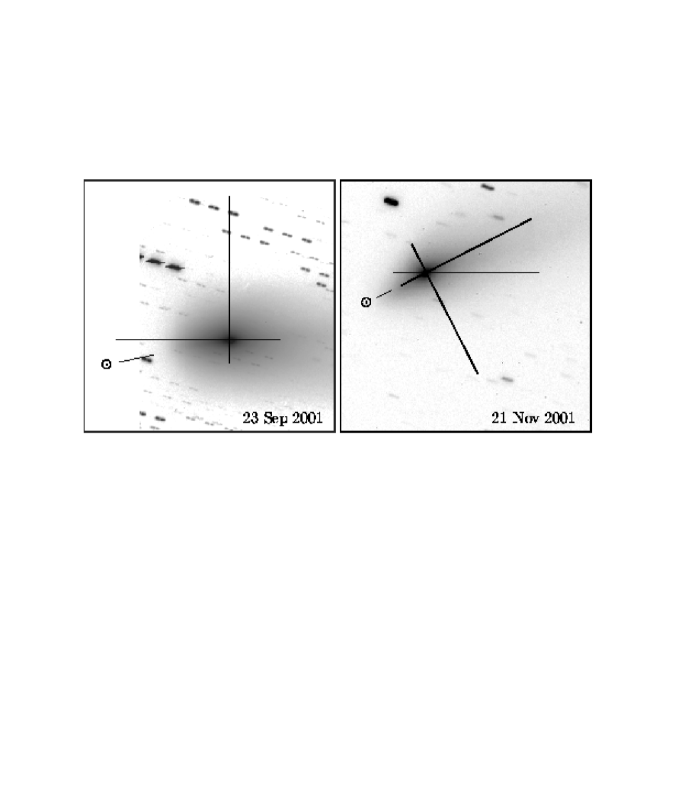
Figure 2: Farnham and Cochran

Our spectroscopic bandpass allows for the detection of CN, C₂, C₃, CH and NH and also for detection of OH in September and NH₂ in November. For each spatial pixel (1.89 arcsec) along the extent of the slit, we can measure the band intensities of the molecules and convert them to column densities. Figure 2 shows images of the comet with the positions of the slit marked on them for the observing runs for which we obtained spectra. We can then use the spectroscopic data to probe the distribution of the gas along certain vectors. Figure 3 shows the spectrum of comet Borrelly at the optocenter location and 20,000 km north of the optocenter. For comparison, another cometary spectrum obtained with a comparable instrument is shown. Note that the Borrelly optocenter spectrum shows more continuum than the off-optocenter spectrum. Compared with comet C/1996 B1 (Szczepanski), the C₂ and C₃ in Borrelly are less strong relative to the CN.

Figure 4 shows the derived column densities as a function of cometocentric distance for C₂ and CN on each night that spectra were obtained. At least two spectral images were obtained on each night, with five images obtained on 22 September. The column densities from each spectral image are denoted with a different symbol. The optocenter of the comet was always imaged on part of the slit, and the colors in the plot indicate on which side of the optocenter a column density was measured.

Several points are noteworthy from this figure. There is excellent agreement among the column densities derived from the different spectral images on each night. Indeed, one can estimate a low level of uncertainty in the measured column densities from the small spread in the data. When the slit was oriented along the the Sun/anti-Sun line (parallel direction), the gas shows a highly asymmetric distribution, which is much larger than the uncertainties in the data. However, when the slit was aligned perpendicular to this line (perpendicular direction), the gas distribution seems quite symmetric.

We have fit a Haser model (Haser 1957) to the data from 23 September and the distribution perpendicular to the Sun/anti-Sun direction on 21 November in order to derive the production rates, $Q$. Although these models assume spherical symmetry, which is clearly not in evidence for Borrelly, we are simply using the Haser fits as a comparison tool for visualizing the differences in the different distributions. We adopted the Haser model scalelengths of Randall et al. (1992), which were also adopted by A’Hearn et al. (1995). These scalelengths are different from those we used previously (Cochran and Barker 1999), but they fit the September data better than the previous values. We adopted a constant velocity of 1 km sec^-1, so we have actually derived $Q/v$. The values of $Q/v$ were chosen for the best fit to all of the data, weighted by the signal/noise of the column densities. The derived Haser production rates are indicated in the appropriate panels of the plot and are listed in Table II.

The Haser fit to the CN data of 23 September is excellent. For C₂ on 23 September, the Haser model overpredicts the column densities in the inner and outer coma and underestimates the column densities at around 10,000 km. This slight mismatch is the result of the simplicity of the Haser model, which assumes a simple parent-daughter process; C₂ is probably a granddaughter species. The Haser fit to the CN data of 21 November is slightly worse than for 23 September but is still acceptable. However, the C₂ data of 21 November are fit poorly.

The Haser fits for 23 September are transposed to the data of 22 and 25 September in order to guide the eye for a comparison of the gas distribution from night to night. Similarly, fits from the 21 November perpendicular slit profiles are plotted on the 19 November and 21 November parallel slit data. There is no rescaling of the production rates. The distribution of the gas on 25 September is comparable to that on 23 September, and both of these nights have a CN gas distribution that is intermediate to the sunward and anti-sunward distributions of 22 September. The anti-sunward C₂ distribution looks very much like the perpendicular C₂ gas distribution, but the fit does not model well the sunward C₂ distribution. Note in particular the C₂ column densities on the sunward side on 21 November. This gas distribution is essentially flat out to 50,000 km from the optocenter. This is a very unusual distribution and it is obvious that no simple model can fit these data.

Figure 5 is a comparison of our C₂ and CN measurements from September 2001 with those obtained by Cochran and Barker (1999) in November 1994. The 1994 data were obtained with the same detector but with a different spectrograph on the 2.7-m telescope. They cover a similar bandpass at only slightly lower resolving power. The comet was at almost exactly the same heliocentric distance during these two data sets (1.36 AU in 1994, 1.37 AU in 2001), though the geocentric distance differed significantly (0.7 au and 1.5 au). Fortuitously, with the exception of the geocentric distance, all of the geometric conditions were virtually identical for these two sets of data, including the phase angle (41.2^∘ and 43.6^∘), the orbital latitude of the Earth (19.5^∘ and 20.3^∘) and even the right ascension and declination! Next to the dates of observation in Figure 5, we note the corresponding number of days relative to perihelion. As with the September 2001 data, the November 1994 data were obtained with the slit both parallel and perpendicular to the Sun/anti-Sun line. We wish to emphasize that no rescaling was done in plotting the data from the two apparitions in this figure, yet the agreement between the two sets is remarkable, especially for the data obtained parallel to the Sun/anti-Sun line. Indeed, one could say that there were no differences between these two apparitions. For the data obtained perpendicular to the Sun/anti-Sun line, the column densities in the inner coma agree quite well, but the 2001 data seem to show a steeper decline at larger distances. This trend is seen in both the CN and C₂ profiles. We know that the deviation is not the result of incorrect instrumental plate scales because of the excellent match of the distributions along the Sun/anti-Sun direction. In addition, a scale error of 30% would be needed to make the perpendicular data match at 10⁵ km from the optocenter, and this large an error is not plausible.

Why does the density in 2001 fall off more quickly than in 1994? The excellent agreement in the inner coma indicates that the production rates at the nucleus are quite consistent, so the differences must be the result of processes occurring in the coma. During 2001, the Sun was just past solar maximum, while during 1994 the Sun was relatively quiescent. A more active Sun causes the lifetimes of the photodissociation products to decrease and thus shortens the scalelengths. This is consistent with what we observed and suggests that differences in solar activity may be responsible for the differences seen in these measurements.

Since the C₃ is generally weaker and spread over a wider bandpass than the CN or C₂, C₃ column density distributions generally show more scatter than those for C₂ and CN. This is especially true of our Borrelly spectra because the signal from C₃ is quite weak. This weakness leads to much more scatter in the data and it is impossible to tell whether or not the C₃ gas distribution is symmetric along the Sun/anti-Sun line. The C₃ production rates are included in Table II. Though our wavelength coverage also includes emissions of other molecular species, our column densities have sufficiently low signal/noise that we could not say anything meaningful about the gas distribution for these species, nor could we derive production rates.

Inspection of the values in Table II shows that comet Borrelly is mildly depleted according to the definitions of A’Hearn et al. (1995). This is in accord with A’Hearn et al.’s findings for Borrelly, as well as with the results of Cochran and Barker (1999) and Schleicher et al. (2002).

3.3 The Distribution of the Dust

Our gas observations show a clear asymmetry in the Sun/anti-Sun direction that is not seen in the perpendicular direction. Because the gas carries dust particles off the nucleus, we expect to observe similar characteristics between the gas and dust distributions. Figure 6 shows the measurements of the average flux within each continuum bandpass from the September spectra. We did not measure the continuum in the last spectral image from each night because the sky was beginning to brighten during these exposures, and the continuum is contaminated by the sky flux. The 4150–4175Å bandpass suffers from contamination from C₃; however, the C₃ band is weak and is important only near the nucleus. The other bandpasses contain little contamination, though the data from the 3715–3770Å bandpass have a great deal of scatter because the signal from the continuum is quite weak at this wavelength.

Inspection of Figure 6 shows that the asymmetry seen in the Sun/anti-Sun gas observations is also present at all wavelengths of the continuum measurements, even the noisy 3715–3770Å band. In the perpendicular direction, there are fewer spectra, and though it appears that some asymmetry may also be present, it is less certain. The solid lines on these plots represent a $\rho^{-1}$ falloff, where $\rho$ is the cometocentric distance projected on the sky. In the perpendicular direction at all wavelengths (with the possible exception of the bluest band, which is noisy), the dust declines more steeply than $\rho^{-1}$. Along the sunward (jet) direction, the dust follows a $\rho^{-1}$ dependence out to 30,000 km. Beyond this distance, it appears to drop more steeply, but the noise also increases. The anti-sunward direction shows a $\rho^{-1}$ decline or slightly steeper.

In the imaging data, the V and R bandpasses contain flux from both continuum and gas, with the contamination of the gas to the V filter flux being somewhat greater than in the R filter. However, with the low levels of gas in this comet, the continuum should dominate the surface brightness of images obtained with these filters. We made the assumption that, to first order, all of the surface brightness in our images is produced by dust, and we used representative images to derive radial profiles in different directions. Comparing the radial profiles obtained from the images to those measured in the spectral continuum regions shows a good match, which indicates that the images are indeed dominated by the dust. In addition, the profiles derived for the V and R images look almost identical, which also indicates that dust dominates the surface brightness. Because of the broad filter bandpass, the signal/noise of the images is higher than in the flux measures from the spectra; therefore, we can use the profiles from the images to examine in more detail the structure of the coma in the “linear” portion of the distribution from 3,000–30,000 km.

Jewitt and Meech (1987) studied the comae of 10 comets by measuring the falloff in the surface brightness as a function of projected cometocentric distance (which they quantified by assuming a simple relation $B\propto\rho^{m}$). As part of this analysis, they generated Monte Carlo dust models to show that a steady-state outflow of dust from the nucleus would produce a canonical radial distribution that declines as $\rho^{-1}$. Alternatively, a slope that deviates from $m=-1$ indicates that the dust outflow is being influenced by one or more factors: radiation pressure acting on the dust, temporal changes in the optical properties of the grains (e.g., grains are sublimating, fading or fragmenting) and/or temporal variations in the emission from the nucleus.

In Figure 7 we show radial distributions in four directions for a representative image from each of the first four observing runs. (Due to the low S/N and lack of calibration, the profile from the May data was not included here.) We used the dominant jet in each image (the primary jet for the first three runs, the secondary jet in the February run) to define our reference direction. Note that the primary jet is a few degrees off sunward, so the jet radial profiles are not identical in direction to profiles from the spectra, which were aligned with the sunward direction. For each date, cuts were taken along the jet, in the direction opposite the jet, and in the two perpendicular directions. In the February profile, the radial cut (the thin line in Figure 7) was taken at a PA of 335^∘, while the thick line represents the profile that follows the approximate center of the curved jet. The resulting profiles on all dates are plotted at the same scale so the luminosities, as well as the slopes of the radial distributions, can be compared directly. The discussion below focuses on the profiles in the region outside of about 4,000 km, where the seeing and tracking uncertainties have less effect, and inside of 20,000 km, where the signal/noise is high.

If we initially focus on the first three observing runs, inspection of the radial profiles shows some interesting results, with only subtle changes with time. First, the profile along the primary jet has a slope of $m=-1$ in September and became only slightly shallower in the next two observing runs, while the tail (anti-jet) direction maintained a slope of $m=-1$ throughout all three runs. The north and south perpendicular profiles both exhibited slopes of $m=-1.3$ in September and then became shallower ($m=-1.2$) in November. In December, however, the southern measurement retained its $m=-1.2$ slope, while the northern measurement steepened again to $m=-1.3$.

It is clear that the jet and the tail exhibited the canonical $m=-1$ falloff, while in the perpendicular directions something is affecting the outflow. We believe that radiation pressure, combined with the near alignment of the jet with the sunward direction, can be used to qualitatively explain the different radial profiles in these observations. The dust emitted from the jet is contained in a narrow (35^∘) cone that points in the general direction of the Sun (the projected direction is within 15^∘ of the sun in each case). The dust that flows into this cone initially exhibits a $\rho^{-1}$ falloff, as is seen in the jet measurement. Ultimately, radiation pressure overcomes the outward momentum and the grains are turned around and pushed back toward the nucleus. Because the cone is narrow and is pointed near the direction of the sun, much of the dust will pass very close to the nucleus as it flows into the tail (at least as seen from the Earth). The rest of the dust will pass at larger cometocentric distances, but the falloff will be relatively steep, as is observed in the perpendicular directions. We also cannot rule out the possibility that there is some isotropic emission from the nucleus. If so, this material would provide an additional contribution to the radial profiles.

In the February image, the distribution of the dust creates unusual radial profiles. In Figure 7, two separate measurements are given for the secondary jet. The first, shown with a thin line, is the true radial profile extending outward from the nucleus at a PA of 335^∘. At small projected distances, this profile is aligned with the center of the jet and exhibits a $\rho^{-1}$ falloff. However, at larger distances, the jet curves away from the sunward direction, causing the straight radial profile to effectively move away from the center of the jet and ultimately off of it altogether. In this outer region, where the jet no longer contributes, the profile drops rapidly with a slope $m<-1.3$. The other profile from the secondary jet, shown with a thick line, is not a true radial profile with respect to the nucleus, but instead follows the curvature of the center of the jet. In this case, the profile exhibits a $\rho^{-1}$ decline to beyond 30,000 km. This suggests that the secondary jet is constantly emitting dust with little temporal variations (i.e., the illumination of the source does not change much on a scale of a half day during this time) and the dust is being deflected by radiation pressure. The anti-jet profile and the South perpendicular directions, which both lie along the broad dust tail to the South and West, have profiles with slopes near $m=-1$. This gradient reflects the dispersion of the dust as it spreads out down the tail. Finally, the North perpendicular direction falls off in the same manner as the (true) radial profile along the secondary jet, which indicates that we are seeing a high-density region near the nucleus (from isotropic emission?) that falls off very rapidly as solar radiation pressure pushes the dust in the opposite direction.

Comparison of the luminosities in the four panels in Figure 7 shows that comet Borrelly faded rapidly during the time of our observations. By November, the brightness had dropped by a factor of 4 from its September level. Interestingly, the comet remained at about this same brightness in December, but by February, it had faded by another factor of 2.5. This fading is much too rapid to be explained by the $R_{h}^{-2}$ decline that is expected as the comet moves away from the sun. We are seeing either a depletion of volatiles or reduced production rates due to seasonal effects. As discussed above, the production rates in 2001 are the same as in 1994, so it is highly unlikely that volatiles would happen to be depleted as we observed the comet on this apparition. Therefore, we conclude that the rapid fading is due to seasonal effects. This is discussed further in section 3.5.

In general, we can make several comments regarding the radial profiles from our images. First, the relative brightnesses of the radial profiles indicate that a large fraction of the material in the coma is released from the two jets that are visible in our images (though not necessarily from both jets at the same time). Second, in order to produce the observed $\rho^{-1}$ falloff that we see in all the jet profiles, we know that the source regions must be in a steady state of emission, which suggests that they are in direct sunlight for at least most of a rotation during the times of our observations. Finally, radiation pressure is acting, sometimes severely, on the dust grains, as is evident from the radial distributions that deviate from $m=-1$ and the curvature of the jet and the offset protrusion in the February image. Unfortunately, because most of the material is being emitted from isolated active regions, detailed models of the dust motions will be necessary to extract information about the particle size distributions and emission velocities.

3.4 Dust Colors

Returning to the spectral observations, we can utilize the dust continuum measurements, along with the observations of the solar analogue stars (with the same instrumental setup used for the comet observations) to determine the color of the dust in the inner coma. By computing the flux in the same bandpasses for the stars as for the comet, we can obtain the reflectivity of the dust. (Even at the optocenter the dust coma dominates over the nucleus contribution in our spectra.) The reflectivity is then found from the ratio of the cometary and stellar continuum fluxes. We normalize the reflectivity to 1 at our reddest wavelength, centered at 5245Å.

The mean optocenter reflectivities for September and November were determined by averaging the derived reflectivity for the pixel containing the optocenter in all of the spectral images from each run. The optocenter pixel includes the light from the inner coma as well as from the nucleus itself. If we assume that we are observing the broadest side of the nucleus and that it has a uniform albedo of 3%, the highest measured by DS1, we can estimate that the contribution of the nucleus flux to the total flux in this pixel is of order 8–15%. Both assumptions imply that we are seeing the absolute maximum possible contribution from the nucleus, which, given the rotation and albedo variations, is not likely to be the case. Therefore, this estimate of the flux is an upper limit for what we can expect as the contribution from the nucleus.

There were eight total optocenter reflectivities from September and six from November. The average reflectivities are shown in Figure 8. For our wavelength range, the optocenter reflectivities are quite red (almost as red as Pholus, though this is a comparison of the dust in Borrelly to the surface of Pholus). The error bars are the standard deviation of the reflectivities of each image from the mean and thus represent our formal error. Though the November and September optocenter colors are essentially the same, within the error bars, we note that the November reflectivities are consistently greater at all wavelengths than those in September, suggesting that the optocenter color might have been slightly less red in November than in September.

Also included in Figure 8 are off-optocenter reflectivities derived for various orientations for the September data. Since the continuum declines rapidly with cometocentric distance, we were not able to measure accurately the reflectivities far from the optocenter. Instead, we averaged the three pixels adjacent to the optocenter in a particular orientation from all spectral images containing that orientation. Thus, each reflectivity value for the off-optocenter data in this figure represents an average of 12 reflectivities spanning a range from around 5,000–17,000 km from the optocenter. The bluest bandpass was too noisy to be meaningful. The off-optocenter reflectivities are all even redder than the optocenter reflectivities. The two reflectivity curves from the orientations perpendicular to the Sun/anti-Sun direction agree quite well with one another; the tailward color is even redder than the perpendicular directions; and the sunward direction is the least red, though the sunward dust is slightly redder than the optocenter dust. It is unclear whether the turn-up at the 4150Å bandpass is real in these curves; C₃ contamination of the bandpass may be contributing to the flux, producing an artificial enhancement.

Any aperture will contain a mixture of particle sizes, but the red color indicates that the optically dominant particles must be slightly larger than the wavelengths we are observing. While the sunward dust could be considered to be the same color as the optocenter dust to within the error bars, the tailward dust and the dust perpendicular to the Sun/anti-Sun line are clearly redder, and so represent scattering from larger dust grains on average. Radiation pressure effects should push the smallest particles down the tail faster than the larger particles, which would cause the tail to appear bluer. This is contrary to what is observed, suggesting the jet is producing particles with a mass distribution that favors smaller particles than are seen in the tail. The fact that the optocenter is the same color or bluer than the jet supports the idea that the jet is producing small particles since the optocenter pixel should contain a higher percentage of the jet than the off-optocenter pixels. It would be necessary to obtain reflectivities over larger cometocentric distances and over a larger spectral range to quantify the size distribution.

3.5 Pole Orientation Determination

The high-resolution images obtained by the Deep Space 1 spacecraft revealed that the nucleus was highly elongated, with dimensions of $4\times 4\times 8$ km (Soderblom et al. 2001). The images also show a number of active regions near the narrow waist of the nucleus, though a large, highly collimated jet strongly dominates the emission. The flyby occurred too rapidly for the spacecraft data to place any constraints on the rotation of the nucleus, but as mentioned earlier, Hubble Space Telescope (Lamy et al. 1998) and ground-based observations (Mueller and Samarasinha 2002) indicate that the comet’s nucleus is rotating with a period of 25–26 hours. If we make two basic assumptions, we can use our imaging data from September, November and December to determine the orientation of the spin axis of the nucleus, thus adding to the overall picture of the nucleus properties.

First, we assume that the nucleus is near a state of simple rotation. This assumption is supported by the dynamical arguments presented by Samarasinha and Mueller (2002) as well as by the gas profiles from 1994 and 2001 (Figure 5). The profiles for the two apparitions are remarkably similar, even to the extent that the sun-tail asymmetry matches. This agreement, combined with the fact that the data were obtained under nearly identical geometric conditions, strongly suggests that the pole orientation was the same for both apparitions. If the nucleus had any significant complex rotation or precession of its angular momentum vector, it would be highly implausible that the spin axis would return to the same orientation at the same time that all of the other geometric conditions matched and we were observing the comet again. Our second assumption is that the primary jet is on or very near the rotation pole, with the dust emission aligned with the spin axis. We believe this is a good assumption for the reasons discussed in section 3.1. We also note that, for our purposes, the jet, which is 30–35^∘ wide, could be 5–10^∘ from the pole without affecting the solution.

Using the above information, we know that the position angle of the center of the jet defines the projection of the spin axis onto the plane of the sky. In three dimensions, however, the pole can lie anywhere along a plane defined by the jet PA and the line of sight (LOS), so one set of observations cannot define the pole position uniquely. Incorporating data from a second observing run, where the observing geometry has significantly changed, can resolve the ambiguities. Because of the different geometry, the pole will appear to lie along a different plane, and the intersection of planes from the different observing runs defines the actual pole orientation in inertial space. Additional observing runs can be incorporated to check for consistency.

To measure the position angles of the jet, we first performed a plate solution to measure any rotation of the image from a North-South orientation. Next, we processed the images with a 1/$\rho$ enhancement and then unwrapped the coma images from $X,Y$ format into a $\rho,\theta$ format, where each line represents a constant cometocentric distance and each column represents a constant PA. With this format, it was a simple matter to plot a line of data and measure the value of $\theta$ at which the brightness peaked, giving a measure of the central PA of the jet. By measuring the PA at different radial distances (different lines) we made one last check for changes in the jet’s position as a function of $\rho$ and saw no indication that the jet was not aligned with the spin axis. Our results showed that the jet’s PA was constant, to within the uncertainties, out to a distance greater than 100 pixels ($\sim$50,000 km) on each date. For the three observing runs in 2001, we obtained jet PAs of: Sept, 93${}^{\circ}\pm 2^{\circ}$; Nov, 115${}^{\circ}\pm 2^{\circ}$; and Dec, 131${}^{\circ}\pm 5^{\circ}$. The larger uncertainties in the December data reflect the fact that the jet was not as bright or well-defined as it was on earlier dates.

Figure 9 shows the pole/LOS planes for the different epochs projected onto the celestial sphere. One curve is plotted per day during each run, producing three nearly overlapping curves for September, one for November and four for December. The optimum intersection point, weighted by the errors at each epoch, is $\alpha=214^{\circ},~{}\delta=-5^{\circ}$, with an uncertainty of 4^∘ overall. The agreement between the three epochs is excellent, which indicates that the pole solution is consistent for all three dates. Because the jet is located at the pole, we have no information about the sense of the rotation, so we have arbitrarily defined the North pole to be the one aligned with the primary jet. (Schleicher et al. (2002) present evidence from the secondary jet to support the fact that this is indeed the North pole, by the right hand rule for rotation.) Our pole solution is consistent with the $\alpha=214^{\circ},~{}\delta=-6^{\circ}$ position obtained by Schleicher et al. and very close to the $\alpha=218.5^{\circ}$, $\delta=-12.5^{\circ}$ position (uncertainty of 3^∘ in each direction) found from the DS1 images (Soderblom et al. 2002) and the $\alpha=221^{\circ},~{}\delta=-7^{\circ}$ position found by Samarasinha and Mueller (2002) (which is not very well constrained in one direction).

Figure 10 shows the sub-solar and sub-Earth latitudes as a function of time for our determined pole orientation. From this plot, we can see that dramatic seasonal effects should be present around the time of perihelion. At the start of August 2001, the primary jet was pointed nearly straight toward the Sun, so it should be expected that the production rates peaked between this time and perihelion (taking into account the trade-off between increasing solar radiation and decreasing altitude of the Sun as seen from the jet). Throughout September, October and November, the primary jet receives less and less sunlight, until, in early December, the Sun sets completely as seen from the primary source. The reduced level of sunlight during this time manifests itself in the fading of the jet, and of the comet in general, as shown in the luminosities in Figure 7. We note that by December, the secondary source may be starting to activate, because the anti-jet profile (i.e., the direction of the secondary jet) is about twice as bright as the other directions.

Examination of our February and May images in light of our pole position confirms the fact that the secondary jet must be on the opposite hemisphere from the primary (in February, the projected north pole lies at PA 158^∘ and in May it lies at 130^∘). Although the secondary jet PA is within a few degrees of the rotation axis PA in each case, our lack of temporal data means we cannot evaluate any projection effects (or lack of them) that might indicate how close the jet lies to the pole. On the other hand, as discussed in section 3.3, the profile of the center of the jet in the February image maintains an $m=-1$ slope out to distances beyond 30,000 km, which suggests that the active area must be close enough to the pole that it is illuminated almost continuously during the rotation of the nucleus. From Figure 10, we see that the Sun was at a cometocentric latitude of $-30^{\circ}$ in February and $-50^{\circ}$ in May, so the secondary active region is likely to be situated within $\sim 30-40^{\circ}$ of the pole, which would allow it to receive nearly constant illumination during these times.

With the knowledge that the two jets are located on opposite hemispheres and an understanding of when each source is illuminated by the sun, we can now use the luminosity information from Fig. 7 to estimate the relative sizes of the two sources. If we assume that the coma brightness in September is due to emission only from the primary jet and that the brightness in February is due only to emission from the secondary, then the ratio of brightness, corrected by the solar illuminance, gives a zeroth order approximation of the relative sizes of the active regions. (Other factors, such as the altitude of the sun as seen from the active area, the fraction of time the sources are in sunlight, and differences in the material emitted from each source will also affect the brightness, but for this zeroth order computation, we neglect these effects.) The luminosity in September is a factor of 10 greater than in February, of which a factor of about 2.5 can be attributed to the fall-off in solar radiation. Thus, the primary active area must be about four times larger than the secondary. Schleicher et al. (2002) found that the primary source has an area of 3.5 km² (4% of the nucleus’ surface area), which means that the secondary source has an area around 1 km² or 1% of the surface area.

Returning to the issue of the pole position, we should consider the results of the two previous attempts to determine the spin axis orientation of comet Borrelly. In 1997, Fulle et al. (1997) presented a solution derived from modeling 20 images from the 1994 apparition. Their results required that the spin axis precess at an angle of 50^∘, with a period of about 2.5 years, to match the jet’s appearance. However, as discussed earlier, we believe the nucleus must be near a state of pure spin, with little or no precession. To investigate the discrepancy between our result and that of Fulle et al., we applied our pole solution technique to their measurements ($PA_{SS}$ from their Table 1). The resulting set of pole/LOS planes are shown in the bottom panel of Figure 11. As can be seen, 14 of the 20 curves had intersections that were concentrated at the position $\alpha=215^{\circ},~{}\delta=-7^{\circ}$ with a scatter of about 4^∘. Of the six discrepant points, two have intersections well away from those of the other curves, indicating that they are probably misidentifications of the primary jet. One is from early in the apparition; the other is from very late, when the active region is not illuminated. It is likely that this latter point was actually a measurement of residual material similar to the protrusion we saw in our February images. The other four points, which are only marginally discrepant, are from late in the apparition when the jet was not well defined. (These observations correspond to the December time frame of the 2001 apparition, where we assigned uncertainties of 5^∘ to our PA measurements.) Based on the images in the Fulle et al. paper, we believe that their measurements from later in the apparition have errors larger than the global uncertainty of 1^∘ that is quoted for all of the measurements. If we assume their uncertainties are comparable to our December results and adopt errors on the order of 3-4^∘ for the later measurements, then even the marginally discrepant measurements become consistent with the intersection of the other 14 curves. Thus, we conclude that our pole solution is robust for both the 1994 and 2001 apparitions and that there is no need to invoke precession or complex rotation to explain the 1994 measurements. As one final comparison, we note that our predicted pole PA of 94^∘ for 11 November 1994 matches the direction of the jet as seen in a contour plot of the HST image from that date (Lamy et al. 1998).

Sekanina (1979) presented another pole solution, $\alpha=70^{\circ},~{}\delta=-35^{\circ}$, that differs significantly from our result. To constrain his analysis, Sekanina used descriptions of comet Borrelly from the four apparitions between 1911 and 1932. He assumed that the fan-shaped coma was produced by anisotropic emission, and that the offset between the center of the fan and the sub-solar point was produced by a thermal lag that, combined with the spin of the nucleus, shifts the direction of the peak emission. Using this technique, Sekanina computed the pole position and a time-dependent lag angle that best fit the observations from the four apparitions. Based on our analysis of the rotation state, however, we know that some of the basic assumptions behind Sekanina’s model break down because the active region is aligned with the axis. Specifically, the offset between the center of the fan and the sub-solar point is produced by the relative directions of the sun and the jet throughout the orbit, and is completely independent of the rotation rate of the nucleus or the thermal lag in the sublimation rate. Thus, Sekanina’s technique is not applicable in the case of comet Borrelly and the solution that he found is not representative of the actual pole position.

It can be argued that the rotation state of Borrelly’s nucleus changed drastically between 1932 and 1994, and that Sekanina’s assumptions were valid for the dates he used to constrain his models. A change this dramatic is unlikely to have occurred, however, because the comet’s nongravitational accelerations have remained nearly constant since it was discovered (Yeomans 1971, Marsden 1999). The forces causing these accelerations are produced by jets on the nucleus, so changes in the rotation state or the location of the active areas will be reflected in the nongravitational force terms. Since the variations in the nongravitational acceleration terms varied by only 12% between 1904 and 2001, we conclude that the pole orientation and active area locations have remained nearly the same throughout this time period.

Using our pole position, we computed the expected direction of the jet on the dates the comet was observed between 1911 and 1932 (Sekanina 1979 and references therein). This allowed us to evaluate whether our pole position could be used to predict the jet direction over many apparitions. In general, our predictions matched the data in more cases than the model used by Sekanina, but a large number of points still had major deviations from the observations.

To explore the issue further, we applied our pole solution technique to the measurements from 1911, 1918 and 1925. (Only one measurement is given for 1932, so it is an indeterminate case.) The results are shown in Figure 11, with our 2001 pole solution represented by the dot for comparison. The 1911 data, which represent the apparition with the best observing conditions, show a convergence of curves at $\alpha=214^{\circ},~{}\delta=+2^{\circ}$ (note that the one discrepant curve was obtained under extremely poor observing conditions, so we can discount it in the fit). On the other hand, the 1918 and 1925 plots show no consistent set of intersections that would indicate a preferred pole direction.

Unfortunately, we cannot thoroughly investigate the absence of a single solution for these apparitions because of a lack of details about the original position angle measurements. The PA measurements are less than ideal for our purposes, consisting only of short descriptions of visual observations (Sekanina 1979 and references therein). These descriptions are often vague about what exactly is being measured (i.e., some entries simply state that there is an elongation of the inner coma), which makes it difficult to evaluate whether the listed PA refers to the primary jet or not. Also, factors such as radiation pressure can introduce asymmetries or curvatures in the jet, which can affect the apparent position of the jet center. With CCD images, we have the ability to process and enhance the images to detect these effects and correct for them, if necessary, something not possible with visual observations. Another problem is that, although the measurements usually appear to be given to the nearest 5^∘ increment, there is no mention of their uncertainties, so it is not obvious which PAs can be considered accurate and which may be suspect. Furthermore, there is no discussion of the techniques used to measure the position angles, which raises the possibility that systematic offsets could also be present.

The observing geometries that were present in 1911, 1918, 1925 and 1932 suggest that features in the coma would be more difficult to resolve on each successive apparition, thus contributing to larger measurement uncertainties. The observing geometry was best in 1911, with the comet closest to the Earth. This gave the highest resolution and presumably the best contrast of the jet against the background. For the 1911 apparition, the pole/LOS curves converge on a position very close to our 2001 solution. (Again, we know the discrepant curve was obtained under poor observing conditions, so we assume it has large measurement errors and discount it.) For the 1918 and 1925 apparitions, the lack of consistent solutions might be attributed to uncertainties that are generally larger than those seen in 1911, resulting from the decreasing spatial resolution and lower contrast on each apparition. Indeed, by 1932, the conditions had deteriorated to the point that the jet was only detected on one date, even though photographic plates were being used for observations at that time. Given the potential problems with the observations, we can accept the 1911 pole position as being fairly consistent with our 2001 pole solution. Similarly, the 1918 and 1925 curves pass close to our solution, so with large enough error bars (generally 5-10^∘), most of these curves would be consistent with our solution, as well.

Alternatively, if we accept the PA measurements as quoted, we see an interesting trend. Looking at each curve from the 1911-1925 apparitions, we note that, in almost every case, the point of closest approach to our solution lies at a declination north of our pole. In fact, out of all the measurements, only two curves lie to the south of our solution, one from 1911 and the other from 1918 (and the 1911 curve is from the PA measured under poor observing conditions). If the PAs had random errors, then we should expect that an equal number of curves would lie to the north and south, which is clearly not the case. This trend suggests that either there is a systematic error that preferentially shifts the curves north, or else the pole was pointed at a declination 5-10^∘ north of our 2001 position when these observations were made. If the latter trend is the case, then we must conclude that the pole has shifted its orientation over the past 70 years. Additional evidence for a shift in the pole position is presented in Section 3.6.

For the most part, the nongravitational parameters listed by Marsden (1999) show that $A_{2}$ has shifted in at least three small stages, rather than in a single jump. This suggests that the pole has been migrating gradually with time, possibly due to small torques produced by the secondary jet, rather than jumping in a single apparition as might be produced by an impact. If we adopt the pole position found from the 1911 data ($\alpha=214^{\circ},~{}\delta=+2^{\circ}$) and assume a constant drift in position, we find that the pole would have moved $\sim$7^∘ in the past 13 orbits, or about 0.5^∘ per orbit. This level of change is too small to be detectable from one apparition to the next, and so would not conflict with any of the assumptions that we adopted in our analyses. If this gradual migration of Borrelly’s pole proves to be real, it could be the first clear example of the long-term evolution of cometary spin axes discussed by Samarasinha (2002), in which cumulative effects of collimated outgassing cause the direction of a comet’s spin axis to spiral towards the direction of the comet’s perihelion (or aphelion). We also note that Schleicher et al. (2002) see similar evidence for the pole shift in their models of the jet morphology and they discuss its implications in more detail.

3.6 Mass and Density of the Nucleus

Borrelly is unusual in that it exhibits nongravitational force coefficients that differ significantly from zero, yet they have remained nearly constant since the comet’s discovery (Yeomans 1971). In most comets, an active region large enough to accelerate the entire nucleus will also produce torques that alter its rotational properties, which in turn affects the future nongravitational forces. In the case of Borrelly, however, the force from the primary jet is directed along the spin axis, so no torque is generated to introduce precession or to change the spin rate of the comet. Thus, the rotational state remains unchanged and the nongravitational forces are essentially repeatable from one apparition to the next. (The possible drift in the pole direction will be addressed later.) Taking advantage of the known nongravitational accelerations, we utilized our pole orientation in an analysis to estimate the mass and density of the nucleus.

The primary observational manifestation of the nongravitational forces is an advance or delay in the time of perihelion passage, effectively changing the comet’s orbital period. (This effect is reflected in the nongravitational coefficient, $A_{2}$.) Rickman (1989) showed that the period change could be related to the acceleration, ${\bf j}$, in the orbital plane:

$$\Delta T=\frac{6\pi(1-e^{2})^{0.5}}{n^{2}}\left(\frac{e}{p}\int^{T}_{0}j_{r}\sin{\theta}\,dt+\int^{T}_{0}\frac{j_{t}}{R_{h}}dt\right)$$ (1)

where $t$ is time, $T$ is the orbital period, $e$, $n$ and $p$ are the orbital eccentricity, mean motion and semi-latus rectum and $\theta$ is the true anomaly. $j_{r}$ and $j_{t}$ are the radial and transverse nongravitational accelerations. The integrals reflect the fact that the period change is the result of the net sum of the accelerations throughout the entire orbit. The force in the orbital plane, ${\bf F}$, which is related to the mass of the nucleus, $M$, by ${\bf j}={\bf F}/M$, is produced by the directed outflow of the gas and dust

$${\bf F}=-\sum_{i}Q_{i}m_{i}{\bf v}_{i}.$$ (2)

The $Q_{i}$ are the production rates of the different species of masses $m_{i}$, which have emission velocities ${\bf v}_{i}$.

Given this result, it is clear that with measurements of the production rates and period change and a good understanding of the gas outflow characteristics, it is possible to determine the mass of the nucleus. Furthermore, if the dimensions of the nucleus are known, then its bulk density can be found. Although this technique has been used in a statistical sense to study the effects of nongravitational forces (e.g., Rickman et al. 1987, Sekanina 1993), there are usually too many unknowns to apply it to specific comets. For example, the directionality of the forces cannot be determined unless the rotation state and locations of the active areas are known. Even if these values have been determined from other information, however, the combined effects of rotation and thermal lag (which are not well understood) introduce further complications that must be addressed. Much work has been done with comet Halley (e.g., Rickman 1989, Sagdeev 1988), but the uncertain rotation state and the effects of thermal lag prevent strong constraints on the mass and density. In contrast, most of the emission from comet Borrelly was directed along the rotation pole, whose direction is fixed and known. This alignment also means that the nucleus rotation and thermal lag have no effect on the direction vector of the nongravitational forces. Thus, we have the opportunity to set limits on the mass and density of Borrelly’s nucleus that could be the most well-constrained of any comet to date.

To simplify our analysis, we made two important assumptions: First, we assumed water was the only non-negligible mass loss component. This is justified because the water production is much greater than that for any other gas species (e.g., Schleicher et al. 2002), with all other species combined contributing at a level of only 10–20% that of water (Rickman 1989 and references therein). Second, we assumed that all of the mass loss came from the primary jet and was directed along the direction of the rotation pole. This is also justified because we know from the luminosities in Figure 7 that emission from the primary jet is about an order of magnitude greater than from the secondary jet. Furthermore, not only do Schleicher et al. conclude that 90–100% of the water production comes from the primary jet, but the applied force from this jet peaks near perihelion, where a given acceleration will produce a larger $\Delta T$ than accelerations applied at larger heliocentric distances. This combination of factors means that, to first order, the nongravitational contribution from the secondary jet can be neglected. As for any isotropic emission, we know that it is probably also small relative to that from the primary jet, and therefore the acceleration that it produces can be neglected compared to the highly directed emission from the jet. Even if the fraction of gas production due to the isotropic component is larger than we expect, the acceleration produced by isotropic outflow will, to first order, mimic that from the jet (i.e., the pole is directed toward the sun near perihelion, so only the sunward hemisphere will be active and the net force will be in the same general direction as that from the jet).

Returning to equation 2, we can evaluate each of the components that comprise the nongravitational force. Because the direction of the jet in inertial space is known, it is a simple matter to compute the directional components of the emission velocity, ${\bf v}$, as a function of time. To simplify this computation, we converted the direction of the pole from right ascension and declination to coordinates in the orbit reference frame ($I_{p},L_{p}$). We defined the obliquity of the pole, $I_{p}$, to be the angle of the pole relative to the orbital angular momentum vector. The orbital longitude of the pole, $L_{p}$, is measured from the anti-solar direction at perihelion and increases in the direction of the comet’s motion. (In these coordinates, the pole is oriented at $I_{p}=102^{\circ},L_{p}=145^{\circ}$.) The magnitude of the emission velocity projected into the orbital plane is then simply $v\sin I_{p}$, where $v=|{\bf v}|$. This can be separated further into the radial and transverse components: $v_{r}=v\sin I_{p}\cos(\theta-L_{p})$ and $v_{t}=v\sin I_{p}\sin(\theta-L_{p})$, respectively.

For the emission velocity of water, we adopted the relation used by Rickman (1989) in his analysis of comet Halley:

$$v=\eta^{*}\left(\frac{1}{1-\alpha}\right)v_{therm}$$ (3)

where $\eta^{*}$ is a dimensionless factor dependent on the Mach number of the flow above the nonequilibrium boundary layer; $\alpha$ is the fractional recoil flux of gas molecules that have been turned around and return to impact on the surface of the nucleus, producing an increase in the momentum transfer; $v_{therm}=(8kT/\pi m)^{1/2}$ is the thermal gas velocity; $k$ is Boltzmann’s constant; $T$ is the temperature; and $m$ is the mean molecular mass. For a temperature of 200 K, the thermal velocity $v_{therm}$ is about 500 m s^-1, which we adopted for our analysis. We then used values of $\eta^{*}=0.5$ and $\alpha=0.25$ (Wallis and Macpherson 1981, Rickman 1989, Peale 1989) to obtain an emission velocity for the gas molecules of $v$=330 m s^-1. We recognize that there are a number of uncertainties in this representation, both in the physics of the gas outflow and in the true values of the variables, and this will be addressed later.

To represent the mass loss rate, we need the water production rates from comet Borrelly as a function of time. Schleicher et al. (2002) modeled this water production using a vaporization model that includes dependences on both heliocentric distance and incidence angle of the sunlight. The model was constrained using measurements of the water production, based on their narrow band photometry of OH. Unfortunately, the water production rates prior to –50 day are not constrained by observations because the comet was in solar conjunction during this time frame. Because the primary jet was in sunlight starting around –200 days, we were concerned that errors in the production rates from –200 to –50 days would affect our results. To investigate this issue, we performed a series of tests to determine how the density changes if the production rates for the time period –200 to –50 days are altered. As it turns out, the final result is fairly insensitive to this time frame, because the peak production is close to perihelion, where the nongravitational forces are most efficient. In the most extreme of our tests, we turned the water production completely off until –50 days, at which time it was “turned on” at the level computed by Schleicher et al. Even with this dramatic change, the final density shifted by less than 10%, which is well within other uncertainties discussed below. Given this result, we adopted the Schleicher et al. production rates, as given, for our analysis.

Recalling the relation ${\bf j}={\bf F}/M$ and replacing the above expressions for the different terms in equations 1 and 2, we can solve for the comet’s mass:

$$M=1.26\times 10^{-10}\,\frac{(1-e^{2})^{0.5}}{n^{2}\Delta T}\,m_{H_{2}O}\,v\,~{}\left[\frac{e}{p}\int^{T}_{0}Q_{H_{2}O}\,\sin I_{p}\,\cos\,(\theta-L_{p})\,\sin{\theta}\,dt\right.$$

$$\left.+~{}\int^{T}_{0}Q_{H_{2}O}\,\frac{\sin I_{p}\,\sin\,(\theta-L_{p})\,}{R_{h}}\,dt\right]$$ (4)

where $n$ and $Q_{H_{2}O}$ are expressed in sec^-1, $T$ and $\Delta T$ in days, $m_{H_{2}O}$ in g, $v$ in m sec^-1, $p$ and $R_{h}$ in AU and $M$ in g. Thus, by determining the change in the orbital period from the nongravitational forces and integrating the acceleration over the entire orbit (or at least over the times that the primary jet is active) we can determine the mass of the nucleus.

Using the nongravitational force coefficient, $A_{2}=-0.0376$ (M.P.C. 31664), and the procedures outlined by Rickman et al. (1987), we computed the change in the period of $\Delta T=-0.052$ day for comet Borrelly. With this value, we found a mass of the nucleus of $1.8\times 10^{16}$ g. From the DS1 results (Soderblom et al. 2001), the dimensions of the nucleus are $4\times 4\times 8$ km. If we assume the nucleus can be represented by a triaxial ellipsoid, then it has a volume of 67 km³, which leads to a bulk density of 0.27 g cm^-3 for the nucleus.

Given the fortuitous alignment of the primary jet and the rotation axis, the largest source of error in our computations comes from the uncertainties in the momentum transfer between the ejected material and the nucleus. This encompasses a number of physical mechanisms, including the sublimation of the ices, the hydrodynamics of the gas flow, and the role of dust in the scenario (Peale 1989, Skorov and Rickman 1999). The effect of all these mechanisms tends to be concentrated into a single parameter in our analysis – the average gas velocity, $v$. So, by estimating the range of acceptable velocities that could result from comprehensive gas flow calculations, we can constrain the total range of densities that would result. Conveniently, the mass and density both vary linearly with the velocity, making the variations trivial to compute.

There are no measurements of the gas flow very near the nucleus, which is the region of interest in the nongravitational acceleration analysis. However, during the Halley spacecraft encounters, an in situ measurement showed a gas velocity that would correspond to 850 m sec^-1 at 1 AU (Krankowsky et al. 1986). We consider this to be an extreme upper limit to the velocity for several reasons: The measurement was obtained well beyond the boundary layer, where acceleration should have increased the average velocity (Wallis and Macpherson 1981); Halley was much more active than Borrelly, which may have contributed to higher velocities (Combi 1989); and Halley was much closer to the sun (0.89 AU) at the time of the measurement than Borrelly ever gets ($q$=1.36 AU), so any inverse $r$-dependence would mean that Borrelly would have a lower velocity. At the other extreme, Crifo (1991) pointed out that gas flowing from the nucleus reaches the transition to a sonic flow within the first few meters from the nucleus’ surface. Combi (1989) stated that the initial outflow speed at the sonic point is of order 300 m sec^-1, so the gas outflow velocity at 1 au is unlikely to be below 300 m sec^-1. We adopt this as our lower limit. By using the range $300<v_{therm}<850$ m sec^-1, and replacing the respective values in place of the thermal velocity in Eq. 3, we find that the density has a range $0.16<\rho<0.46$ g cm^-3. Given that the limits on the velocity are believed to be the most extreme acceptable, these should be considered 3$\sigma$ limits.

Skorov and Rickman (1999) used more detailed hydrodynamic models to show that the models implemented by Rickman (1989), which were adopted here, underestimate the momentum transfer that produces the nongravitational acceleration. In order to account for this problem, they suggested an average multiplicative factor of 1.8 as a correction to the density. Applying this to our results, we obtained a mass of 3.3$\times 10^{16}$ g and density of 0.49 g cm^-3, and the range of possible densities is $0.29<\rho<0.83$ g cm^-3.

As was mentioned earlier, the dust probably contributes to the non-gravitational acceleration, but has not been taken into account in any of the available models (though Skorov and Rickman (1999) acknowledged that it should be considered). Strictly speaking, all of the momentum in the system comes from sublimation of the gas and the dust motions merely reflect momentum that has been transferred from the gas. In principle, then, using the gas production rates and the gas dynamics at the surface of the nucleus should be sufficient to solve the momentum equations. In practice, however, there are two mechanisms involving the dust that can alter the momentum balance. First, if a gas molecule is emitted from the nucleus, strikes a dust grain and reflects back to the nucleus (in the same manner as the recoil force in the gas flow), then the gas molecule is acting to transfer momentum from the dust to the nucleus. This mechanism would only be efficient close to the surface, where large numbers of reflected molecules would intersect the nucleus. Second, if a gas molecule is emitted from the nucleus and sticks to a dust grain, then it transfers its momentum to the dust, while at the same time effectively removing itself from the observable coma. This means that there is momentum in the dust that is not accounted for in the measurement of the gas production rates.

Due to the action of these two mechanisms, the dust is involved in the total momentum transfer and a comprehensive analysis would need to take this into account. Unfortunately, the physics of the dust/gas flow are not well understood at present and there are too many variables to provide any significant constraints on the dust contribution to the nongravitational forces. Among the questions that need answering are: Where does the dust acceleration take place? What is the scattering efficiency in a dust/gas collision? What is the dust to gas ratio of the comet? What is the composition and structure of the dust? How does the presence of the dust affect the gas flow? Presumably, the effects of the dust might cause the computed density to rise by a factor of 5-10% or higher, though the exact contribution will remain unknown until better hydrodynamic models are developed to address the issue.

The low bulk density that we found in our analysis indicates that the nucleus must be fairly porous, even if it is composed primarily of ices. Formation models of porous bodies (e.g., Donn and Duva 1994, Donn 1990) show that, for low density material, even low-velocity impacts will compress and heat the material in the impact zone, producing changes in the structure. Given the low average density of Borrelly, we can conclude that the accretion processes that formed the nucleus must have occurred with fairly low relative velocities ($<5$ m sec^-1). Furthermore, the nucleus probably doesn’t have a homogeneous structure, because even low velocity impacts encountered during the comet’s formation would alter the density in the collision zones, while other regions remain unaffected.

As discussed earlier, the nongravitational accelerations have remained nearly constant since the start of the century, varying by only about 12% between 1911 and 2001 (Marsden 1999). However, this small change in $A_{2}$ is significant enough that we believe it provides another line of evidence supporting the conjecture that the pole has changed position over time. The changing nongravitational acceleration means that one or more of the factors producing the acceleration (the water production rate, the direction of the force, and the mass of the nucleus) has changed. We can rule out the possibility that a reduction in the mass of the nucleus is the cause, because Schleicher et al. (2002) compute the mass loss from water sublimation to be about 10¹³ g per orbit. If the production rates have remained similar over the past 13 orbits, then this amounts to a total mass loss of less than 1% since 1911. No measurements exist of the water production rates in the early part of the century, so we cannot rule out changes in the water production, but the results from Section 3.5 provide us with the opportunity to investigate whether the pole might have changed its orientation over time. For this analysis, we expect that the reaction force, the direction in which it is acting, and the observed nongravitational acceleration should combine in such a way that we always compute the same density for the comet. Thus, we use the density that we computed for 2001, $\rho=0.49$ g cm^-3, as our comparison value and explore how changes in the pole position affect the result.

First, we examined the case in which the direction of the nongravitational force was the same for 1911 as it was in 2002 (e.g., what density would be computed if the pole didn’t change position). The nongravitational force coefficient for 1911 was given by Marsden (1999) as $A_{2}=-0.0421$. With this value and the 1911 orbital elements from the same source, we found that $\Delta T=-0.059$ day. We then used our 2001 pole solution and 2001 production rates to integrate the nongravitational forces. (The 1911 and 2001 orbits are similar enough that the production rates would be essentially the same for the same pole orientation.) With this configuration, we computed a density for Borrelly of 0.43 g cm^-3 (including the 1.8 scaling factor), which differs from our 2001 solution by 12%. This result simply reflects the fact that if all other factors are constant, then an increase in $A_{2}$ will produce a corresponding decrease in the density.

Next, we looked at the nongravitational acceleration that would result if the pole had changed position between 1911 and 2001. For this case, we used the 1911 pole solution discussed in section 3.5 ($\alpha=214^{\circ},~{}\delta=+2^{\circ}$) as the direction of the reaction force. Because the pole position is different, the water production rates will differ as well. To keep our test internally consistent, we used water production rates that were computed for the 1911 apparition by D. Schleicher (private communication) in the same manner that he used to model the 2001 water production. (We note that the production rates were computed for the 1911 pole position found by Schleicher et al. (2002), but their solution differs by only a couple degrees from ours, and so the production rates should not differ enough to significantly affect our results.) Using these parameters, along with the 1911 value for $A_{2}$, we computed a density of 0.49 g cm^-3, which is essentially identical to our 2001 result. This agreement shows that the pole solution we found from the 1911 data is consistent with the nongravitational forces that were measured for that time frame. Although this is not conclusive proof for a shift in the pole position, it does provide a clean explanation for the difference in the nongravitational forces between 1911 and 2001, and thus supports the conjecture that the pole shift might be real.

4 Summary

We obtained imaging and spectroscopic data on comet 19P/Borrelly at the time of the Deep Space 1 flyby in September 2001 and in subsequent months. These observations help to place the DS1 encounter data into a more global view. The DS1 images confirm our picture of a comet with a strong, narrow jet along the waist and yield the dimensions of the nucleus.

From our observations, we have drawn the following conclusions:

• We utilized the nongravitational accelerations of comet Borrelly to compute a mass of the nucleus of $3.3\times 10^{16}$ g and a density of 0.49 g cm^-3 (with a range of $0.29<\rho<0.83$ g cm^-3). Because the direction of the reaction force and the water production rates are both well-known (and highly repeatable from one apparition to the next), and because the dimensions of the nucleus were measured in situ, this is the least model-dependent comet density known to date.

• The strong jet seen in the DS1 images that emanates from the waist of the comet is aligned with the comet’s rotation axis. We determined the orientation of the pole to be $\alpha=214^{\circ},~{}\delta=-5^{\circ}$, with an uncertainty of 4^∘, which is consistent with other solutions, including the DS1 estimate. Given this orientation, the jet was pointed about 40^∘ from the Sun at the time of the DS1 encounter. There is also evidence that the pole orientation changed by 5-10^∘ between the 1911 and 1994 apparitions.

• The position of the pole results in a strong seasonal effect in the activity levels of the jets. As the comet receded from the Sun, the primary jet at the pole received less and less illumination. Eventually the primary jet turned off and a secondary, much weaker jet, turned on. The secondary jet is located on the opposite hemisphere from the primary jet and probably lies within 30-40^∘ of the pole.

• The distribution of the gas and dust in the coma is quite asymmetric in the sunward/anti-sunward directions. However, perpendicular to this direction, the gas seems to be quite symmetrically distributed. The distribution of C₂ gas in the sunward direction in November 2001 is quite uniform with cometocentric distance out to 50,000 km. Such a distribution cannot be easily reproduced with simple two-component models.

• A comparison of the C₂ and CN gas distributions in the coma on September 2001 and November 1994 shows a remarkable similarity. Except for the geocentric distance, the viewing geometries from these dates were nearly identical. The comet shows the same asymmetries in both apparitions and the gas column densities are the same. This points to a very stable gas production and is another piece of evidence that the comet must be in simple rotation.

• The comet is mildly depleted in C₂ and C₃ relative to CN.

• The dust in the coma is very red, with the tailward region being much redder than the sunward jet. This suggests that the particles in the primary jet are, on average, smaller than those in the rest of the coma and tail. However, residual particles from the primary jet are still seen in February, which indicates that the particle size distribution, even in the primary jet, contains many large grains. The jet appears to exhibit a steady-state outflow while the tail and perpendicular regions show evidence for radiation pressure acting on the dust.

Acknowledgements

This research was supported by NASA Grants NAG5-9003 and NAG5-4384. We thank Drs. David Schleicher, Laura Woodney and Nalin Samarasinha for helpful discussions, Dr. Laurence Soderblom for communicating the Deep Space 1 pole solution to us prior to publication, and Dr. Beatrice Mueller for her comments on the manuscript.

Table I: Observing Parameters

Spectroscopy
					Rh	$\Delta$	$\dot{\rm R}_{h}$		PA	PA
Date			UT Range		(au)	(au)	(km sec-1)		Sun†	Slit†	Comments
22	Sep	2001	10:41 –	11:50	1.36	1.48	+1.	3	100.7	90	non-photometric
23	Sep	2001	10:38 –	11:44	1.36	1.47	+1.	4	101.2	0	photometric
25	Sep	2001	10:41 –	11:46	1.36	1.46	+1.	8	102.1	0	photometric
19	Nov	2001	11:00 –	12:05	1.55	1.32	+9.	2	117.5	90	non-photometric
21	Nov	2001	10:12 –	11:15	1.56	1.31	+9.	4	117.6	117	photometric
21	Nov	2001	10:24 –	12:08	1.56	1.31	+9.	4	117.6	207	photometric

Imaging
					Rh	$\Delta$		PA
Date			UT Range		(au)	(au)	Phase	Sun†	Filter	Comments
21	Sep	2001	11:14 –	11:36	1.36	1.48	41.1	100.2	V,R	non-photometric
22	Sep	2001	11:10 –	12:02	1.36	1.48	41.2	100.7	V,R	non-photometric
23	Sep	2001	10:54 –	11:22	1.36	1.47	41.3	101.2	V,R	photometric
12	Nov	2001	11:18 –	11:46	1.52	1.33	40.1	117.1	V,R	photometric
04	Dec	2001	09:07 –	12:50	1.64	1.30	37.0	116.6	V,R	photometric
05	Dec	2001	11:29 –	12:49	1.64	1.29	36.8	116.4	V,R	photometric
06	Dec	2001	10:55 –	12:39	1.65	1.29	36.7	116.2	V,R	non-photometric
07	Dec	2001	11:32 –	12 05	1.66	1.29	36.5	116.1	R	non-photometric
07	Feb	2002	08:57 –	12:48	2.08	1.35	22.8	70.7	V,R	photometric
08	Feb	2002	09:47 –	12:48	2.09	1.35	22.6	69.2	V,R	photometric
17	May	2002	03:25 –	04:00	2.78	2.45	21.1	303.9	R	non-photometric
18	May	2002	04:37 –	05:10	2.79	2.47	21.1	303.4	V,R	non-photometric
$\dagger$ Position angle measured North through East

Table II: Derived Haser Model Production Rates

	CN	C2	C3
Date	log Q/v	log Q/v	log Q/v
	(mol sec-1)	(mol sec-1)	(mol sec-1)
23 Sep 2001	25.50$\pm 0.01$	25.23$\pm 0.01$	24.60$\pm 0.02$
21 Nov 2001†	24.98$\pm 0.01$	24.85$\pm 0.01$	24.16$\pm 0.03$
Error bars are formal errors of the fits
† Perpendicular to the Sun/anti-Sun line

Figure Captions

Figure 1: A sequence of 5 R-band images of comet Borrelly, showing the evolution of the coma, and a contour plot of the February data. In each frame, North is at the top, East is to the left and the field of view is $2.5\times 10^{5}$ km. The inset for each image depicts an inertial coordinate system relative to the comet’s orbit, where the X axis extends in the anti-solar direction at perihelion, the Y axis is the velocity vector at perihelion and the Z axis is parallel to the orbital angular momentum vector. The length of the axis in the inset indicates the amount of foreshortening, with solid lines extending toward the Earth and dotted lines extending away.

Figure 2: Images of comet Borrelly from 23 September and 20 November, showing the position of the spectrograph slit for the different observing runs. The orientation of the slit for each particular night is listed in Table I. North is at the top, East is to the left and the field of view of each image is $3.3\times 10^{5}$ km. The November image is courtesy of L. Woodney (Personal communication).

Figure 3: The spectrum of comet 19P/Borrelly on the optocenter and 20,000 km from the optocenter are compared with comet C/1996 B1. The Borrelly optocenter spectrum shows an enhanced continuum over the off-optocenter spectrum. For comparison, we show an optocenter spectrum of comet C/1996 B1 (Szczepanski) (not sky subtacted) when R_h=1.47, $\Delta=0.55$ au. Borrelly does not appear to have as much C₂ or C₃ relative to CN as does Szczepanski.

Figure 4: The distribution of the CN and C₂ gas for the nights on which spectroscopic data were obtained. The slit was set to various position angles relative to the position angle of the Sun (see Table I for Sun position angles). On each night, at least two spectral images centered on the optocenter were obtained and each spectral image is plotted as a different symbol (on 22 September there are 5 different spectral images). Note the extremely good agreement for different spectral images on the same night. Color is used to denote on which side of the optocenter each spectrum was obtained. The curve in each panel is a Haser model and is described more fully in the text. Note the high degree of asymmetry when the slit was oriented along the Sun/anti-Sun line but the symmetry when the slit was perpendicular to this line.

Figure 5: The distribution of the CN (top two panels) and C₂ (bottom two panels) gas from the 2001 apparition (red) compared with corresponding observations from 1994 (blue) (Cochran and Barker 1999). The data from the two apparitions are plotted on the same absolute scales. Data on the sunward side in the lefthand panels are plotted as triangles; the tail data are plotted as squares. For the righthand panels, triangles and squares are used for opposite sides of the optocenter. The agreement between the apparitions is quite remarkable, especially for the data obtained parallel to the Sun/anti-Sun line. The discrepancy in the outer coma of the perpendicular data is discussed in the text.

Figure 6: The distribution of the average flux in a continuum bandpass as a function of wavelength and cometocentric distance. Each horizontal row shows the continuum flux at five bandpasses on a single night in September. Individual spectral images on a given night are denoted by different symbols. The orientation of the slit is encoded by the color with the coding at the left end of each row. (In the 22 September spectra, the slit was aligned approximately along the sunward/anti-sunward direction, which is also the direction of the primary jet. On the other two dates, it was perpendicular to this direction.) The solid lines indicate a $\rho^{-1}$ trend. Error bars have been left off for clarity, but the uncertainties can be estimated from the scatter in the data points.

Figure 7: Radial profiles of the dust (extracted from the images) on four different dates. The four curves represent the different profiles along the primary or secondary jet, in the direction opposite to the jet, and in the two perpendicular directions. Note that the secondary jet is essentially in the opposite direction from the primary jet; therefore the profile for the secondary jet is plotted with the same line style as the primary anti-jet, so the line styles are consistent with the general direction. In addition, there are two profiles for the secondary jet in February. The thin line depicts the true radial profile at a PA of 335^∘, while the heavy line shows the profile following the curvature of the jet. All of the profiles are plotted on the same scale, so the luminosities on different dates can be directly compared. Seeing variations and tracking errors affect the region where ${\rho}<2,500$ km in September and November, while in December and February, when seeing was worse, the region ${\rho}<4,000$ km is affected. Small bumps in the profiles are caused by the profile crossing star trails. Slopes of -1.0 and -1.3 are denoted by the straight lines.

Figure 8: The reflectivities of the dust in the coma of comet Borrelly. This plot shows, for various positions in the coma, the ratios of the fluxes in the continuum bandpasses of the comet observations to those from a solar analogue star. The optocenter observations are the mean of the value in the optocenter pixel for all of the observations for a given observing run. The directional reflectivities are the means for the three pixels just off the optocenter in the given direction for any spectral images which contain that orientation. The vertical error bars are the standard deviations from the mean and are offset to right and left of the central wavelength for the purposes of clarity. The horizontal bars on the optocenter data denote the widths of the bandpasses. All reflectivities are normalized at 5245Å.

Figure 9: Pole/line-of-sight planes from the September, November and December epochs as projected onto the celestial sphere. The intersection point at $\alpha=214^{\circ},~{}\delta=-5^{\circ}$ defines the direction of the rotation axis, with an uncertainty of 4^∘. The grey outlines denote the uncertainty in the PA measurements of the jet, and the dashed portions of each curve represent the regions of the plane where the pole points to within 30^∘ of the line of sight.

Figure 10: Plot of the comet’s sub-solar and sub-Earth latitudes for the given pole orientation as a function of time. The northern hemisphere is defined as the one that contains the primary jet. The squares denote the dates on which our observations were obtained.

Figure 11: Pole/line-of-sight planes projected onto the celestial sphere for observations obtained on previous apparitions. The 1911, 1918 and 1925 data come from Table IV of Sekanina (1979) and data from the 1994 apparition is from Fulle et al. (1997). The dot in each panel represents, for comparison, the pole position found from our 2001 data. See the caption for Figure 9 for additional information.

Figure 3: Farnham and Cochran

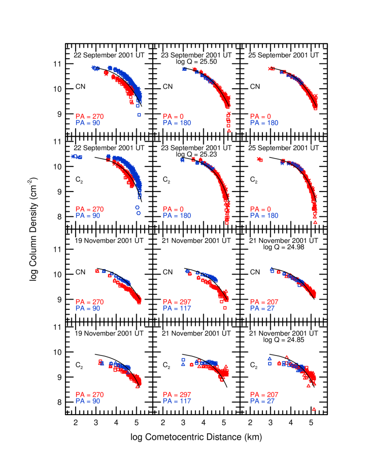
Figure 4: Farnham and Cochran

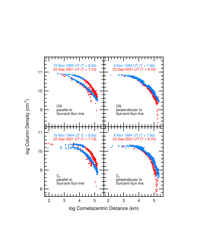
Figure 5: Farnham and Cochran

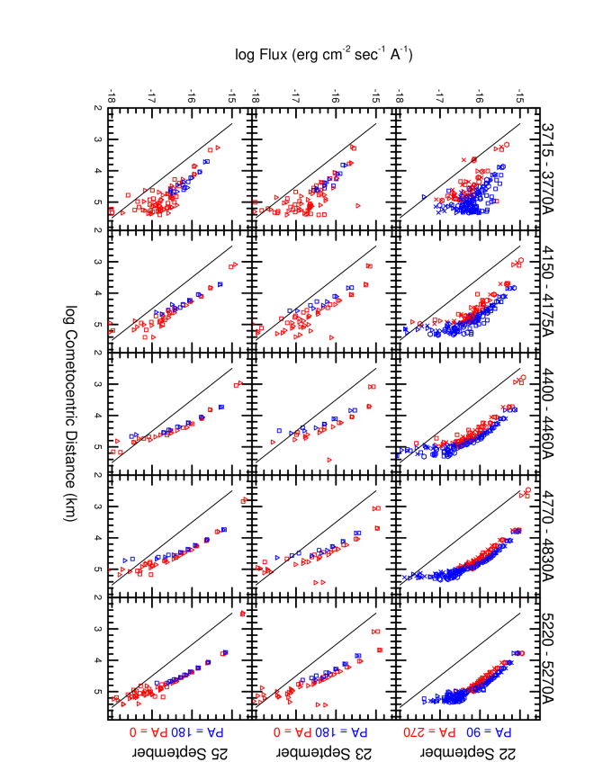
Figure 6: Farnham and Cochran

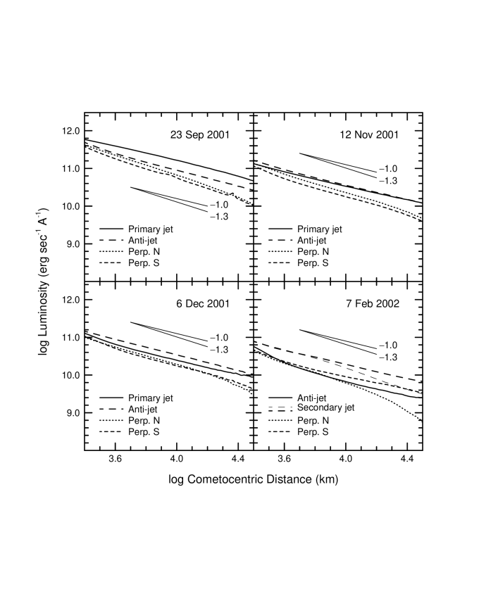
Figure 7: Farnham and Cochran

Figure 8: Farnham and Cochran

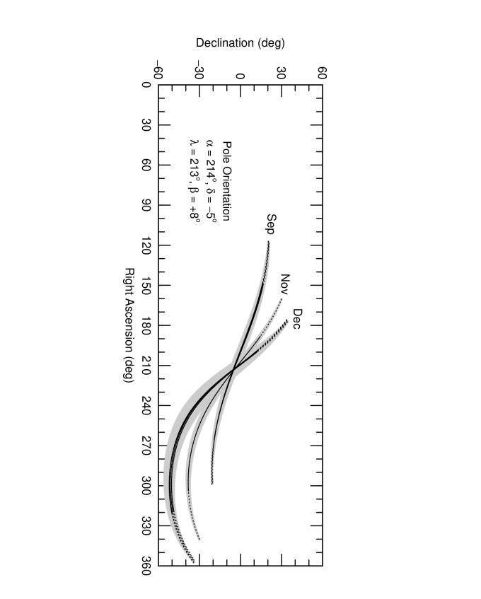
Figure 9: Farnham and Cochran

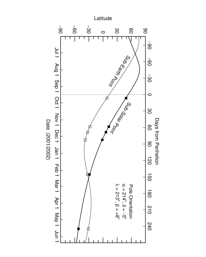
Figure 10: Farnham and Cochran

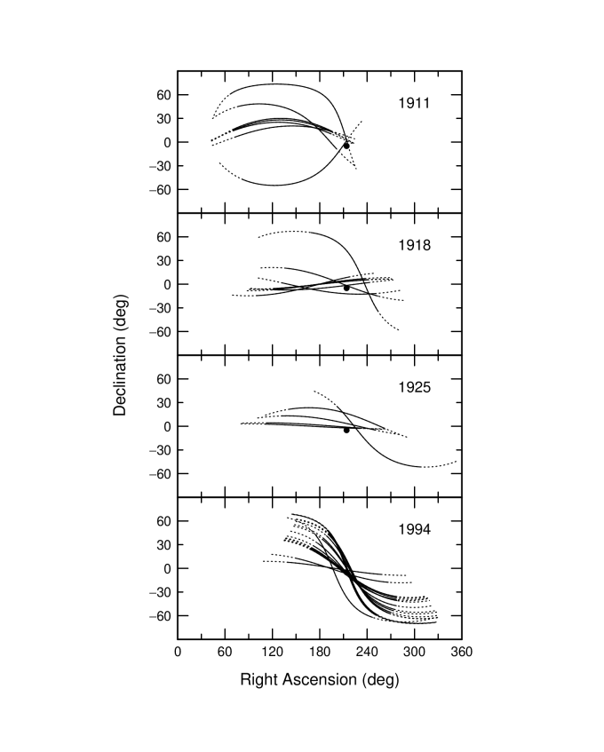
Figure 11: Farnham and Cochran

References

- A’Hearn, M. F., R. L. Millis, D. G. Schleicher, D. J. Osip, and P. V. Birch 1995. The ensemble properties of comets: Results from narrowband photometry of 85 comets, 1976–1992. Icarus 118, 223–270.
- A’Hearn, M. F., D. G. Schleicher, P. D. Feldman, R. L. Millis, and D. T. Thompson 1984. Comet Bowell 1980b. Astron. J. 89, 579–591.
- Cochran, A. L. and E. S. Barker 1999. McDonald Observatory spectroscopic observations of comet 19P/Borrelly. Icarus 141, 307–315.
- Cochran, A. L., E. S. Barker, T. F. Ramseyer, and A. D. Storrs 1992. The McDonald Observatory Faint Comet Survey: Gas production in 17 comets. Icarus 98, 151–162.
- Combi, M. R. 1989. The outflow speed of the coma of Halley’s comet. Icarus 81, 41–50.
- Crifo, J. F. 1991. Hydrodynamic models of the collisional coma. In Comets in the Post-Halley Era (R. L. Newburn Jr., M. Neugebauer, and J. Rahe, Eds.) pp. 937–989 Kluwer Academic Publishers Dordrecht, The Netherlands.
- Donn, B. and J. M. Duva 1994. Formation and properties of fluffy planetesimals. Astrophys. Space Sci. 212, 43–47.
- Donn, B. D. 1990. The formation and structure of fluffy comet nuclei from random accumulation of grains. Astron. Astrophys. 235, 441–446.
- Fulle, M., A. Milani, and L. Pansecchi 1997. Tomography of a sunward structure in the dust tail of comet 19P/Borrelly. Astron. Astrophys. 321, 38–342.
- Haser, L. 1957. Distribution d’intensité dans la têtê d’une comète. Liege Inst. Astrophysics Reprint No. 394.
- Jewitt, D. C. and K. J. Meech 1987. Surface brightness profiles of 10 comets. Astrophys. J. 317, 992–1001.
- Krankowsky, D., P. Lämmerzahl, I. Herrwerth, J. Woweries, P. Eberhardt, U. Dolder, U. Herrmann, W. Schulte, J. J. Berthelier, J. M. Illiano, R. R. Hodges, and J. H. Hoffman 1986. In situ gas and ion measurements at comet Halley. Nature 321, 326–329.
- Lamy, P. L., I. Toth, and H. A. Weaver 1998. Hubble Space Telescope observations of the nucleus and inner coma of comet 19P/1994 Y2 (Borrelly). Astron. Astrophys. 337, 945–954.
- Landolt, A. 1992. UBVRI photometric standard stars in the magnitude range 11.5-16.0 around the celestial equator. Astron. J. 104, 340–371.
- Marsden, B. G. and G. V. Williams 1999. Catalogue of Cometary Orbits. Smithsonian Astrophysical Observatory, Cambridge, MA 13th edition.
- Mueller, B. E. A. and N. H. Samarasinha 2002. Visible Lightcurve Observations of Comet 19P/Borrelly. Earth, Moon and Planets in Press.
- Peale, S. J. 1989. On the density of Halley’s comet. Icarus 82, 36–49.
- Randall, C. E., D. G. Schleicher, R. G. Ballou, and D. J. Osip 1992. Observational constraints on molecular scalelengths and lifetimes in comets. Bull. Amer. Astron. Soc. 24, 1002.
- Rickman, H. 1989. The nucleus of comet Halley – Surface structure, mean density, gas and dust production. Adv. in Space Res. 9, 59.
- Rickman, H., L. Kamel, M. C. Festou, and C. Froeschle 1987. Estimates of masses, volumes and densities of short-period comet nuclei. In Diversity and Similarity of Comets (E. J. Rolfe and B. Battrick, Eds.) pp. 471–481 ESA SP-278.
- Sagdeev, R. Z., P. E. Elyasberg, and V. I. Moroz 1988. Is the nucleus of comet Halley a low density body? Nature 331, 240.
- Samarasinha, N. H. 2002. Cometary Spin States, Their Evolution, and the Implications, Astron. Soc. Pacific Conf. Series: IAU Colloquium 169 in press.
- Samarasinha, N. H. and B. E. A. Mueller 2002. Spin axis direction of comet 19P/Borrelly based on observations from 2000 and 2001. Earth, Moon and Planets in Press.
- Schleicher, D. G., L. Woodney, and R. L. Millis 2002. Comet 19P/Borrelly at Multiple Apparitions: Seasonal Effects in Gas and Dust. Submitted to Icarus.
- Sekanina, Z. 1979. Fan-shaped coma, orientation of rotation axis and surface structure of a cometary nucleus. I. Test of a model on four comets. Icarus 37, 420–442.
- Sekanina, Z. 1993. Effects of discrete-source outgassing on motions of periodic comets and discontinuous orbital anomalies. Astron. J. 105, 702.
- Skorov, Y. V. and H. Rickman 1999. Gas flow and dust acceleration in a cometary Knudsen layer. Planet. Space Sci. 47, 935–949.
- Soderblom, L. A., T. L. Becker, G. Bennett, D. C. Boice, D. T. Britt, R. H. Brown, B. J. Buratti, C. Isbell, B. Giese, T. Hare, M. D. Hicks, E. Howington-Kraus, R. L. Kirk, M. Lee, R. M. Nelson, J. Oberst, T. C. Owen, M. D. Rayman, B. R. Sandel, S. A. Stern, N. Thomas, and R. V. Yelle 2002. Observations of comet 19P/Borrelly by the Miniature Integrated Camera and Spectrometer aboard Deep Space 1. Science 296, 1087–1091.
- Soderblom, L. A., D. C. Boice, D. T. Britt, R. H. Brown, B. J. Buratti, M. D. Hicks, R. M. Nelson, J. Oberst, B. R. Sandel, N. Stern, S. A. Thomas, and R. V. Yelle 2001. Observations of comet 19P/Borrelly from the Miniature Integrated Camera and Spectrometer (MICAS) aboard Deep Space 1 (DS1). Bull. Amer. Astron. Soc. 33, 1087.
- Stone, R. P. S. 1977. Spectral energy distributions of standard stars of intermediate brightness. II. Astrophys. J. 218, 767–769.
- Storrs, A. D., A. L. Cochran, and E. S. Barker 1992. Spectrophotometry of the continuum in 18 comets. Icarus 98, 163–178.
- Wallis, M. K. and A. K. MacPherson 1981. On the outgassing and jet thrust of snowball comets. Astron. Astrophys. 98, 45–49.
- Yeomans, D. K. 1971. Nongravitational forces affecting the motions of periodic comets Giacobini-Zinner and Borrelly. Astron. J. 76, 83–87.