Mixing Time Scales in a Supernova-Driven Interstellar Medium
Abstract
We study the mixing of chemical species in the interstellar medium (ISM). Recent observations suggest that the distribution of species such as deuterium in the ISM may be far from homogeneous. This raises the question of how long it takes for inhomogeneities to be erased in the ISM, and how this depends on the length scale of the inhomogeneities. We added a tracer field to the three-dimensional, supernova-driven ISM model of Avillez (2000) to study mixing and dispersal in kiloparsec-scale simulations of the ISM with different supernova (SN) rates and different inhomogeneity length scales. We find several surprising results. Classical mixing length theory fails to predict the very weak dependence of mixing time on length scale that we find on scales of 25–500 pc. Derived diffusion coefficients increase exponentially with time, rather than remaining constant. The variance of composition declines exponentially, with a time constant of tens of Myr, so that large differences fade faster than small ones. The time constant depends on the inverse square root of the supernova rate. One major reason for these results is that even with numerical diffusion exceeding physical values, gas does not mix quickly between hot and cold regions.
1 Introduction
Measurements of the O/H ratio in the interstellar medium (ISM) along lines of sight reaching altitudes above the galactic disk of up to 1500 pc by Meyer et al. (1998) and Cartledge et al. (2001) suggest that the ISM is well-mixed up to these heights. This suggestion is also supported by the O/H ratios observed in 41 HII regions in M101 (Kennicutt & Garnett, 1996), which show only a 0.1–0.2 dex dispersion about the radial gradient. In NGC 1569 and 4214 the dispersion is extremely low (Kobulnicky & Skillman 1996, 1997). Based on these observations it seems that there exists strong evidence pointing to a fairly well-mixed ISM in galaxies including the Milky Way.
On the other hand, recent observations using the Interstellar Medium Absorption Profile Spectrograph (IMAPS) suggest that there are local variations in the D/H ratio of up to a factor of three among the studied lines of sight (Jenkins et al. 1999; Sonneborn et al. 2000; for an up to date discussion on deuterium abundances see York 2002). The detection of deuterium in the ISM indicates that it was not processed into stars and the local variations reported in the D/H ratio suggest incomplete mixing in the ISM. However, such an inhomogeneous picture contradicts the almost homogeneous distribution seen in O/H ratioes.
Deuterium was produced during big bang nucleosynthesis and is destroyed during the pre-main sequence phase of stars. Thus, its ratio to hydrogen is initially constant in primordial gas and decreases as it is processed in stars. Deuterium may also be added into galactic interstellar gas by accretion of primordial gas, as required by some chemical evolution models in order to explain its present abundance in the Galaxy (see Tosi et al. 1998 for details.). Mulan & Linsky (1999) proposed that deuterium could be formed in stellar flares from M dwarf stars. However, the production of deuterium by this mechanism should be accompanied by a significant production of lithium, which has not been observed.
Contrary to oxygen, deuterium has a primordial origin and limited destruction mechanisms, making this species a good tracer of the mixing in the ISM. Abundances of deuterium are probably not influenced by depletions onto grains, as is the case with most other species. Although there has been some suggestion that deuterium may be preferentially bonded onto the surfaces of dust grains, this effect is not sufficient to explain the large variations in D/H seen in the ISM. Furthermore, deuterium and oxygen are the only species that have an ionization fraction that closely follows that of H. Deuterium and hydrogen have almost the same ionization potentials, photoionization cross sections and recombination coefficients, making it difficult for the D/H variations to be a result of any unusual ionization effects. Other effects such as fractionation by molecular chemistry have been considered by different authors, but there is no strong evidence that such effects can be responsible for the D/H variations seen in the ISM.
We face a set of observations that point towards contradicting conclusions. O/H observations support the idea that complete mixing occurs in the ISM on timescales comparable to those for chemistry to reach equilibrium, while D/H measurements indicate a not so well mixed ISM. Solving this contradiction is an important step towards the understanding of the mixing and variation of these elements in the ISM, and therefore, of the the interpretation of local measurements as constraints of its cosmic abundance.
Roy & Kunth (1995) discussed the problem of mixing in the ISM and concluded that the ISM should appear more homogeneous than it does. These authors suggested that mixing in the ISM is driven by three main mechanisms acting on different length scales. On the Galactic scale, they argued that turbulent diffusion of interstellar clouds in the shear flow of galactic differential rotation could remove the inhomogeneities in the ISM in less than yr, in particular the fluctuations seen in O/H. At scales of pc, cloud collisions and expanding supershells driven by supernovas (SNs) from evolving massive star associations, differential rotation and triggered star formation (by stellar winds and SN explosions) could re-distribute and mix inhomogeneities efficiently in about yr; and at smaller scales of the order of pc, turbulent diffusion may be the dominant mechanism in cold clouds, while Rayleigh-Taylor and Kelvin-Helmoltz instabilities could develop in regions of gas ionized by massive stars, leading to complete mixing in less than 2 Myr. (This analysis does not take into account that during the mixing process new inhomogeneities are added into the ISM.)
Bateman & Larson (1993) already pointed out that turbulent mixing should be important in the ISM. However, they based their analysis on a picture of cloud collisions that ignores the likely origin of clouds as density enhancements in regions of converging flow in the turbulent ISM (e.g. Vázquez-Semadeni et al. 1995).
Tenorio-Tagle (1996) noted that classical diffusion theory on the molecular level predicts mixing timescales in the ISM for gas with K several orders of magnitude longer than that proposed by Roy & Kunth (1995). As a consequence, Tenorio-Tagle (1996) concluded that turbulent mixing as well as hydrodynamical instabilities, as proposed by Roy & Kunth (1995), are important mixing mechanisms that allow the reduction of the long mixing time scales obtained from classical diffusion theory.
The observations showing that the ISM has an inhomogeneous distribution pose the question of how it is possible in a SN-driven ISM for different species not to be mixed well enough to suppress local variations of their ratio to hydrogen along and among lines of sight. The ISM is regulated by SN explosions, and therefore, by well-structured and explosive flows rather than just by diffuse turbulence that acts on the smaller scales. To understand the mixing process in such a medium we carry out direct numerical simulations of the evolution of the ISM polluted with inhomogeneities of different length scales. We aim to understand if classical mixing length theory can be used to predict the mixing time scales as a function of size scale.
In § 2 we review the existing theoretical ideas on dispersion, diffusion and turbulent mixing and apply them to the ISM. Section 3 describes the modified version of the three-dimensional model of de Avillez (2000), how the runs used in the current study were set up, and the global evolution of the ISM as seen in these simulations. In § 4, the evolution of the tracer fields and the mixing process in the ISM are described. Section 5 discusses the results and their implications. Finally, § 6 presents a summary of the main results and final remarks.
2 Dispersion, Diffusion and Turbulent Mixing in the ISM
The ISM is a turbulent medium with inhomogeneous makeup driven by SN explosions. The dominance of SN explosions was deduced by Cox & Smith (1974) and McKee & Ostriker (1977) from the detection of hot gas in UV absorption lines and X-ray emission. That these explosions interact to drive a turbulent flow was demonstrated numerically by Rosen & Bregman (1995). The nature of that flow in three dimensions has been explored with high-resolution hydrodynamical simulations by de Avillez (2000) and de Avillez & Berry (2001), while Korpi et al. (1999a, 1999b) included the effect of magnetic fields, at lower resolution. The SN explosions individually and collectively transport hot gas over large distances in more or less laminar flows. Turbulence driven by the interactions of these flows forms eddies that mix the gas on smaller scales. On the smallest scales molecular diffusion finally completes the mixing process.
2.1 Molecular Diffusion
Molecular diffusion is the consequence of frequent, stochastically distributed collisions between gas particles. The individual particles scatter in a random walk around their initial location. The total squared displacement of a particle
| (1) |
where is the diffusion coefficient given by
| (2) |
is the root mean square velocity of the particles, and is the mean free path of the particles. The distribution of the particles over time can be described by a Gaussian distribution with a standard deviation around the initial location of the particles.
If collisions happen in a homogeneous gas enclosed in a fixed volume, the relevant quantity to describe the diffusive process is the mean free path. It does not make sense to talk about a diffusion coefficient or an expected displacement because, viewed from the outside, the collisions do not change the properties of the gas, only the positions of the individual molecules.
The situation is different if there is a composition gradient. Then there are more particles of the species under study in one part of the volume than in the other. A random walk carries more particles out from the higher density region than in from the lower density region. Net transport results, reducing the gradient and eventually leading to a homogenized distribution. The streaming of particles can be described as
| (3) |
with being the diffusion tensor for anisotropic diffusion and the number of particles per unit volume. The gradient is the driving force for the flow, so a larger gradient leads to a larger flow. The flow also depends on the mobility of the particles, described by the diffusion tensor. Since the diffusion tensor depends on the particle speed and on the mean free path, for a given gradient, the streaming , as well as the average displacement , are largest for fast particles undergoing few collisions (thus having a large mean free path) and smallest for slow particles undergoing many collisions.
If the diffusion is isotropic, the diffusion tensor reduces to a diffusion coefficient and the streaming becomes . From the conservation of mass one derives the diffusion equation
| (4) |
If the diffusion coefficient is also independent of the spatial coordinate the equation can be reduced to
| (5) |
This equation shows that the characteristic diffusion time over a typical length , is
| (6) |
The time evolution of the particle density being transported, say along the direction, is given by
| (7) |
where is the initial particle distribution.
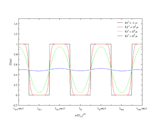
Let us now consider diffusion of an idealized checkerboard pattern with square size subject to diffusion with an isotropic, uniform diffusion coefficient . In one dimension, the pattern can be described as a square wave in composition along the -axis with wavelength (see Figure 1), so that at ,
| (8) |
where , and , The square wave evolves following the solution given in equation (7)
| (9) |
where the solution must satisfy the periodic boundary condition , and the integral has the final form
| (10) |
where , is the error function,
| (11) |
and if we use a scale of parsecs for and years for , the value of the constant , with cm2 s-1. Figure 1 shows the time evolution of the solution (9) for a medium having inhomogeneities with a scale length of , where is a scale length of reference. The solution is given in units of , with again taken to be in parsecs.
The mixing time scales vary as , where is the time of evolution of a reference square wave with length pc. This result is a direct conclusion from the diffusion timescale. As an example, in a medium with cm2 s-1 subject to mixing according to a diffusive mixing length theory, inhomogeneities with length scale of 100 pc would be erased in a time of yr, while those with a length scale of 1 kpc would be erased in a time of yr.
2.2 Turbulent Mixing
Turbulent diffusion occurs when gas is stirred by more or less random forces, forming eddies within which local composition gradients increase, enhancing local molecular diffusion.
Studies of isotropic, homogeneous, incompressible turbulence led to the classical Kolmogorov (1941) cascade picture of turbulent flows. Eddies with a certain size are assumed to have some typical velocity associated with them. The corresponding Reynolds number will be larger for larger eddies, so viscosity is not very important for them. The energy cascades from these large eddies to smaller ones. The size of the smallest eddies is set by the condition . Thus, the minimum size of an eddy is
| (12) |
and the energy in these eddies is lost to viscous dissipation. Energy is fed at some rate per unit mass per unit time to the largest eddies of size and velocity with respect to neighboring eddies, for which the Reynolds number . This energy then cascades to smaller and smaller eddies until it reaches eddies with the smallest size possible, , which dissipate the energy at the same rate as they are fed in order to maintain equilibrium. Energy does not accumulate at any scale; the intermediate eddies merely transmit this energy to the smaller eddies in a cascade. These intermediate eddies are characterized by their size and velocity . Energy passes through the cascade at a constant rate , independent of wavenumber (Kolmogorov 1941). The velocity of the eddies scales as
| (13) |
resulting in an eddy lifetime
| (14) |
where is the wavenumber. Thus, the time taken by an eddy to disappear varies as . An eddy of scale length , in units of 100 pc, exists for a time
| (15) |
where is written in units km s-1. We can estimate the time scale for mixing of hot gas using this classical eddy turnover time. Taking as the root mean square velocity of the hot ( km s-1) gas and assuming that the eddies have a length scale pc, the time scale for complete mixing to occur is roughly 1 Myr. Therefore, if incompressible turbulent mixing dominates the mixing process, hot regions will mix very quickly.
2.3 Dispersal
Dispersal describes the transport of gas across large regions by laminar flows, such as those within SN remnants or superbubbles. On a large enough scale, encompassing many regions of laminar flow, dispersion can still be treated as a diffusive process that satisfies the diffusion equation (5) with replaced by the average density of the ensemble of transported particles . In this case it does not make sense to speak about the different phases of the transported gas, because all of it is dispersed with the flow, and therefore, the mean free path , of the molecular diffusion, is replaced by a mixing length path , which is defined as the distance over which the ensemble of particles is transported before it halts. Note that it no longer makes sense to define the rms velocity of each gas component in the transported flow separately, because the whole ensemble is transported roughly at the same speed.
According to this approximation, the diffusion timescale of a system with parsec-scale motion can be written as
| (16) |
where is the length over which the ensemble of particles is transported, in units of parsecs; is the diffusion coefficient, written in units of cm2 s-1; and is the root mean square velocity of the emsemble of particles being transported. If one assumes that the characteristic length scale over which the flow is transported is the same as its mixing length, then the diffusion time scales as
3 Simulations
3.1 Supernova-Driven ISM Model
To study the mixing timescales in the ISM we added tracer fields to a modified version of the three-dimensional, SN-driven, ISM model of Avillez (2000). The model is run with an adaptive mesh refinement (AMR) hydrodynamics code on a kpc region of the Galactic disk. It includes a fixed gravitational field provided by the stars in the disk, radiative cooling assuming optically thin gas in collisional ionization equilibrium, and uniform heating due to starlight. The radiative cooling function is a tabulated version of that shown in Figure 2 of Dalgarno & McCray (1972) with an ionization fraction of 0.1 at temperatures below K and a temperature cutoff at 10 K. Background heating due to starlight varies with as described in Wolfire et al. (1995) and is kept constant in the directions parallel to the plane; in the Galactic plane at it is chosen to initially balance radiative cooling at 8000 K. The presence of background heating leads to the creation of thermally stable phases in the ISM. Due to the presence of a stable phase at low temperatures, the amount of cold gas seen in these simulations is larger than that found in the simulations presented in Avillez (2000).
The interstellar gas is initially distributed in a smooth disk with the vertical distribution of the cool and warm neutral gas given by Lockman et al. (1986) and summarized in the Dickey & Lockman (1990) distribution. In addition, an exponential component representing the distribution of the warm ionized gas with a scale-height of 1 kpc in the Galaxy is included, as described in Reynolds (1987). The model includes supernovae types Ib+c and II. Supernovae of type Ia are not included in these simulations because their role is not important in the mixing process that occurs near the Galactic plane, although they may be important in the disk-halo interaction due to their scale-height.
The rates of occurrence of SNe types Ib and Ic in the Galaxy are yr-1, while those of type II occur at yr-1 (Cappellaro et al. 1997). We take the total rate of these SNe in the Galaxy to be yr-1, corresponding to a rate of one SN every 71 yr. These rates are normalized to the volume of the stellar disk in which a specific SN type is found: a galactic radius of 12 kpc is assumed for all stellar disks, but their half thicknesses are assumed to be twice the scale height of the corresponding SNe distributed in the field. In particular as SNe Ib+c and II are assumed to have the same scale height then their stellar disks have the volume pc3.
SNe of types Ib+c, and II are explicitly set up at the normalized SN rate, with 40% of them placed at random locations distributed in an exponential distribution with a scale height of 90 pc, and 60% in locations where previous SNe occurred, representing OB associations, in a layer with a scale height of 46 pc following the distribution of the molecular gas in the Galaxy.
The first SNe in associations are chosen to occur in locations where the current local density is greater than 1 cm-3. No density threshold is used to determine the location where isolated SNe should occur, because their progenitors drift away from the parental association and therefore, their site of explosion is not correlated with the local density. Similarly, later SNe in associations are no longer determined by gas density.
The SNe are set up at the beginning of their Sedov phases, with radii determined by their progenitor masses, which are injected into the location of the explosion. Type II SNe come from early B stars with masses while type Ib+c SNe have progenitors with masses (Tammann et al. 1994). In this model the maximum mass allowed for an O star is 30 . Avillez (2000) describes in detail the algorithm used to set up the isolated and clustered SNe during the simulations.
3.2 Numerical Method and Boundary Conditions
These simulations use the piecewise-parabolic method of Colella & Woodward (1984), a third-order scheme based on a Godunov method implemented in a dimensionally-split manner (Strange 1968) that relies on solutions of the Riemann problem in each zone rather than on artificial viscosity to follow shocks. The Godunov approach is typical of standard numerical techniques in regions where the solution is smooth. However, in regions with discontinuities, such as strong shocks, the Godunov method approximates the solution well by analytically solving an associated Riemann problem. This is an idealized problem describing the evolution of a simple pressure jump into shocks and rarefactions, with a contact discontinuity in between. Monotonicity constraints ensure that these discontinuities remain sharp and accurate as they traverse the computational grid. The higher-order spatial interpolation in the PPM allows steeper representation of discontinuities.
During the simulation, the mesh is refined periodically in regions with sharp pressure variations using the AMR scheme. The local increase of the number of cells corresponds to an increase in linear resolution by a factor of two (that is, every refined cell is divided into eight new cells). At every new grid the procedure outlined above is carried out, followed by the correction of fluxes between the refined and coarse grid cells. The adaptive mesh refinement scheme is based on Berger & Colella (1989), but the grid generation procedure follows that described in Bell et al. (1994).
The computational domain has an area of 1 kpc2 and a vertical extension of 10 kpc on either side of the midplane. In the simulations discussed here, AMR is used in the layer pc. In the highest resolution runs, three levels of refinement are used, yielding a finest resolution of 1.25 pc. For pc the resolution is 10 pc. Periodic boundary conditions are used on the side boundaries, while outflow boundary conditions are used on the top and bottom boundaries.
3.3 Tracer Field Implementation and Mixing Runs
To follow how composition differences mix, we use a tracer field. A tracer field acts as a drop of ink in a fluid. In time the drop will spread and eventually mix completely into the fluid. This occurs because thermal motion leads to collisions between ink and fluid molecules, distributing both species uniformly. The simulations do not include any physical diffusion term, however, so contrary to what happens in a real fluid or gas, the mixing of the tracer field occurs by numerical diffusion, which will generally be faster and larger scale than the physical diffusion in astrophysical problems. As a consequence the mixing time of a tracer field in our model provides a rather strong lower limit for the timescale of mixing resulting from physical diffusion.
The tracer field is an intensive scalar whose advection is computed with the same algorithm as the density. We initially set its value to be either one or zero to represent regions of different composition. In the absence of diffusion, either numerical or physical, these values would remain fixed as the gas is advected. In the presence of diffusion, the tracer field values will change. In our simulations, this is a result of the numerical diffusion present in the Godunov advection scheme.
This scheme assumes that the flow solution is represented by a series of piecewise constant states, and therefore, that the numerical representation approximates the true solution near discontinuities. The numerical solution is evolved by considering the nonlinear interaction between these piecewise constant states. Viewed in isolation, each pair of neighbouring states constitutes a Riemann problem. The algebraic solution in the overall grid results from a collection of Riemann problems for all the interfaces between two sucessive cells at every time step. The discontinuity between two states evolves into some combination of shock and rarefaction waves, separated by a contact discontinuity (Figure 3). The tracer field is advected in the same way as the density and therefore, it diffuses between any rarefaction wave and the contact discontinuity formed as a result of the Riemann problem solution. This process happens between every pair of neighboring cells, leading sooner or later to a change of the tracer field value. In the case at hand we use tracer fields to follow the evolution and mixing of composition differences in the ISM. As mixing occurs by numerical diffusion, regions with values intermediate between zero and unity grow, until ultimately the entire volume is filled with gas having value roughly 0.5.
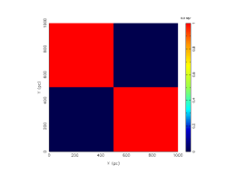
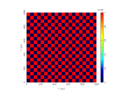
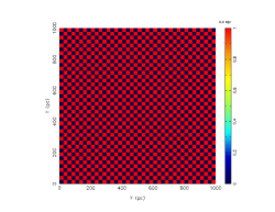
The tracer field is set up initially with values of and 1 on alternating squares of a checkerboard in the plane of the Galaxy with square sides of or 500 pc (Figure 2). The 500 pc scale corresponds to a tracer field that fills a quarter of a 1 kpc length square board. The distribution is uniform in the vertical direction; that is, the squares are extended into rectangular solids of uniform composition vertically. This setup allows a direct comparison to the analytic solution given in § 2.1 for the mixing of inhomogeneities of different length scales in the ISM due to classical turbulent diffusion.
In the current work we report on simulations using seven SN rates , 5, 10, 15, 20, 30 and 50, having finest grid resolutions of 1.25, 2.5 or 5 pc. In general, the simulations were stopped between 50 and 70 Myr after complete mixing occurred. The simulations ran for 400 Myr for , 300 Myr for , and 200 Myr for the remaining SN rates. A summary of these runs is presented in Table 1.
4 Results
4.1 Overview of Results
In the first 50 Myr the system evolves into a statistical steady state on the global scale. Once disrupted by SN explosions, the disk never returns to its initial state, provided SNe continue to explode. Instead, regardless of the initial vertical distribution of the disk gas, a thin disk of cold gas forms in the Galactic plane, and, above and below, a thick inhomogeneous gas disk forms. Gas flows between the thin and thick gas disks, with upward and downward flowing gas coming into dynamical equilibrium. The upper parts of the thick disk form the disk-halo interface, where a large scale fountain into the halo is driven by hot ionized gas escaping in a turbulent convective flow from the disk-halo interface and from superbubbles blowing out of outer layers of the thin disk.
Table 1 gives the time for complete mixing, measured in the supernova forming stellar disk, which we take to be the time needed for the average value of the tracer field to saturate at a value (see §4.2). Results are shown for checkerboards with initial square sizes of , 50, and 500 pc, and SN rates /, 5, 10, 15, 20, 30, and 50, at resolutions of the finest grid levels used during adaptive mesh refinement. A quick look at the table shows that the time required for complete mixing of inhomogeneities with and pc differs by only 5–20 Myr, while that for inhomogeneities with pc is larger by, at most, another 20 Myr. These differences decrease with increasing SN rate. Runs with different finest resolution for the same SN rate show similar mixing time scales, suggesting that the results depend quite weakly on the actual strength of the diffusion.
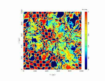
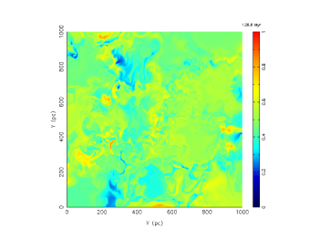
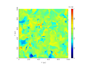
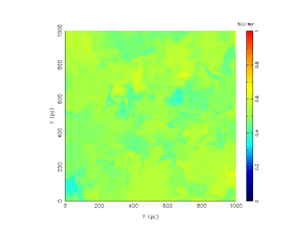
Figures 4 and 5 present snapshots of the evolution of tracer fields in checkerboards with initial length scale of pc and SN rates , 5 and 15. The snapshots in Figure 4 were taken at 50 and 126.6 Myr, while those in Figure 5 were taken at 50 Myr of evolution. The resolution of these snapshots is 1.25 pc in Figure 4 and 2.5 pc in Figure 5. We see that for the Galactic SN rate, the mixing process at 50 Myr is just starting to occur, while for larger SN rates, it is well advanced, with a larger fraction of the inhomogeneities reduced to weak structures that take a long time to be erased. For example, in the model with at a time of 50 Myr, the tracer field has a value varying between 0.4 and 0.6. For the other rates shown in the figures at 50 Myr there are still unmixed regions where tracer field has values of zero or one.
These Figures show large-scale laminar flow in the hot gas bubbles that transports tracer field over large distances. The expansion and interactions of the bubble drive shocks into the warm and cold gas. Vorticity generated at shock intersections drives eddies mixing the gas up to 100 pc scales, as well as Rayleigh-Taylor fingers that degenerate into smaller eddies at the tips of their caps. The eddies cascade from intermediate to small scales, further mixing the tracer field down to the diffusion scale. The mixing process thus proceeds by different mechanisms at different scales, because of the inhomogeneous, compressible nature of the flow.
The mixing process is independent of the spatial distribution of isolated SNe that occur randomly in the field. The locations of type II and Ib+c SNe occurring away from their parental OB associations are determined from a file of random numbers chosen at the beginning of a simulation. We ran simulations with different sets of random numbers and finest grid resolutions of and 2.5 pc, and found mixing time scales virtually the same as the ones reported here, so we do not further discuss those models.
4.2 Average, Variance, and Maximum
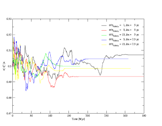
The simulations start with exactly the same number of cells having value 1 and 0. Therefore, the average value of the tracer field, at . By definition complete mixing occurrs when the tracer field at any point in the grid has . However, due to round-off and phase errors of the numerical scheme, the actual value for completely mixed material may differ from 0.5 by a few percent. Once the tracer field has this constant value on the entire grid, no further variation occurs.
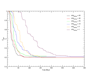
Figure 6 shows the time variation of for three SN rates and 15, and for two finest grid resolutions of 2.5 and 5 pc. During the first 50 Myr, shows small variations around 0.5, approaching a constant value as mixing increases and the small scale structure dominates the mixing process. The initial variations of result from the increased error occurring as steep color gradients interact with steep velocity gradients in SN-driven shock waves. As the color is mixed, the color gradients decrease, and approaches a constant value close to 0.5. The biggest errors, still only 2.4%, occur for the highest SN rates, where strong shocks are more widely distributed.
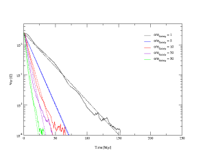
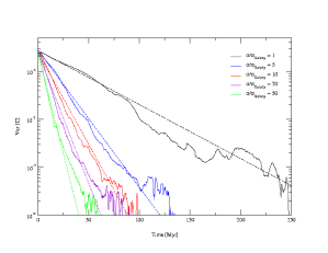
The average value of gives an indication of the time at which complete mixing occurred, but it does not provide any information of the mixing process. Further information may be obtained from the variance of the tracer field, . This evolves from at to when complete mixing occurs. The variance has a steady decrease with time until it reaches a value of . For the decrease is no longer steady, but rather sporadic, suggesting that we have reached a regime where numerical noise is dominating. Figure 7 shows the variance of (for ) over time for inhomogeneities with different length scales, along with exponential fits to the steady decrease of until it reaches a value of . The fits shown are for the shorter length scales of the inhomogeneities. We find that the variance of the tracer field for inhomogeneities with length scales and 50 pc decays to remarkably close to exponentially, with . For such decrease is seen for or 5 if pc and if pc.
Figure 8 shows the variation of the time constant with SN rate for inhomogeneities with initial and 50 pc, as well as the best power-law fits to the data points. The fits to an inverse square root law are remarkably good, with correlation coefficients of 0.997 and 0.998 for and 50 pc, respectively. For length scale of 50 pc,
| (17) |
In future work we will extend our parameter study sufficiently to define the dependence on inhomogeneity length scale fully.
This exponential decay law indicates that large variations in the tracer field decay quickly while smaller variations last much longer. Such a decay law for the variance of breaks down for larger inhomogeneities, and in particular it does not apply for inhomogeneities with pc. The extended parameter study should show at which length scale the deviation from this behavior begins to occur. We will also examine whether this result extends to smaller scales using finer grids.
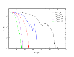
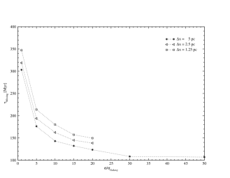
The time variation of the maximum value of the tracer field, is shown in Figure 9. The exponential decay behavior is again seen, with a fast initial decline followed by a slow approach to complete mixing. Structures with small variations in composition will thus be present for extended periods of time. The figure also shows that the time taken for complete mixing to occur decreases with increasing SN rate until it saturates for . This result is also seen in the variation of the mixing time with SN rate shown in Figure 10, which shows that for SN rates the mixing time scales differ by only a few Myr.
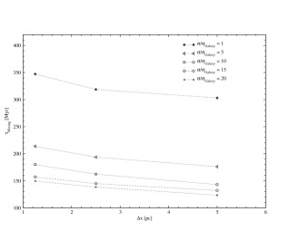
The mixing process has a rather weak dependence on the resolution used in the calculations, and thus of the actual strength and scale of diffusion. Running the scheme with a better resolution decreases the numerical errors, and therefore also the magnitude of numerical diffusion. Therefore, the mixing times become longer (going from right to left column in Table 2), but this increase is far slower than the increase in resolution, and declines with increasing resolution, as shown in Table 2 and Figures 11 and 10. This demonstrates that numerical convergence is occurring, and further that unresolved details of the mixing process at small scales do not affect the behavior at resolved scales. This appears to be because the mixing process depends primarily on motions near the SN driving scale of pc, with the presence of small scale diffusion more important than its exact properties.
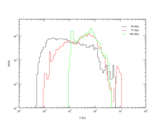
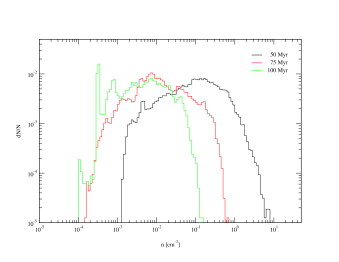
The similarity in the mixing time scales for occurs because for SN rates higher than this the entire disk quickly heats. Figure 12 shows the temperature probability distribution functions (PDFs) of the disk gas for . After the first 50 Myr of evolution a large fraction of the disk gas already has temperature K and by 100 Myr of evolution all the gas has reached at least K. As a consequence of the high SN rate the disk becomes warmer and cooling becomes inefficient. The high rms velocities in this hot gas lead to quick mixing, as in hot regions in less energetic models. The complete lack of colder regions, however, means that all the gas mixes on the same short time scale. Once there is no further cold gas, increasing the SN rate further only slowly increases the rms velocity, leading to the saturation behavior seen.
We emphasize that classical mixing length theory badly fails to predict the mixing time scales that we compute. That theory predicts that the mixing time scales should depend on the length scales. That is, let a checkerboard be composed of squares with length scale , and the squares be further divided into smaller squares with length scale . Then mixing length theory would predict the diffusion time scales of these squares to be related by for constant diffusion coefficient. Thus, the predicted ratios of timescales (for example for and in parsecs) are and . However, Table 1 shows that the actual ratioes are never greater than 1.2, a value far smaller than predicted.
4.3 Profiles
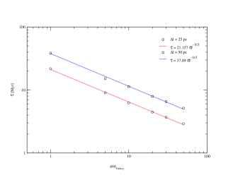
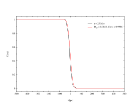
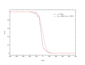
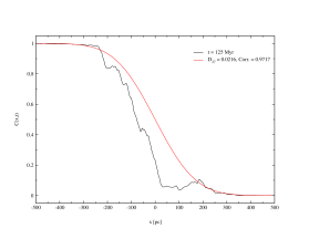
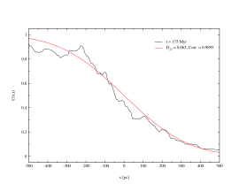
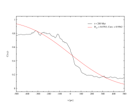
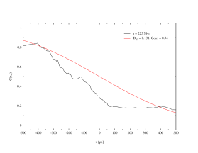
Another approach to measuring the mixing timescale is to directly compute the diffusion coefficient required to fit the average profile across an initially sharp color gradient, using the analytic theory of § 2.1. Figure 13 presents profiles of the tracer field averaged along the -axis for pc for the checkerboard with squares of initial length of 500 pc (shown in the top panel of Figure 2), overlaid by the classical diffusion solution from equation (10) with . Initially the solutions fit the average profile of the tracer field well, but at later times the fits become somewhat worse. The correlation factors of these fits reduces as time evolves from 0.998 at 25 Myr to 0.94 at 225 Myr.
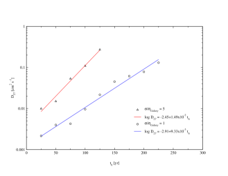
From the fits, we can deduce the diffusion coefficient written in units of cm2 s-1. The time variation of D27 for two different SN rates is shown in Figure 14. The straight lines are the best fit to the data points. We find that the diffusion coefficient varies exponentially with time, with the general expression of
| (18) |
where, if is given in Myr, and Myr for , and and Myr for . If the mixing were regulated by classical diffusion, then we would expect that the diffusion coefficient would be nearly constant or vary around a mean value with time, rather than exponentially increasing.
5 Discussion
In this paper we try to understand how long it takes to erase inhomogeneities in the ISM and if this process depends on the inhomogeneity length scale. That is, does it take longer to mix big regions than small ones? We modified the three-dimensional model of Avillez (2000) to incorporate tracer fields and ran simulations with different SN rates, distributions of SNe in the field, and numerical resolutions. (Clustered SNe from OB associations are explicitly set up, with the first SN in an association occurring in a location where the local density is greater than 1 cm-3.)
The three-dimensional adaptive mesh refinement code used in our simulations, unlike 1-zone chemical evolution models (Matteucci et al. 1999; Tosi et al. 1998) and chemodynamical models (Samland et al. 1997; Samland 1998; Argast et al. 2000, to name a few), enables us to resolve local inhomogeneities in the ISM with a spatial resolution as good as 1.25 pc. This allows us to test the usual assumption of Galactic chemical evolution models that assume instantaneous mixing of the ISM at all times. Mixing in the real world takes finite time, and ultimately occurs on the molecular scale, through physical diffusion. We set a lower limit on the mixing time scale by assuming that it is set at the far larger grid scale by faster numerical diffusion. We find that the actual value of the mixing scale does not strongly influence the mixing timescale.
Matter can enter and leave the section of the Galaxy under study through the top and bottom outflow boundary conditions, as well as moving to neighboring periodic boxes (eg passing through a periodic side boundary condition), although we do not yet include Galactic rotation in our model. Chemical evolution models do not normally allow radial transport of matter between different rings, but it occurs in our models.
Because the domain extends to 10 kpc on both sides of the midplane, gas can cycle between the disk and the halo in a Galactic fountain as a result of the dynamics of the flow in the gravitational field of the Galaxy (see Kahn 1981; Avillez 1999). The mixing time scales of the disk gas are regulated mainly by the SNe, because the disk gas that enters the disk-halo cycle takes some 200 Myr to return to the disk (Kahn 1981). Furthermore before reaching the thin gas disk, the descending gas hits the thick gas disk and decelerates due to drag (Kahn 1981; Benjamin & Danly 1997). Therefore, most of the descending gas will not contribute strongly to the mixing process of the ISM with pc.
This work only studies the mixing process as a way of erasing inhomogeneities in the ISM. It does not take into account continuing pollution of the ISM by SNe, planetary nebulae, and stellar winds, which we will study in future work. The actual enrichment of the disk gas depends on the sources and the efficiency of mixing. If the ejected metals are quickly distributed over a large volume, spatially homogeneous enrichment takes place. If the mixing volume is small, the ISM in the vicinity of a SN will be highly enriched, while large parts of the disk remain metal-poor until the gas mixes out on time scales of hundreds of Myr or more. In this case the ISM may remain chemically inhomogeneous, with newly formed stars having different compositions depending on where they form. Over gigayear timescales, mixing does appear to be quite effective over scales of many kiloparsecs.
This work shows that inhomogeneities that are present in the ISM, assuming that no further inhomogeneities are introduced into the system, can take a long time to be erased. If inhomogeneities are introduced at a time larger than the time scale for mixing, the system will show temporarily an homogeneous state, which ends when inhomogeneities are introduced. On the other hand, if inhomogeneities are introduced on a time scale smaller than the mixing time, then the system will show an inhomogeneous distribution during its evolution. Therefore, from the simulations we conclude that for the ISM to show a homogeneous distribution, no inhomogeneities should be introduced over periods of roughly a hundred megayears. This is longer than typical star formation time scales, so new SNe and pre-main sequence stars can continue to maintain an inhomogeneous composition so long as star formation continues.
The rate at which inhomogeneities are erased increases with the SN rate to values about ten times greater than the Galactic rate. Above that rate, no cold medium remains, mixing occurs quite quickly, but above this threshold, further increasing the SN rate does not markedly further increase the mixing efficiency.
The time for complete mixing is already longer than any time scale for chemical equilibrium to occur and therefore the ISM will show an uneven distribution. Even if the major fraction of the ISM gas is completely mixed, lower level inhomogeneities will still be seen as abundances are measured more carefully. Furthermore, as the mixing time scales are longer than the time interval for SNe type II to occur and enrich the ISM with metals, low-level inhomogeneities are continuously maintained, leading to a poorly mixed ISM, except in the hot regions where the mixing process is fast (of order 50 Myr).
For a galactic SN rate, the ISM is likely fairly inhomogeneous, since the SNe are spatially well separated and erasing these inhomogeneities takes a long time (of the order of 350 Myr). A single SN event can thus substantially influence its surroundings. If we consider, for example, a 20 pc sphere with number density around a SN with 1 M⊙ of metals in its ejecta, the ejecta represent a fraction of the metals in the region. Thus, individual SNe can drastically change the local metallicity in low metallicity gas. Stars formed before mixing has finished can have a wide range of metallicities; further work will be needed to make quantitative predictions of the expected dispersion for comparison with observations, however.
The smallest mixing time scale that we find in our study is Myr and occurs for . After some of the gas has been mixed, the simulations show that the ISM remains inhomogeneous for at least twice as long on scales smaller than a kpc. Even when the rate of SNe is increased to ten times the Galactic rate, this uneven abundance distribution structure takes tens of Myr to disappear.
At the finest grid scale we suppress the turbulent diffusivity, as numerical viscosity becomes the dominant diffusion mechanism. At these scales there would physically be a continuing turbulent mixing that we do not resolve. The resolution study shown in Figures 10 and 11 demonstrates, however, that the mixing time is practically independent of the actual value of the diffusion scale. Changing the linear diffusion scale by factors of as much as four produced less than 20% changes in the diffusion time. This means that we can effectively assume that the mixing is dominated by an inertial scale decoupled from the diffusion scale, so that the details of how the diffusion occurs do not affect the larger-scale behavior.
6 Summary and Final Remarks
The main results of this study are:
-
•
The mixing of a SN-driven ISM is characterized by three regimes: laminar flows dominate on scales close to a kpc, turbulent mixing dominates below about a hundred parsecs, and diffusive processes finally dominate at the smallest scale.
-
•
Mixing at the larger scales appears nearly independent of the exact value of the diffusive scale, so long as some diffusive process ultimately operates at small scales.
-
•
The time scale to erase inhomogeneities in the ISM on length scales from parsecs to kiloparsecs is nearly independent of the length scale; classical mixing length theories badly fail to describe this behavior.
-
•
The time scale for complete mixing, providing no further inhomogeneities are introduced, is some 350 Myr for the Galactic SN rate, decreasing with increasing SN rate up to a threshold value. Above this threshold value, further increases in the SN rate have little further effect.
-
•
The speed of mixing decreases almost exponentially, with a time constant dependent on the inverse square root of the SN rate: strong inhomogeities decay quickly, while weaker ones last much longer.
-
•
The diffusion coefficient derived from fits of a solution of the diffusion equation to the simulation results does not remain constant as assumed by classical mixing length theory, but rather increases exponentially with time, with a time constant dependent on the SN rate.
This work is far from complete. At least four issues clearly remain to be addressed. First, we need to determine the actual length scale at which the exponential decrease in tracer field variance ceases, somewhere between 50 and 500 pc. Second, if further inhomogeneities are introduced, such as the chemical elements fed into the ISM by SNe, planetary nebulae, and stellar winds, large parts of the ISM, or indeed the whole ISM, may never reach homogeneity. Even though stronger inhomogeneities decay quickly, the exponential decline in mixing rate for weaker inhomogeneities means that a wealth of weaker inhomogeneities will remain. Determining quantitative values of the dispersion of metallicities will help solve outstanding questions in studies of stellar populations and the ISM. Third, the simulations do not include the Galactic magnetic field. One can speculate that the presence of magnetic field would contribute to an increase of the mixing time scales in the Galaxy. It could reduce or suppress turbulent flows, and also it would reduce the expansion of laminar flows. Furthermore, the random component of the field could enhance the diffusion in the SN shells, thereby fragmenting the shells more rapidly and affecting the mixing process. We plan to run a new set of simulations to determine dependence of the mixing process on field intensity and distribution. Finally, a theoretical approach, supported by direct numerical simulations, must be developed in order to explain the mixing process in the ISM, because as this work shows, the classical approach to the problem fails.
References
- (1) Argast, D., Samland, M., Gerhard, O. E., & Thielemann, F.-K., 2000, A&A, 356, 873
- (2) de Avillez, M. A. & Berry, D. L., 2001, MNRAS, 328, 708
- (3) de Avillez, M. A., 2000, MNRAS, 315, 479
- (4) de Avillez, M. A., 1999, in “Stromlo Workshop on High-Velocity Clouds”, eds. Gibson, B. K., Putnam, M., E., A.S.P. Conf. Ser., Vol. 166
- (5) Bateman, N. P., Larson, R. B., 1993, ApJ, 407, 634
- (6) Bell, J., Berger, M., Saltzman, J., & Welcome, M. 1994, SIAM J. Sci. Comp., 15, 127
- (7) Benjamin, R. A., & Danly, L., 1997, ApJ, 481, 764
- (8) Berger, M. J., & Colella, P., 1989, J. Comp. Phys. 82, 64
- (9) Cappellaro, E., Turatto, M., Tsvetkov, D. Yu., Bartunov, O. S., Pollas, C., Evans, R., & Hamuy, M., 1997, A&A, 322, 431
- (10) Cartledge, S. I. B., Meyer, D. M., Lauroesch, J. T., Sofia, U. J., 2001, ApJ, 562, 394
- (11) Colella, P., & Woodward, P., 1984, J. Comp. Phys., 54, 174
- (12) Cox, D. P., & Smith, B. W., 1974, ApJ, 189, L105
- (13) Dalgarno, A., & McCray, R. A., 1972, ARA&A, 10, 375
- (14) Dearborn, D. S. P., Steigman, G., & Tosi, M., 1996, ApJ, 465, 887
- (15) Dickey, J. M., & Lockman, F. J., 1990, ARA&A, 28, 215
- (16) Jenkins E. B., Tripp T. M., Woniak P. R., Sofia U. J., & Sonneborn, G., 1999, ApJ, 520, 182
- (17) Kennicutt, R. C. & Garnett, D. R., 1996, ApJ, 456, 504
- (18) Kahn, F. D., 1981, in “Investigating the Universe”, ed. Kahn, F. D., IAU Symposium 144, Kluwer Acad. Publ., Dordrecht, pp. 1
- (19) Kobulnicky, H. A., Skillman, E. D., 1997, ApJ, 489, 636
- (20) Kobulnicky, H. A., Skillman, E. D., 1996, ApJ, 471, 211
- (21) Kolmogorov, A. N., 1941, Dokl. Akad. Nauk. SSSR, 30, 231
- (22) Korpi, M. J., Brandenburg, A., Shukurov, A., Tuominen, I., & Nordlund, A., 1999a, ApJ, 514, L99
- (23) Korpi, M. J., Brandenburg, A., Shukurov, A., & Tuominen, I., 1999b, A&A, 350, 230
- (24) Lockman, F. J., Hobbs, L. M., & Shull, J. M., 1986, ApJ, 301, 380
- (25) McKee, C. F., & Ostriker, J. P., 1977, ApJ, 218, 148
- (26) Meyer, D. M., Jura, M., & Cardelli, J. A., 1998, ApJ, 493, 222
- (27) Mullan, D. J., & Linsky, J. L., 1999, ApJ, 511, 502
- (28) Reynolds, R. J., 1987, ApJ, 323, 118
- (29) Rosen, A., & Bregman, J. N., 1995, ApJ, 413, 137
- (30) Roy, J.-R., & Kunth, D., 1995, A&A, 294, 432
- (31) Samland, M., Hensler, G., & Theis, Ch., 1997, ApJ, 476, 544
- (32) Samland, M., 1998, ApJ, 496, 155
- (33) Sonneborn, G., Tripp, T. M., Ferlet, R., Jenkins, E. B., Sofia, U. J.; Vidal-Madjar, A., & Wozniak, P. R., 2000, ApJ, 545, 277
- (34) Steigman, G., & Tosi, M., 1992, ApJ, 401,150
- (35) Strange, W. G., 1968, SIAM J. Numer. Anal., 5, 506
- (36) Tenorio-Tagle, G., 1996, AJ, 111, 1641
- (37) Tammann G. A., Loeffler W., & Schroeder A., 1994, ApJS, 92, 487
- (38) Tosi, M., Steigman, G., Matteucci, F., & Chiappini, C., 1998, ApJ, 498, 226
- (39) Vazquez-Semadeni, E., Passot, T., & Pouquet, A., 1995, ApJ, 455, 536
- (40) Wolfire, M. G., McKee, C. F., Hollenbach, D., & Tielens, A. G. G. M., 1995, 453, 673
- (41) York, D., 2002, in “XVII IAP Colloquium- Gaseous Matter in Galaxies and Intergalactic Space”, eds. Ferlet, R., Lemoine, M., Desert, J. M., Raban, B., Frontier Group, pp. 69

| Runa | |||||
|---|---|---|---|---|---|
| [pc] | [Myr] | [Myr] | [Myr] | ||
| L11 | 5 | 1 | … | 303.1 | 311.2 |
| L12 | 5 | 5 | … | 176.2 | 192.1 |
| L13 | 5 | 10 | … | 143.0 | 167.2 |
| L14 | 5 | 15 | … | 132.2 | 152.7 |
| L15 | 5 | 20 | … | 123.5 | 144.9 |
| L16 | 5 | 30 | … | 108.4 | 130.5 |
| L17 | 5 | 50 | … | 107.0 | 127.2 |
| L21 | 2.5 | 1 | 306.3 | 318.8 | 326.5 |
| L22 | 2.5 | 5 | 180.9 | 193.8 | 216.6 |
| L23 | 2.5 | 10 | 147.2 | 162.4 | 184.5 |
| L23 | 2.5 | 15 | 139.6 | 144.9 | 159.2 |
| L24 | 2.5 | 20 | 130.9 | 138.5 | 151.6 |
| L31 | 1.25 | 1 | … | 347.2 | 366.4 |
| L32 | 1.25 | 5 | … | 213.8 | 235.7 |
| L33 | 1.25 | 10 | … | 180.1 | 199.1 |
| L34 | 1.25 | 15 | … | 157.2 | 180.0 |
| L35 | 1.25 | 20 | … | 149.6 | 163.8 |
| a Run label ; is the refinement level and the run number | |||||
| b Resolution of the finest level of refinement | |||||
| c SN rate in units of the SN Galactic rate | |||||
| d Mixing time for inhomogeneities , 50 and 500 pc | |||||
| [Myr] | [Myr] | [Myr] | |||
| 1 | 347.2 | 318.8 | 303.1 | 1.089 | 1.052 |
| 5 | 213.8 | 193.8 | 176.2 | 1.103 | 1.099 |
| 10 | 180.1 | 162.4 | 143.0 | 1.108 | 1.136 |
| 15 | 157.2 | 144.9 | 132.2 | 1.085 | 1.096 |
| 20 | 149.6 | 138.5 | 123.5 | 1.080 | 1.121 |
| a SN rate in units of the SN Galactic rate | |||||
| b Complete mixing time for 1.25, 2.5 and 5 pc | |||||
| c Ratio between the mixing times for different resolutions | |||||