The Mean Number of Extra Micro-Image Pairs for Macro-Lensed Quasars

Abstract

When a gravitationally lensed source crosses a caustic, a pair of images is created or destroyed. We calculate the mean number of such pairs of micro-images $\langle n\rangle$ for a given macro-image of a gravitationally lensed point source, due to microlensing by the stars of the lensing galaxy. This quantity was calculated by Wambsganss, Witt & Schneider (1992) for the case of zero external shear, $\gamma=0$, at the location of the macro-image. Since in realistic lens models a non-zero shear is expected to be induced by the lensing galaxy, we extend this calculation to a general value of $\gamma$. We find a complex behavior of $\langle n\rangle$ as a function of $\gamma$ and the normalized surface mass density in stars $\kappa_{*}$. Specifically, we find that at high magnifications, where the average total magnification of the macro-image is $\langle\mu\rangle=|(1-\kappa_{*})^{2}-\gamma^{2}|^{-1}\gg 1$, $\langle n\rangle$ becomes correspondingly large, and is proportional to $\langle\mu\rangle$. The ratio $\langle n\rangle/\langle\mu\rangle$ is largest near the line $\gamma=1-\kappa_{*}$ where the magnification $\langle\mu\rangle$ becomes infinite, and its maximal value is 0.306. We compare our semi-analytic results for $\langle n\rangle$ to the results of numerical simulations and find good agreement. We find that the probability distribution for the number of extra micro-image pairs is reasonably described by a Poisson distribution with a mean value of $\langle n\rangle$, and that the width of the macro-image magnification distribution tends to be largest for $\langle n\rangle\sim 1$.

1. Introduction

Gravitational microlensing by the stars of a lensing galaxy can have a large effect on the magnification of lensed sources (Chang & Refsdal 1979; Young 1981; Paczyński 1986). As the macro-images of multiply imaged sources are typically located in relatively dense star fields of the lensing galaxy, microlensing is quite common in such systems. The typical angular separation between the micro-images of a cosmological source due to a stellar mass micro-lens is of order $1$ micro-arc-second, which is far too small to be resolved. For the time being, the only observable manifestation of microlensing is to change the magnification of the macro-image relative to the average magnification that is predicted for the smoothed out surface mass density profile of the galaxy.

The first observational evidence for quasar microlensing was found by Irwin et al. (1989) in the quadruple system Q2237+0305, which subsequently has been monitored by many groups (Corrigan et al. 1991; Burud et al. 1998; Lewis et al. 1998, Woźniak et al. 2000a,b). In particular the latest results show that all four quasar images vary dramatically, going up and down by more than one magnitude on timescales of less than a year. The fact that individual (caustic-crossing) events can be clearly distinguished allows to put upper limits on the source size (Wambsganss, Paczyński & Schneider 1990; Yonehara 1999, 2001; Wyithe et al. 2000).

In the double quasar Q0957+561, originally there was an almost linear change detected in the (time-shifted) brightness ratio between the two images ($\Delta m_{\rm AB}\approx 0.25\,{\rm mag}$ over 5 years), which was interpreted as microlensing by solar type stars. But since about 1991, this ratio stayed more or less “constant” within about 0.05 mag, so not much microlensing was going on in this system recently (Schild 1996; Pelt et al. 1998). However, even the “lack of microlensing” in this system can be used to put limits on compact dark matter in the halo of the lensing galaxy (Wambsganss et al. 2000).

A number of other multiple quasar systems are being monitored more or less regularly, with some showing indications of microlensing, e.g. H1413+117 (Østensen et al. 1997), B0218+357 (Jackson et al. 2000), or HE1104-1805 (Gil-Merino et al. 2002, Schechter et al. 2002). For a recent review on quasar microlensing see Wambsganss (2001).

Microlensing has recently been suggested as the source of short time scale low-level variability in the time delayed light curves of multiple images of quasars (Wyithe & Loeb 2002), and might help study the properties of broad-line clouds in quasars. A better understanding of the microlensing by stars in galaxies would provide a better handle on the probability distribution for microlensing of cosmological sources (Wyithe & Turner 2002) that is relevant for Gamma-Ray Bursts (GRBs), especially in light of a possible microlensing event that was observed in the optical and near IR light curve of the afterglow of GRB 000301C (Garnavich, Loeb & Stanek 2000; Gaudi, Granot & Loeb 2001; Koopmans & Wambsganss 2001)

Another example where microlensing may play an important role is in explaining the flux ratio anomalies observed in close pairs of images of quadruply lensed quasars (Schechter & Wambsganss 2002). Such systems are usually modeled using a simple smooth surface mass density profile for the galaxy, possibly with the addition of an external shear. While these models successfully reproduce the observed locations of the macro-images, the flux ratios they predict are quite often in poor agreement with observations. Specifically, the theoretical flux ratio for a close pair of highly magnified macro-images is 1:1, while observations show a difference of up to one magnitude. For example, MG0414+0534 has an observed flux ratio of 2:1 in the optical (Hewitt et al. 1992; Schechter & Moore 1993), while in the radio the flux ratio is 1:1 (Trotter et al. 2000). There are also alternative explanations for these flux ratio anomalies, such as intervening dust (Lawrence et al. 1995) or milli-lensing by galactic sub-structure (Mao & Schneider 1998; Metcalf & Madau 2001; Dalal & Kochanek 2002; Chiba 2002). The study of microlensing can help distinguish between these alternative explanations, and may be useful in constraining the sub-structure of galaxies.

In many cases the study of microlensing cannot be done analytically, and much of the work is done using numerical simulations. The magnification distributions of the macro-image (MDMs) are particularly important for understanding the observed properties of lensed systems. The latter have been calculated for a wide range of parameters using numerical simulations (Wambsganss 1992; Rauch et al. 1992; Lewis & Irwin 1995, 1996; Schechter & Wambsganss 2002). While simulations are applicable to a wide range of problems, and are in many cases the only available technique, they are usually time consuming and do not always provide a qualitative understanding of the results. Specifically, they do not seem to provide an explanation for the detailed structure that is present in the MDMs that they produce.

In a recent paper, Schechter and Wambsganss (2002) explained the flux ratio anomalies as resulting from a different qualitative behavior of the MDMs for macro-minima and macro-saddlepoints in the arrival time surface, that results in a larger probability for de-magnification (relative to the average magnification) of saddlepoints, compared to minima. This is in agreement with the observations of MG0414+0534 and four other recently discovered quadruple systems (Reimers et al. 2002; Inada et al. 2002; Burles et al, in preparation; Schechter et al., in preparation) in all of which the fainter image in a pair corresponds to a saddlepoint, while the brighter image corresponds to a minimum.

The structure of the MDMs seems to be tightly related to the probability distribution for the number of extra micro-image pairs (EIPs) corresponding to a given macro-image (Rauch et al. 1992). This may be expected since the magnification of the macro-image is simply the sum of the magnifications of all the micro-images that it is composed of. An analytic expression for the mean number of EIPs was derived by Wambsganss, Witt & Schneider (1992, hereafter WWS) for the case of zero external shear. In §2 we generalize this result for arbitrary values of the external shear, and obtain a semi-analytic expression. More detailed expressions are provided in Appendix A, along with an analytic result for the case of equal shear and convergence in stars. In §3 we compare our analytic results to numerical simulations, and find good agreement. We also show that the probability distribution for the number of extra micro-image pairs is reasonably described by a Poisson distribution. The possible implications of our results are discussed in §4.

2. Analytic Results

In this section we calculate the mean number of positive parity micro-images $\langle N\rangle$, and the mean number of extra micro-image pairs (EIPs) $\langle n\rangle$, that are induced by the random star field of the lensing galaxy near the location of a macro-image. The macro images are located at stationary points (i.e. minima, saddlepoints or maxima) of the time delay (Fermat) surface of the smoothed out surface mass density distribution of the lensing galaxy. The source size is assumed to be small compared to the Einstein radius of the stars in the galaxy and compared to the typical distance between caustics, so that we may assume a point source. In this limit the probability distribution of the random shear caused by the star field and the resulting distributions of the number of micro-images and total magnification of the macro-image are independent of the mass spectrum of the stars (Schneider & Weiss 1988). The remaining parameters on which the microlensing characteristics in this case might still depend are the normalized surface mass density in stars $\kappa_{*}$ and in a smooth component (dark matter) $\kappa_{c}$, as well as the large scale shear of the galaxy $\gamma$. However, Paczyński (1986) has shown that such a model is always equivalent to a model with effective convergence and shear given by

$$\kappa_{*}^{eff}={\kappa_{*}\over(1-\kappa_{c})}\quad,\quad\gamma^{eff}={\gamma\over(1-\kappa_{c})}\ ,$$ (1)

and with no smooth component ($\kappa_{c}^{eff}\equiv 0$). The effective magnification in this model is related to the true magnification by $\mu^{eff}=\mu(1-\kappa_{c})^{2}$. Therefore, without loss of generality, we restrict ourselves to $\kappa_{c}=0$, while letting $\kappa_{*}$ and $\gamma$ vary.

Each pair of micro-images (EIP) consists of a saddlepoint and a minimum, and thereby includes one positive parity image. For a macro-minimum there is also an additional positive parity micro-image corresponding to the global minimum. Therefore, $n=N-1$ for a macro-minimum and $n=N$ otherwise, where $n$ is the number of EIPs, and $N$ is the number of positive parity micro-images. This also carries through to the average values of these quantities:

$$\langle n\rangle=\left\{\matrix{\langle N\rangle-1&\ \ \kappa_{*}+\gamma<1\cr&\cr\langle N\rangle&\ \ \kappa_{*}+\gamma>1}\right.\ .$$ (2)

It is therefore sufficient to calculate one of these quantities in order to determine the other. The values of $\langle N\rangle$ and $\langle n\rangle$ for the case of zero external shear ($\gamma=0$) were calculated by WWS. In this work we follow their analysis and generalize their result to the case of a non-zero shear $\gamma$. The average total magnification of the macro-image is given by

$$\langle\mu\rangle={1\over|(1-\kappa_{*})^{2}-\gamma^{2}|}\ .$$ (3)

As the magnification is solely due to area distortion, flux conservation implies that a sufficiently large area ${\mathcal{A}}_{d}$ in the deflector plane will be (backward) mapped onto an area ${\mathcal{A}}_{s}={\mathcal{A}}_{d}/\langle\mu\rangle$ in the source plane (when projected onto the deflector plane, so that it extends the same solid angle from the observer). The mean number of positive parity micro-images $\langle N\rangle$ is equal to the multiplicity $q$ by which regions of positive parity within ${\mathcal{A}}_{d}$, when mapped onto ${\mathcal{A}}_{s}$, cover ${\mathcal{A}}_{s}$.

The probability distribution of the random shear produced by the stars is given by

$$p(\kappa_{*},S_{1},S_{2})={\kappa_{*}\over 2\pi(\kappa_{*}^{2}+S_{1}^{2}+S_{2}^{2})^{3/2}}\ .$$ (4)

(Nityananda & Ostriker 1984; Schneider, Ehlers & Falco 1992) where $S_{1}$ and $S_{2}$ are the two components of the internal shear. As we assume that $\kappa_{c}=0$ and that the stars are point masses, the convergence vanishes everywhere (except at the locations of the stars, where it is infinite, but these form a set of measure zero for any finite area on the deflector plane) and the local magnification at a given location in the star field is just due to the shear at that point

$$\mu(\gamma,S_{1},S_{2})={1\over 1-(\gamma+S_{1})^{2}-S_{2}^{2}}\ ,$$ (5)

where for convenience we have chosen $S_{1}$ to lie in the direction of the external shear $\gamma$. The area $da_{d}={\mathcal{A}}_{d}p(\kappa_{*},S_{1},S_{2})dS_{1}dS_{2}$ within ${\mathcal{A}}_{d}$ where the shear lies between $(\gamma+S_{1},S_{2})$ and $(\gamma+S_{1}+dS_{1},S_{2}+dS_{2})$, is mapped onto the area $da_{s}=da_{d}/\mu(\gamma,S_{1},S_{2})$. Therefore

$$\langle N\rangle=q={1\over{\mathcal{A}}_{s}}\int_{\mu>0}{da_{d}\over\mu}=\langle\mu\rangle\int\int_{\mu>0}{p(\kappa_{*},S_{1},S_{2})dS_{1}dS_{2}\over\mu(\gamma,S_{1},S_{2})}=$$ (6)

$${\kappa_{*}\over 2\pi|(1-\kappa_{*})^{2}-\gamma^{2}|}\int_{-1-\gamma}^{1-\gamma}dS_{1}\int_{-\sqrt{1-(\gamma+S_{1})^{2}}}^{\sqrt{1-(\gamma+S_{1})^{2}}}dS_{2}\,{1-(\gamma+S_{1})^{2}-S_{2}^{2}\over(\kappa_{*}^{2}+S_{1}^{2}+S_{2}^{2})^{3/2}}\ .$$

This integral may be evaluated analytically. However, the resulting expression is long and cumbersome so that we prefer not to write it down explicitly. Instead, we show contour plots of $\langle n\rangle$ and $\langle n\rangle/\langle\mu\rangle$ in Figure 1, and provide the values of $\langle N\rangle/\langle\mu\rangle$ at representative points of $(\kappa_{*},\gamma)$ in Table 1. In Appendix A we reduce the expression in equation (6) to a one dimensional integral in two different ways (so that $\langle N\rangle$ may be easily evaluated numerically) and provide an analytic expression for the case where $\gamma=\kappa_{*}$. For $\gamma=0$, equation (6) reduces to a simple analytic expression (WWS):

$${\langle N\rangle\over\langle\mu\rangle}=\langle N\rangle(1-\kappa_{*})^{2}=1+2\kappa_{*}^{2}-2\kappa_{*}\sqrt{1+\kappa_{*}^{2}}\ .$$ (7)

For $\kappa_{*}=0$, there are no extra images due to stars, and we have either one positive parity image for a macro-minimum ($N=\langle N\rangle=1$ for $\gamma<1$) or none for a macro-saddlepoint ($N=\langle N\rangle=0$ for $\gamma>1$). Hence, for $\kappa_{*}=0$ we have:

$${\langle N\rangle\over\langle\mu\rangle}=\langle N\rangle(1-\gamma^{2})=\left\{\matrix{1-\gamma^{2}&\ \ \gamma<1\cr&\cr 0&\ \ \gamma\geq 1}\right.\ .$$ (8)

As can be seen from equation (6), the ratio $\langle N\rangle/\langle\mu\rangle$ remains finite and varies smoothly with $\gamma$ and $\kappa_{*}$ near the lines of infinite average total magnification $\langle\mu\rangle$ in the $\gamma-\kappa_{*}$ plane (i.e. $\gamma=|1-\kappa_{*}|$). Together with equation (2) this implies the same for the ratio $\langle n\rangle/\langle\mu\rangle$ along the line $\gamma=\kappa_{*}-1$, while along the line $\gamma=1-\kappa_{*}$ it is continuous but its derivative is discontinuous in any direction that is not along this line (as can be seen in the lower panel of figure 1).

Furthermore, $\langle n\rangle/\langle\mu\rangle$ decreases on either side of the line $\gamma=1-\kappa_{*}$, and therefore attains its maximal value along this line, $(\langle n\rangle/\langle\mu\rangle)_{\rm max}=0.306136$ at $(\kappa_{*},\gamma)=(0.37895,0.62105)$. For $\langle\mu\rangle\gg 1$ ($\gamma\approx|1-\kappa_{*}|$), small changes in $\gamma$ or $\kappa_{*}$ can cause large changes in $\langle\mu\rangle$ and $\langle n\rangle$, while the ratios $\langle n\rangle/\langle\mu\rangle$ or $\langle N\rangle/\langle\mu\rangle$ remain approximately constant. In this region, when crossing the line of infinite magnification $\gamma=1-\kappa_{*}$, from a macro-minimum ($\gamma<1-\kappa_{*}$) to a macro- saddlepoint ($\gamma>1-\kappa_{*}$), $\langle N\rangle$ decreases by $1$ (corresponding to the macro-minimum that disappears), but since $\langle N\rangle$ is infinite at this line, this amounts to a zero fractional change in $\langle N\rangle$.

3. Comparison to Numerical Simulations

In this section we compare the analytic results of §2 to the results of numerical simulations. Combining a ray shooting code (Wambsganss 1990, 1999) with a program that detects the location of the caustics (Witt 1993) as in WWS, we extract additional information on image multiplicity and magnification. Whenever the source crosses a caustic, a pair of images consisting of a micro-saddlepoint and a micro-minimum are created or destroyed. Each simulation is based on a particular realization of the random star field, that determines a caustic network in the source plane, and in principle determines the number of such extra image pairs (EIPs) at any point in the source plane. In order to calculate the average number of EIPs, $\langle n\rangle$, from the results of a simulation, we identify the regions with different number of EIPs, $n$, on the source plane, and calculate the fraction $f_{n}$ of the source plane that they cover, which is equal to the probability $p_{n}$ of having $n$ EIPs at a random location on the source plane. This is illustrated in Figure 2. Pixels in the source plane that are crossed by caustics (which are colored in yellow in Figure 2) are attributed to the corresponding higher image number. There are also parts of the source plane for which it is very difficult to uniquely identify $n$ (corresponding to the black regions in Figure 2) due to the occasionally complex caustic structure, combined with the finite pixel size of the simulation. These regions are left out when calculating $f_{n}$. The “unidentified” regions correspond to $\sim 1\%$ of the source plane, and a large fraction of these regions probably corresponds to relatively high values of $n$. However, as we do not know exactly what distribution of multiplicity $n$ we should assign to these regions, and lacking a better option, we simply assign to them the same distribution of the identified regions:

$$p_{n}={f_{n}\over\sum_{n^{\prime}}f_{n^{\prime}}}\ .$$ (9)

This is equivalent to leaving out the unidentified regions entirely, and normalizing the probability distribution of $p_{n}$. The average number of pairs for the simulation is then given by

$$\langle n\rangle_{\rm sim}=\sum_{n}n\,p_{n}\ .$$ (10)

Since we have simple analytic expressions for $\langle n\rangle$ for $\gamma=0$ (WWS, see equation 7) and for $\kappa_{*}=0$ (equation 8) we chose values of $(\kappa_{*},\gamma)$ along the line $\kappa_{*}=\gamma$ for the simulations, so that they would serve as a good check for our analytic results. An additional advantage of this choice is that it corresponds to the interesting case of a singular isothermal sphere (for $\kappa_{c}=0$). We performed three simulations, two for macro-minima ($\kappa_{*}=\gamma=0.333,\,0.400$ with $\langle\mu\rangle\cong 3,\,5$) and one for a macro-saddlepoint ($\kappa_{*}=\gamma=0.666$ with $\langle\mu\rangle\cong 3$). The results of the simulations are shown in Tables 2 and 3. For $\kappa_{*}=\gamma=0.333,\,0.400$ and $0.666$, $\langle n\rangle_{\rm sim}$ is $3.7\%$, $3.3\%$ and $7.7\%$, respectively, lower than the analytic result $\langle n\rangle$ from §2 (denoted by $\langle n\rangle_{\rm th}$ in Table 2). The values of $\langle n\rangle_{\rm sim}$ in Table 2 were calculated according to equation (10) which assigns the $p_{n}$ distribution of the regions with identified image multiplicity $n$ in the source plane to the unidentified regions. However, as mentioned above, the unidentified regions are typically related to complicated caustic structures, and are hence more likely to contribute to larger values of $n$ compared to the identified regions. If the average $n$ of the unidentified regions is say, 5, this would make $\langle n\rangle_{\rm sim}$ $1.1\%$ higher, $2.6\%$ higher and $1.1\%$ lower than $\langle n\rangle$, for $\kappa_{*}=\gamma=0.333,\,0.400$ and $0.666$, respectively. The latter should assume values of 3.96, 3.19 and 5.70, for $\kappa_{*}=\gamma=0.333,\,0.400$ and $0.666$, respectively, in order for $\langle n\rangle_{\rm sim}$ to be exactly equal to $\langle n\rangle$. One should also keep in mind the “cosmic” variance, i.e. the fluctuations between the results of different simulations for the same $\kappa_{*}$ and $\gamma$, due to different statistical realizations of the star field over a finite region in the deflector plane. We therefore conclude that there is good agreement between the results of the numerical simulations and our analytic results for the average number of EIPs $\langle n\rangle$.

The average total magnifications from the simulations, $\langle\mu\rangle_{\rm sim}$, are $3.1\%$, $0.16\%$ and $3.5\%$ lower than their theoretical values for $\kappa_{*}=\gamma=0.333,\,0.400$ and $0.666$, respectively. The scatter in $\langle\mu\rangle_{\rm sim}$ can be attributed to the “cosmic” variance. The fact that $\langle\mu\rangle_{\rm sim}$ is on average slightly lower than its theoretical value arises since we consider finite regions in the deflector plane and in the source plane. Rays that fall very close to a star in our deflector field suffer very large deflection angles which may take them outside of our source field; these are not compensated for by rays with large deflection angles from stars outside of our deflector field, that should have been deflected into our source field (see Katz, Balbus, Paczyński 1986; Schneider & Weiss 1987). We conclude that the numerical simulations are in good agreement with the theory on the value of $\langle\mu\rangle$, as well.

The magnification distribution of the macro-image (MDM), $p(\mu)$, where $p(\mu)d\mu$ is the probability that the total magnification of the macro-image is between $\mu$ and $\mu+d\mu$, can be expressed as a sum over the contributions from regions with different numbers of EIPs $n$,

$$p(\mu)=\sum_{n=0}^{\infty}p_{n}(\mu)\ ,$$ (11)

where $p_{n}(\mu)d\mu=(dp_{n}/d\mu)d\mu$ is the probability of having $n$ EIPs and a total magnification between $\mu$ and $\mu+d\mu$, with the normalization

$$\int_{0}^{\infty}p_{n}(\mu)d\mu=p_{n}\quad,\quad\int_{0}^{\infty}p(\mu)d\mu=1\ .$$ (12)

In Figure 3 we show the results for $p_{n}$ from our simulations (that are given in Table 2), along with a Poisson distribution:

$$p_{n}={e^{-a}a^{n}\over n!}\ ,$$ (13)

where the solid line is for $a=\langle n\rangle$ and the dashed line is for $a=\langle n\rangle_{\rm sim}$, calculated according to equation (10). A Poisson distribution provides a reasonable fit to the results of all our simulations. For large values of $n$ there is a relatively larger deviation from a Poisson distribution. This results, in part, from the difficulty in identifying regions with large $n$ in the source plane. One should also keep in mind that the “cosmic” variance in $p_{n}$ becomes larger with increasing $n$. There still seem to be some systematic deviations from a Poisson distribution, however they appear to be small for relatively low values of $n$, which cover most of the source plane. We therefore consider a Poisson distribution for $p_{n}$ to be a reasonable approximation.

Figure 4 shows plots of $\mu p(\mu)$ and $\mu p_{n}(\mu)$ from our simulations. The shape of $p_{n}(\mu)$ for different $n$ seems quite similar, while the average magnification,

$$\langle\mu\rangle_{n}={1\over p_{n}}\int_{0}^{\infty}p_{n}(\mu)\mu d\mu\ ,$$ (14)

and the normalization, $p_{n}$, are different.

4. Discussion

We have calculated the mean number of extra micro-image pairs $\langle n\rangle$ of a point source, as a function of $\kappa_{*}$ and $\gamma$. The results are shown in Figure 1 and Table 1. One dimensional integrals for general values of $(\kappa_{*},\gamma)$ and an analytic result for the case $\gamma=\kappa_{*}$ are presented in Appendix A. Near the lines of infinite magnification in the $\gamma-\kappa_{*}$ plane ($\gamma=|1-\kappa_{*}|$), $\langle n\rangle$ diverges, and is proportional to the mean macro-magnification $\langle\mu\rangle$. The ratio $\langle n\rangle/\langle\mu\rangle$ is continuous along these lines and varies smoothly along the line $\gamma=\kappa_{*}-1$, while its derivative is discontinuous along the line $\gamma=1-\kappa_{*}$ in directions that are not along this line. This creates a “ridge” in $\langle n\rangle/\langle\mu\rangle$ along the line $\gamma=1-\kappa_{*}$, where it also peaks at $(\kappa_{*},\gamma)=(0.379,0.621)$ with $(\langle n\rangle/\langle\mu\rangle)_{\rm max}=0.306$. The analytic results for $\langle n\rangle$ are in good agreement with the results of numerical simulations we performed for $\kappa_{*}=\gamma=0.333,\,0.400$ and $0.666$ (as can be seen in Table 2).

We find that the probability distribution $p_{n}$ for the number of extra image pairs (EIPs) $n$, that is calculated from numerical simulations, may be reasonably described by a Poisson distribution. This result holds both for the numerical simulations performed in this paper (e.g. Table 3 and Figures 2 and 3), and for numerical simulations from previous works (Rauch et al. 1992). Furthermore, the shape of the magnification distribution $p_{n}(\mu)$ of regions with a given $n$ appears to be similar for different values of $n$, where only the overall normalization $p_{n}$ and mean magnification $\langle\mu\rangle_{n}$ depend on $n$ (see Figure 4).

The mean number of EIPs $\langle n\rangle$ can serve as a rough measure for the width of $p(\mu)$, the magnification distributions of the macro-image (MDM). For $\langle n\rangle\ll 1$ there is little contribution to the MDM from regions in the source plane with $n>0$, since these regions cover only a small fraction of the source plane. For $\langle n\rangle\gg 1$ the Poisson distribution $p_{n}$, for $n$, approaches a Gaussian distribution with a mean value of $\langle n\rangle$ and a standard deviation of $\sigma=\langle n\rangle^{1/2}$, so that only $\sim\langle n\rangle^{1/2}$ different values of $n$, around $n\approx\langle n\rangle$ will have a noticeable contribution to the MDM. We also note that the average magnification from regions with $n$ EIPs, $\langle\mu\rangle_{n}$, is approximately linear in $n$ (see Table 3), so that we expect $\Delta\mu/\langle\mu\rangle\sim\langle n\rangle^{-1/2}\ll 1$. Therefore, the width of the MDM is expected to be largest for $\langle n\rangle\sim 1$. This seems to be in rough agreement with the results of numerical simulations (Wambsganss 1992; Irwin & Lewis 1995; Schechter & Wambsganss 2002).

5. Appendix A

The inner integral in equation (6) may be solved analytically, reducing it to a single integral

$${\langle N\rangle\over\langle\mu\rangle}={\kappa_{*}\over 2\pi}\int_{-1-\gamma}^{1-\gamma}dS_{1}\left[\ln\left({A-B\over A+B}\right)+{2AB\over(\kappa_{*}^{2}+S_{1}^{2})}\right]\ ,$$ (15)

where $\langle\mu\rangle=|(1-\kappa_{*})^{2}-\gamma^{2}|^{-1}$ [see equation (3)] and

$$A\equiv\sqrt{1+\kappa_{*}^{2}-\gamma(2S_{1}+\gamma)}\quad,\quad B\equiv\sqrt{1-(S_{1}+\gamma)^{2}}\ .$$ (16)

This integral may be easily evaluated numerically. Alternatively, changing variables in equation (6) to $r$ and $\phi$ where $x=\gamma+S_{1}$, $y=S_{2}$, $r^{2}=x^{2}+y^{2}$ and $\tan(\phi)=y/x$, gives

$${\langle N\rangle\over\langle\mu\rangle}={\kappa_{*}\over 2\pi}\int_{0}^{1}dr\int_{0}^{2\pi}d\phi\,{r(1-r^{2})\over(\kappa_{*}^{2}+\gamma^{2}+r^{2}-2\gamma r\cos\phi)^{3/2}}$$ (17)

$$={2\kappa_{*}\over\pi}\int_{0}^{1}dr\,{r(1-r^{2})\,{\rm EllipticE}\left({\pi\over 2},{-4\gamma r\over\kappa_{*}^{2}+(r-\gamma)^{2}}\right)\over\left[\kappa_{*}^{2}+(r+\gamma)^{2}\right]\sqrt{\kappa_{*}^{2}+(r-\gamma)^{2}}}\ ,$$

where

$${\rm EllipticE}(\phi,x) \equiv \int_{0}^{\phi}d\theta\,(1-x\sin^{2}\theta)^{1/2}\ .$$ (18)

For the case of $\gamma=\kappa_{*}$, corresponding to a singular isothermal sphere, we obtain an analytic result:

$${\langle N\rangle\over\langle\mu\rangle}={1\over\sqrt{\gamma}\,\pi}\left\{{\over}-6\gamma^{2}{\rm EllipticE}\left[{\rm arcsin}(C),C^{-2}\right]\right.\quad\quad\quad\quad\quad\quad\$$

$$-\,3(1-\gamma)\gamma^{2}{\rm EllipticF}\left[{\rm arcsin}(C),C^{-2}\right]\quad\quad\quad\quad$$

$$+\,C\left[\gamma(2\gamma^{2}-1){\rm EllipticK}(C^{2})\quad\quad\quad\quad\right.\quad\quad\quad\ \$$

$$\quad\quad\quad\left.+\,D\,\,{\rm EllipticPi}(E,C^{2})+D^{*}{\rm EllipticPi}(E^{*},C^{2})\right]\left.{\over}\right\}\ ,$$ (19)

where

$$C\equiv\sqrt{4\gamma\over 1+2\gamma+2\gamma^{2}}\quad,\quad D\equiv{i+(1-i)\gamma+(2-i)\gamma^{2}-(1+3i)\gamma^{3}\over 4}\ ,$$

$$E\equiv{2\over 1+(1+i)\gamma}\ ,\quad\quad\quad\quad\quad\quad\quad\quad$$ (20)

$D^{*}$ ($E^{*}$) is the complex conjugate of $D$ ($E$), and

$${\rm EllipticF}(\phi,x)\equiv\int_{0}^{\phi}d\theta\,(1-x\sin^{2}\theta)^{-1/2}\ ,\quad\quad\quad\quad\quad\quad\ \,$$

$${\rm EllipticK}(x)\equiv{\rm EllipticF}(\pi/2,x)\ ,\quad\quad\quad\quad\quad\quad\quad\quad\quad\ \,\$$

$${\rm EllipticPi}(x,y)\equiv\int_{0}^{\pi/2}d\theta\,(1-x\sin^{2}\theta)^{-1}(1-y\sin^{2}\theta)^{-1/2}\ .\,$$ (21)

Table 1The ratio $\langle N\rangle/\langle\mu\rangle$.

$\gamma$	$\kappa_{*}$= 0	0.1	0.2	0.3	0.4	0.5	0.6	0.7	0.8	0.9	1	1.2	1.5
0	1	0.8190	0.6721	0.5536	0.4584	0.3820	0.3206	0.2711	0.2310	0.1983	0.1716	0.1311	0.0917
0.1	0.99	0.8105	0.6650	0.5478	0.4537	0.3782	0.3176	0.2687	0.2292	0.1969	0.1704	0.1303	0.0913
0.2	0.96	0.7850	0.6438	0.5305	0.4398	0.3672	0.3089	0.2618	0.2237	0.1926	0.1670	0.1281	0.0901
0.3	0.91	0.7428	0.6089	0.5022	0.4171	0.3492	0.2947	0.2507	0.2149	0.1856	0.1615	0.1246	0.0882
0.4	0.84	0.6841	0.5608	0.4635	0.3864	0.3250	0.2756	0.2357	0.2031	0.1763	0.1540	0.1198	0.0856
0.5	0.75	0.6095	0.5005	0.4156	0.3487	0.2955	0.2526	0.2176	0.1889	0.1650	0.1450	0.1140	0.0824
0.6	0.64	0.5200	0.4296	0.3602	0.3058	0.2621	0.2266	0.1973	0.1728	0.1522	0.1348	0.1073	0.0787
0.7	0.51	0.4173	0.3505	0.2999	0.2596	0.2266	0.1989	0.1756	0.1557	0.1386	0.1239	0.1001	0.0746
0.8	0.36	0.3048	0.2678	0.2383	0.2131	0.1908	0.1711	0.1536	0.1382	0.1245	0.1125	0.0925	0.0702
0.9	0.19	0.1907	0.1886	0.1805	0.1692	0.1568	0.1444	0.1323	0.1211	0.1107	0.1012	0.0848	0.0657
1	0	0.0974	0.1236	0.1314	0.1310	0.1265	0.1200	0.1126	0.1049	0.0974	0.0902	0.0771	0.0611
1.2	0	0.0303	0.0534	0.0682	0.0764	0.0801	0.0808	0.0795	0.0770	0.0739	0.0703	0.0628	0.0521
1.5	0	0.0111	0.0212	0.0298	0.0366	0.0415	0.0448	0.0468	0.0477	0.0478	0.0472	0.0449	0.0400

Note. — The ratio of the mean number of positive parity micro-images $\langle N\rangle$ and the mean total magnification $\langle\mu\rangle$ for different values of the normalized surface mass density in stars, $\kappa_{*}$, and the external shear, $\gamma$. $\gamma$ and $\kappa_{*}$, as determined with equations (6), (15), (17), (5).

Table 2Numerical Simulations Versus Theory

$\kappa_{*}=\gamma$	$\langle n\rangle_{\rm sim}$	$\langle n\rangle_{\rm th}$	$\langle\mu\rangle_{\rm sim}$	$\langle\mu\rangle_{\rm th}$
0.333	0.367	0.3806	2.902	2.994
0.400	0.901	0.9320	4.992	5.000
0.666	0.531	0.5759	2.907	3.012

Note. — The first column labels the simulation, through the values of the normalized surface mass density in stars, $\kappa_{*}$, and the external shear, $\gamma$. The next two columns provide the average number of extra image pairs calculated from the simulation (according to equation 10), $\langle n\rangle_{\rm sim}$, and the theoretical prediction for this quantity, $\langle n\rangle_{\rm th}$, calculated using equations (2) and (6). The last two columns are the average magnification of the simulation $\langle\mu\rangle_{\rm sim}$, and the theoretical average magnification $\langle\mu\rangle_{\rm th}$ (from equation 3).

Table 3Results of Numerical Simulations

$\kappa_{*}=\gamma$	$n$	$f_{n}$	$\sum_{i=0}^{n}f_{i}$	$p_{n}$	$\langle\mu\rangle_{n}$
	0	0.690800	0.690800	0.693511	1.780
	1	0.251230	0.942030	0.252216	4.903
	2	0.049298	0.991328	0.049492	6.999
0.333	3	0.003878	0.995206	0.003893	11.62
	4	0.000777	0.995983	0.000780	15.07
	5	0.000108	0.996091	0.000108	17.14
	0	0.362692	0.362692	0.367695	2.387
	1	0.412717	0.775409	0.418409	5.352
	2	0.164497	0.939906	0.166766	7.726
0.400	3	0.039863	0.979769	0.040413	10.51
	4	0.005832	0.985601	0.005912	13.16
	5	0.000749	0.986350	0.000759	16.65
	6	0.000045	0.986395	0.000046	26.33
	0	0.584765	0.584765	0.589852	1.239
	1	0.300253	0.885018	0.302865	4.497
0.666	2	0.093123	0.978141	0.093933	6.807
	3	0.012753	0.990894	0.012864	9.935
	4	0.000482	0.991376	0.000486	14.90

Note. — The first column labels the simulation, through the values of $\kappa_{*}=\gamma$. The remaining five columns are the number of extra image pairs $n$, the corresponding fraction of the source plane $f_{n}$, its cumulative value up to $n$, its normalized value $p_{n}$ calculated according to equation (9), and the mean magnification of regions with $n$ extra micro-image pairs, $\langle\mu\rangle_{n}$ (that are marked by inverted triangles in Figure 4).

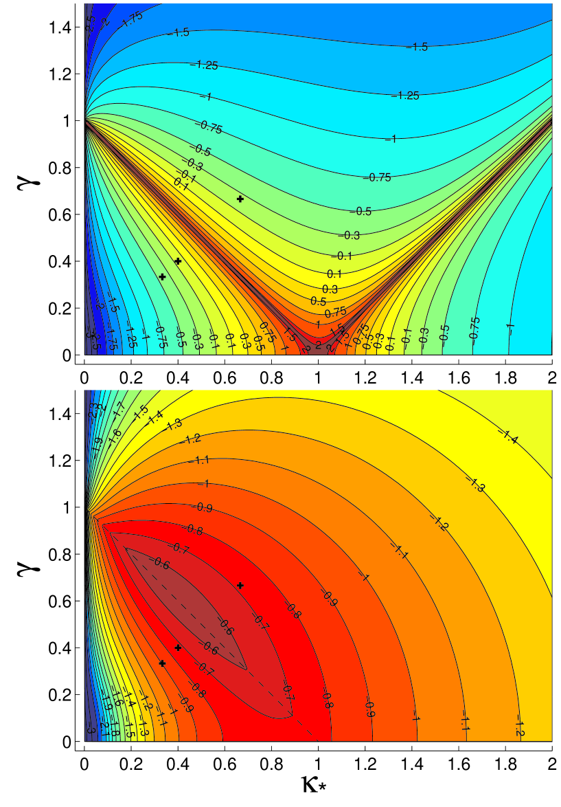
Figure 1.— Contour plots of $\log_{10}(\langle n\rangle)$ (upper panel) and $\log_{10}(\langle n\rangle/\langle\mu\rangle)$ (lower panel) in the $\kappa_{*}-\;\gamma$ plane. The dashed line in the lower panel shows the line of infinite magnification $\gamma=1-\kappa_{*}$ along which there is a “ridge” in $\langle n\rangle/\langle\mu\rangle$, while the three plus symbols in both panels mark the values used in our three simulations: $\kappa_{*}=\gamma=0.333,\,0.400,\,0.666$.

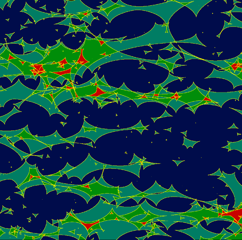
Figure 2.— A map of the number of extra micro-image pairs $n$ in the source plane, for the simulation with $\gamma=\kappa_{*}=0.666$. The regions in dark blue, turquoise, green, red and orange, correspond to $n=0,\,1,\,2,\,3$ and $4$, respectively. The yellow lines represent the caustics, while regions for which $n$ could not be determined are in black.

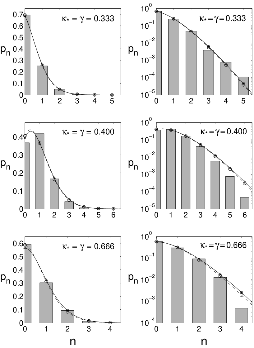
Figure 3.— The bars show the probability $p_{n}$ of having $n$ extra image pairs, calculated from our simulations ($\kappa_{*}=\gamma=0.333,\,0.400,\,0.666$), using equation (9). The lines correspond to a Poisson distribution [equation (13)] where the solid line is for the analytical (theoretical) mean value $\langle n\rangle$, and the dashed line is for the mean value from the simulation $\langle n\rangle_{\rm sim}$, calculated according to equation (10). The theoretical values of $p_{n}$ for integer values of $n$ are shown by the asterisk and circle symbols. The panels on the left (right) column are linear (logarithmic) representations of $p_{n}$.

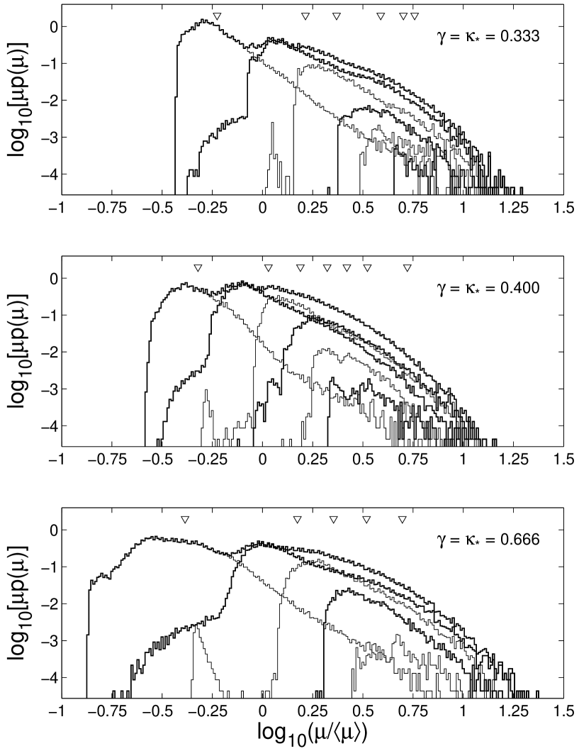
Figure 4.— A log-log plot of the magnification distribution for the macro-image $\mu p(\mu)$ (uppermost line), for our simulations, and its decomposition, $\mu p_{n}(\mu)$, to the contributions from regions with different numbers of extra image pairs, $n$. The alternating thin and thick solid lines, from left to right, are for $n=0$ through $6$. The inverted triangles represent the average magnification from regions with $n$ extra image pairs, $\langle\mu\rangle_{n}$.

References

- Burud et al. (1998) Burud, I., Stabell, R., Magain, P., et al. 1998, A&A, 339, 701
- Chang & Refsdal (1979) Chang, K., & Refsdal, S. 1979, Nature, 282, 561
- Chiba (2002) Chiba, M. 2002, ApJ, 565, 17
- Corrigan et al. (1991) Corrigan, R.T., et al. 1991, AJ, 102, 34
- Dalal & Kochanek (2002) Dalal, N., & Kochanek, C.S. 2002, ApJ, 572, 25
- Gaudi, Granot & Loeb (2001) Gaudi, B.S., Granot, J., & Loeb, A. 2001, 561, 178
- Garnavich, Loeb & Stanek (2000) Garnavich, P.M., Loeb, A., & Stanek, K.Z. 2000, ApJ, 544, L11
- Merino, Wisotzki & Wambsganss (2002) Gil-Merino, R., Wisotzki, L., & Wambsganss, J. 2002, A&A, 381, 428
- Hewitt et al. (1992) Hewitt, J.N., Turner, E.L., Lawrence, C.R., Schneider, D.P, Brody, J.P. 1992, AJ, 104, 968
- Inada et al. (2002) Inada, N., et al. 2002, submitted to ApJ
- Irwin et al. (1989) Irwin, M.J., Webster, R.L., Hewett, P.C., Corrigan, R.T., Jedrzejewski, R.I. 1989, AJ, 98, 1989
- Jackson, Xanthopoulos & Browne (2000) Jackson, N.J., Xanthopoulos, E., & Browne, I.W.A. 2000, MNRAS, 311, 389
- Katz et al. (1986) Katz, N., Balbus, S., & Paczyński, B. 1986, ApJ, 306, 2
- Koopmans & Wambsganss (2001) Koopmans, L.V.E., & Wambsganss, J. 2001, MNRAS, 325, 1317
- Lawrence et al. (1995) Lawrence, C.R., Elston, R., Januzi, B.T., & Turner, E.L. 1995, AJ, 110, 2570
- Lewis & Irwin (1995) Lewis, G.F., & Irwin M.J. 1995, MNRAS, 276, 103
- Lewis & Irwin (1996) Lewis, G.F., & Irwin M.J. 1996, MNRAS, 283, 225
- Lewis et al. (1998) Lewis, G.F., Irwin, M.J., Hewett, P.C., & Foltz, C.B. 1998, MNRAS, 295, 573
- Mao & Scneider (1998) Mao, S., & Scneider, P. 1998, MNRAS, 295, 587
- Metcalf & Madau (2001) Metcalf, R.B, & Madau, P. 2001, ApJ, 563, 9