Pairwise velocity dispersion of galaxies at high redshift: theoretical predictions

Abstract

We investigate the feasibility of determining the pairwise velocity dispersion (PVD) for Lyman Break Galaxies(LBGs), and of using this quantity as a discriminator among theoretical models. We find that different schemes of galaxy formation lead to significant changes of the PVD. We propose a simple phenomenological model for the formation of Lyman break galaxies, determined by the formation interval parameter $\Delta_{z}$ and the halo mass threshold $M_{h}$. With a reasonable choice for these two parameters, our model predicts an occupation number distribution of galaxies in halos which agrees very well with the predictions of semi-analytical models. We also consider a range of galaxy formation models by adjusting the two model parameters. We find that model LBGs can have the same Two Point Correlation Function (TPCF) over the range of observable separations even though the cosmology and/or galaxy formation model are different. Moreover, with similar galaxy formation models, different currently popular cosmologies can result in both the same TPCF and the same PVD. However, with the same cosmology, different galaxy formation models may show quite different PVDs even though the TPCF is the same. Our test with mock samples shows furthermore that one can discriminate among such models already with currently available observational samples (if the measurement error of the redshift is negligible) which have a typical error of $80\,{\rm{km\,s^{-1}}}$. The error will be reduced by a factor of 2 if the samples are increased four times. We also show that an erroneous assumption about the geometry of the universe and different infall models only slightly change the results. Therefore the PVD will become another promising statistic to test galaxy formation models with redshift samples of LBGs.

1 Introduction

The Lyman break technique developed by Steidel and his coworkers has opened a window to uncover high-redshift galaxies at redshift $z\approx 3$ based on ground-based photometric observations only (Steidel et al. 1996; Steidel et al. 1999). The technique has proved to be very efficient, since most of the candidates identified with photometric colors have been confirmed as high-redshift galaxies in subsequent spectroscopic observations. About 1000 Lyman-break galaxies with redshifts have already been compiled by Steidel’s group. The sample of high-redshift galaxies is likely to be enlarged significantly in the next years with more 10-meter telescopes being used in the observations (e.g. Ouchi et al. 2001).

Lyman-break galaxies have been found to be strongly clustered. The correlation length of the galaxies is $3$ to $6\,h^{-1}{\rm{Mpc}}$ in comoving coordinates, similar to that of local normal galaxies (Steidel et al. 1998; Adelberger et al. 1998; Giavalisco et al. 1998; Connolly, Szalay & Brunner 1998; Arnouts et al.1999; Adelberger & Steidel 2000; Giavalisco & Dickinson 2001, hereafter GD01). The strong clustering is generally expected in cold dark matter (CDM) models if the galaxies are hosted by massive halos with mass $M\lower 2.15277pt\hbox{$\;\buildrel>\over{\sim}\;$}5\times 10^{11}\,h^{-1}{M_{\odot}}$ (Mo & Fukugita 1996; Steidel et al. 1998; Jing & Suto 1998; Giavalisco et al. 1998; Adelberger et al. 1998; Connolly, Szalay & Brunner 1998). Combined with other observations of Lyman Break galaxies, such as the star formation rate, kinematics, metal abundances, it is hoped that the clustering properties of the high-redshift galaxies can set significant constraints on galaxy formation models.

Current theoretical models (e.g. the standard CDM model and the $\lambda$-dominated CDM model) have been fine-tuned to fit the local observations. The degeneracy found in the model parameters might be broken with the help of observations at high redshift, like those of Lyman-break galaxies.

The clustering of Lyman-break galaxies is found to be consistent with the predictions of most currently interesting models, partly because these models have been tested by other observations and partly because LBGs with different host halo mass can exhibit the same clustering property as long as galaxy formation recipes are tuned correspondingly. In a recent study by Wechsler et al. (2001, hereafter W01), five scenarios were examined for associating dark matter halos in the standard LCDM model with Lyman-break galaxies, and the clustering length of the model galaxies was compared with the observations of Adelberger & Steidel (2000). They conclude that the strong clustering of Lyman-break galaxies can generally be reproduced in different cosmogonic models (including the mixed dark matter model) by adjusting the galaxy formation recipes (e.g. introducing plausible physical processes like starbursts, but in an average way by adjusting various global parameters). Although the host halo mass is rather different in different cosmogonic models, these differences could not be used to discriminate among models, mainly because reliable determinations of the mass of halos hosting Lyman break galaxies are lacking. Early spectroscopic observations indicate that the LBGs are hosted by massive halos (Steidel et al. 1996), but recent observations reveal that the disk rotation within Lyman-break galaxies could be much slower than was thought before (Pettini et al. 2001). Thus between models of different hosting galaxies a choice could not be made yet.

The pairwise velocity dispersion (PVD) of galaxies, which probes the dark matter potential, could provide information about the dark matter distribution which is independent of and complementary to the spatial distribution of galaxies (e.g. the two-point correlation function). The PVD has already been widely applied to the local redshift surveys of galaxies, and has yielded very valuable information about the dynamics of local galaxies which has been widely taken as important input for the cosmological models. The PVD of galaxies determined (Davis & Peebles 1983) from the first wide angle redshift survey of galaxies, the Center for Astrophysics (CfA) redshift survey, was one principal reason to argue for biased galaxy formation, i.e. for a difference in the distribution of the galaxies and the dark matter particles. This survey was later found to be too small for robustly measuring the PVD (Mo et al. 1993). The publicly available Las Campanas Redshift survey of galaxies is about ten times larger than the CfA, and Jing, Mo, & Börner(1998, hereafter JMB98) have measured the PVD for this survey. The accurate PVD measurement of the LCRS survey not only constrains the $\beta$ parameter of the CDM models to around $0.4$ (where $\beta=\Omega_{0}^{0.6}\sigma_{8}$, $\Omega_{0}$ is the current density parameter and $\sigma_{8}$ the rms linear density contrast within a sphere of $8\,h^{-1}{\rm{Mpc}}$), but also suggests an anti-bias for the local galaxy distribution on very small scales. The statistical results of JMB98 are confirmed by a recent analysis of the early data release of the Sloan Digital Sky Survey (Zehavi et al. 2002).

The PVD could also be a very important observable quantity for high redshift galaxies, when redshift surveys, like those of the Lyman Break galaxies and the DEEP2 survey become available. The local observations, like the cluster abundance, the PVD of galaxies, and the peculiar velocity field of galaxies, require that the $\beta$ is around $0.4\sim 0.5$ almost independently of whether the cosmos is open, flat or dominated by vacuum energy. The local degeneracy may be broken by the PVD observation at high redshift. Because the density fluctuation grows quite differently in different cosmological models, the $\beta$ value is very different at high redshifts in these models. The $\beta$ value is much smaller in the SCDM than that in the LCDM model, as is the pairwise velocity dispersion of the dark matter. Since the Lyman-break galaxies are known from their high spatial correlation to be a biased tracer of the dark matter they do not uniformly sample the dark matter distribution, so the pairwise velocity dispersion of LBGs could differ significantly from that of the dark matter. Thus a measurement of their PVD may be useful to put constraints on the galaxy formation models, but it is unknown if it is feasible to measure this important quantity with observations available now or in the near future.

In this paper, we investigate this important issue within two CDM models: the SCDM and LCDM. We will attempt to address the following four questions: 1) how does the bias of the LBGs relative to the dark matter show up in the PVD; 2) how does the PVD of Lyman break galaxies depend on the cosmological model; 3) how does the PVD of LBGs depend on the recipes for galaxy formation; 4) how accurately can one measure the PVD of Lyman break galaxies with currently available samples and with samples available in the near future.

Although this work is focused on the Lyman Break galaxies, the approach is readily extended to other high-redshift galaxy surveys, like the DEEP2 survey, where an important goal is the measurement of the PVD of galaxies at redshift about one (Coil et al. 2001). As galaxies at $z=1$ may be more closely connected to the galaxies at $z=0$, the PVD study of the DEEP2 survey can probably yield interesting constraints on theoretical models.

The paper is arranged as follows: We will use a plausible phenomenological model to identify Lyman break galaxies from high-resolution N-body simulations, as described in §2. The model predicts the occupation number of galaxies within halos. This agrees very well with the prediction of a physically motivated semi-analytical model of galaxy formation. Because the PVD and the correlation function of galaxies mainly depend on the occupation number of galaxies in halos, we believe that our results represent the prediction of a class of physically motivated galaxy formation models. We also investigate how the PVD depends on formation models of galaxies and the difference in PVD between galaxies and dark matter. We will discuss the possibility of discriminating between cosmological models with the PVD measurement. In §3, we consider a set of mock samples generated according to the observational strategy of Steidel et al. (1998), and assess the accuracy of the PVD measurement with currently available Lyman break galaxy samples and with samples available in the near future. With these mock samples we will also discuss how the measurement depends on the assumption of the world model. Our results will be further discussed in the final section §4.

2 Identification of LBGs in CDM simulations and their clustering properties

We consider two typical Cold Dark Matter (CDM) models. One is the (no longer) standard CDM model (SCDM) with a density parameter $\Omega_{0}=1$, and the other is a flat CDM model with $\Omega_{0}=0.3$ and a vacuum energy density $\lambda_{0}=0.7$ (LCDM). These CDM models are completely fixed with regard to the dark matter clustering once the linear density power spectrum is chosen. The linear transfer function of Bardeen et al. (1986) together with a primordial Harrison-Zel’dovich spectrum is taken for the models. The linear power spectrum is then fixed by the shape parameter $\Gamma=\Omega_{0}h$ and the amplitude $\sigma_{8}$ (the rms top-hat density fluctuation on radius $8\,h^{-1}{\rm{Mpc}}$). The values of ($\Gamma$, $\sigma_{8}$) are (0.5, 0.62) for SCDM and (0.2, 1) for LCDM. We note that all the parameters taken for the LCDM are consistent with observations, and this model now indeed can be viewed as the standard CDM model.

The simulations were generated on the Fujitsu VPP300/16R supercomputer at the National Astronomical Observatory of Japan. Each simulation is performed with a vectorized $\rm P^{3}M$ code using $256^{3}$ ($\approx 17$ million) particles. The box size is $100\,h^{-1}{\rm{Mpc}}$ and the effective force resolution $\eta\approx 0.039\,h^{-1}{\rm{Mpc}}$. These CDM simulations were used by Jing & Suto (1998) to study the constraints on cosmological models derived from the high concentration of the Lyman Break galaxies at redshift $z\approx 3$ discovered by Steidel et al. (1998).They were also used to study the clustering of dark matter halos (Jing 1998) and many other interesting problems.

Galaxies, including Lyman break galaxies, are believed to form within dark matter halos. We find halos in the simulations using the Friends-of-Friends (FOF) method with the bonding length equal to 0.2 times the mean particle separation. Between redshift 2 and 4, each of our simulations has seven outputs with time intervals $\Delta\ln(1+z)=0.08$, and all halos with more than 10 FOF members have been identified at each epoch.

It is, however, highly non-trivial to relate galaxies to the identified halos in a quantitative way. In early studies the strong clustering of the LBGs was implemented by a one-to-one correspondence between a galaxy and a halo above certain mass threshold. This massive halo model (Mo & Fukugita 1996; Adelberger et al. 1998; Wechsler et al. 1998; Jing & Suto 1998; Bagla 1998; Coles et al. 1998; Moscardini et al. 1998; Arnouts et al. 1999), though extremely simplified, provided an explanation at least in a qualitative manner, of most of the observed properties of LBGs, especially their strong clustering. Semi-analytical methods (Cole et al. 1994; Baugh et al. 1998; Katz et al. 1999; Somerville et al. 2000; Weinberg et al. 2000; W01), which allow to take physical processes such as gas cooling, halo and galaxy merging, star formation and its feedback, into account in a more realistic way, have been employed to determine the relation between galaxies and halos. If galaxies form quiescently from the cooled gas within halos, these galaxies lie essentially in halos with a narrow range of masses. Thus the quiescent model is actually very similar to the massive halo model, although in the former model, the lower halo mass cutoff is not sharp and the most massive halos which are more massive than the typical halos can host more than one galaxy. In these aspects, the quiescent model is believed to be more realistic than the massive halo model. On the other hand, the quiescent model has its own uncertainties, e.g. star formation law of cold gas at high redshift can be chosen in a variety of ways. Also the influence of galaxy collisions on star formation is uncertain.

In this paper we present a simple model for relating Lyman-break galaxies to halos. We assume that LBGs seen at redshift $z_{o}$ formed within FOF halos above a certain mass $M_{h}$ at an earlier time $z_{f}$ with a one-to-one correspondence. The galaxy is tagged to the particle of the minimum of the gravitational potential within the halo. The position and velocity of the galaxy at redshift $z_{o}$ are derived from those of the minimum-potential particles. Thus we have equivalently assumed that no merger happened to galaxies between redshift $z_{o}$ and redshift $z_{f}$. We use $\Delta_{z}\equiv\ln(1+z_{f})-\ln(1+z_{o})$ as a parameter. The number density of LBG peaks at $z_{o}\approx 3.0$, and the observations of Steidel et al. (1996) indicate that stars of Lyman Break galaxies are roughly one Gyr old, that is $\Delta_{z}\approx 0.32$ for the LCDM model. Compared with the massive halo model, we allow very massive halos to host more than one galaxy. This property is important for studying the velocity dispersion of galaxies, since it has been known that the velocity dispersion is sensitive to the presence of groups or clusters of galaxies.

Once this parameter has been fixed, we can determine the parameter $M_{h}$ based on the facts that the comoving density of galaxies at redshift $z=3$ should be above $1.0\times 10^{-3}h^{3}\,{\rm Mpc}^{-3}$, and that the correlation length is about $5.0\,h^{-1}{\rm{Mpc}}$ for the LCDM universe ($4.0\times 10^{-3}h^{3}\,{\rm Mpc}^{-3}$ and $3.1\,h^{-1}{\rm{Mpc}}$ for the SCDM model) (GD01). We use the observed density as the lower limit, because the samples of LBGs may not have included all the galaxies in the survey volumes (GD01). The two-point correlation function (TPCF) of the model LBGs is presented in Figure 1 for several choices of $M_{h}$. The spatial distribution of the model LBGs is positively biased, and the bias increases with the mass parameter $M_{h}$ as expected. Comparing with the observed values of the clustering length (GD01), we find that $M_{h}=2.0\times 10^{11}\,h^{-1}{M_{\odot}}$ and $1.7\times 10^{11}\,h^{-1}{M_{\odot}}$ are suitable choices for the LCDM model and the SCDM model, respectively. These models are LCDM40 and SCDM10 in Table 1. For these $M_{h}$ values, the spatial number densities of model LBGs are about $7$ and $14\times 10^{-3}h^{3}\,{\rm Mpc}^{-3}$ respectively, somewhat larger than the observed density for LBGs brighter than $25.5$ in the red band (Steidel et al. 1999; Adelberger & Steidel 2000; GD01), and so meets the above density criterion. We have examined the LCDM model further by considering the occupation number distribution of galaxies in halos. Figure 2 shows this quantity together with the semi-analytical predictions of W01 for this cosmological model. The mean occupation number from our prescription is very close to the predictions of their Constant Efficiency Quiescent model and Accelerated Quiescent model, but slightly higher than the prediction of their Collisional Starburst for massive haloes. Their work, which carefully compared the clustering on small scales in models and in observations of Lyman break galaxies, strongly favors the first two models, implying that our simple prescription has already caught the main physical processes related to the formation of LGBs. For the purpose of this paper which is to examine the pairwise velocity dispersion of LBGs, our recipe for identifying LBGs in the simulations should be adequate , since the statistics examined in this paper are mainly determined by the occupation number distribution (JMB98).

The pairwise velocity dispersion of the model LBGs is presented in Figure 3, together with that of the dark matter for a comparison. The PVDs of the model LBGs for the range of halo mass $M_{h}$ considered are all higher than the PVDs of the dark matter, and they increase with the halo mass $M_{h}$. A similar behavior is seen in the TPCF. This result can be easily understood, since the LBGs in the model are located in massive halos. Although the dark matter has a much higher PVD in the LCDM model than in the SCDM model, the LBGs with $M_{h}\approx 2\times 10^{11}\,h^{-1}{M_{\odot}}$ have a very similar PVD in both cosmological models. This indicates that the local degeneracy of the two cosmological models may not be broken with the measurements of the two-point CF and the pairwise velocity dispersion for LBGs. It also must be admitted that there are big uncertainties still in our current knowledge of how LBGs have formed. Previous work including the semi-analytical work of W01 to which our simple model has been compared, indicates that LBGs are formed within massive halos. But some recent observations and theoretical models indicate that LBGs are preferentially formed within less massive halos (Pettini et al. 2001; Shu, Mao, & Mo 2001). It would be important to find observations to discriminate between these different theoretical approaches. This is exactly one of our initial motivations to consider the PVD for LBGs.

Different formation models will predict different Occupation number Distributions of galaxies within Halos (ODH). Different ODHs can be produced in our model by adjusting the two model parameters $M_{h}$ and $\Delta_{z}$. For a given $\Delta_{z}$, LBGs are preferentially within massive halos for larger $M_{h}$. For a given $M_{h}$, LBGs are preferentially within small halos for a small $\Delta_{z}$, because fewer mergers happened within a shorter time period and massive halos have fewer LBGs than when $\Delta_{z}$ is larger. These points can be clearly seen from Figure 4 where we plotted the ODH for several models with different combinations of $M_{h}$ and $\Delta_{z}$ listed in Table 1.

Table 1:

	Galaxy Ident.		3-d Density		3-d TPCF		Mock TPCF
Model	$\Delta_{z}$	$M_{h}$	$z=3.18$	$z=2.86$	$z=3.18$	$z=2.86$	$r_{0}[h^{-1}\rm Mpc]$ $\gamma$
LCDM13	0.56	0.66	0.0121	0.0175	5.60 1.67	5.15 1.66	$5.07\pm 0.45$ $1.75\pm 0.14$
LCDM40	0.32	2.04	0.0059	0.0078	5.52 1.68	5.14 1.66	$5.12\pm 0.45$ $1.71\pm 0.12$
LCDM95	0.08	4.84	0.0038	0.0048	5.28 1.60	4.82 1.62	$4.80\pm 0.43$ $1.64\pm 0.15$
SCDM10	0.32	1.70	0.0119	0.0187	3.24 1.80	3.00 1.75	$2.99\pm 0.25$ $1.88\pm 0.14$
SCDM25	0.08	4.25	0.0080	0.0116	3.33 1.72	3.02 1.70

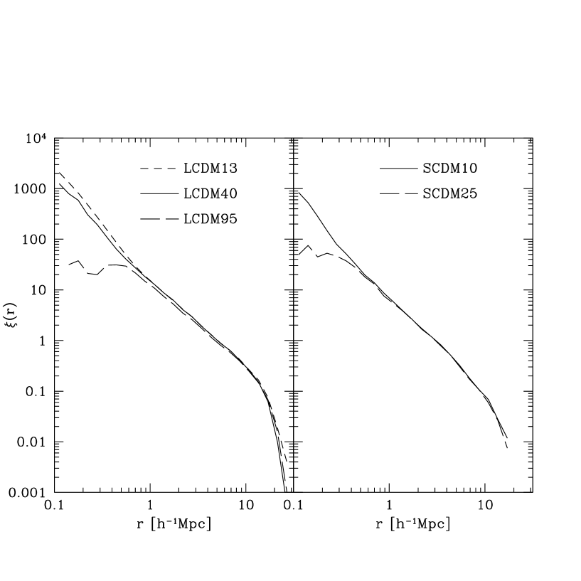
Figure 5: Real space two-point CF of LBGs at $z=2.86$ for different models listed in Table 1.

In Figures 5 and 6, we plot the TPCF and velocity dispersion for the models listed in Table 1. By our design, all these models have very similar angular TPCFs, though their ODHs and cosmogony are quite different, indicating that these models cannot be distinguished by the observation of the TPCF alone. However, the PVDs are significantly different for different ODHs. The key question now is, whether observational catalogues of LBGs already available or available in the near future are large enough for this purpose. We will address this issue in the next section, where we will examine the feasibility of measuring the PVD of LBGs using mock samples.

3 Accuracy of measuring PVD for LBGs

Our simulations have 7 outputs between $z=2$ and $z=4$. We generate our mock samples by combining LBGs at these outputs with periodic replications. We will mainly use the LBGs with $M_{h}\approx 2.0\times 10^{11}\,h^{-1}{M_{\odot}}$ and $\Delta_{z}=0.32$ for the analysis of this section, since we think that this sample is sufficient for our purpose of examining the PVD measurement error. The peculiar velocity is taken into account properly when computing the redshift for each mock galaxy. The mock samples are generated in pencil beams with a fixed sky area of $9^{\prime}\times 18^{\prime}$. The galaxies are further randomly culled according to the redshift selection function (Figure 7). The selection function is obtained from a spline-interpolation of the redshift distribution histogram presented by Pettini et al.(1997) and is normalized so that the galaxy surface density is 0.8 per square arcminute as observed by GD01. A total of 1000 of such beams has been produced in randomly selected directions (all cross correlations between such beams are neglected here). Our method of generating the mock samples is essentially the same as that of Jing & Suto (1998).

When measuring the TPCF and PVD for the mock samples, we first assume a world model and then compute comoving coordinates for each mock galaxy in redshift space. Given a pair of galaxies with comoving coordinates ${\bf q}_{1}$ and ${\bf q}_{2}$, we define ${\bf s}={\bf q}_{1}-{\bf q}_{2}$ and ${\bf l}=\frac{1}{2}({\bf q}_{1}+{\bf q}_{2})$. Then for a flat universe and under the small angle approximation, the separations along ($\pi$) and perpendicular ($r_{p}$) to the line of sight are,

$$\pi={\bf s\cdot l/|l|},$$ (1)

$$r_{p}^{2}={\bf s\cdot s}-\pi^{2}.$$ (2)

We estimate the redshift-space two-point correlation function $\xi_{z}(r_{p},\pi)$ by

$$\xi_{z}(r_{p},\pi)=\frac{4RR(r_{p},\pi)DD(r_{p},\pi)}{[DR(r_{p},\pi)]^{2}}-1,$$ (3)

where $DD(r_{p},\pi)$, $DR(r_{p},\pi)$ and $RR(r_{p},\pi)$ refer to the counts of data-data, data-random and random-random pairs with separations $\pi$ and $r_{p}$ respectively (Hamilton 1993). A random sample, which contains 200,000 points, is generated in the same way as the mock samples, except that the points are randomly distributed in redshift space before the selection effects are applied.

The projected two-point correlation function $w(r_{p})$ is estimated from

$$w(r_{p})=\int\limits_{0}^{\infty}{\xi_{z}(r_{p},\pi)\,d\pi}=\sum_{i}\xi_{z}(r_{p},\pi_{i})\Delta\pi_{i},$$ (4)

where $\xi_{z}(r_{p},\pi)$ is measured by equation (3). In order to examine the dependence of the measurement accuracy on the sample size, we combine pencil beams into groups and calculate the mean and standard variance of $w(r_{p})$ among the beam groups. Every beam group may have 10, 20 or 50 beams, for the currently available data contain already 10 beams and a sample as large as 50 beams is expected to be available in the near future. The projected two-point correlation function for one randomly selected beam group is presented in each panel of Figure 8. Triangles are the mean among different beams in the group, and error bars show the corresponding $1\sigma$ scatter among the beams divided by the square root of the beam number in the group. Different assumptions about the world model lead to a shift in the amplitude because of the different world geometries.

The projected function $w(r_{p})$ is simply related to the real space TPCF as

$$w(r_{p})=\int\limits_{0}^{\infty}{\xi(\sqrt{r_{p}^{2}+y^{2}})\,dy}.$$ (5)

Assuming a power-law for the two point correlation function $\xi$

$$\xi(r)=(r_{0}/r)^{\gamma},$$ (6)

we can find $\xi(r)$ through a fit of Eq.(5) to the observed $w(r_{p})$. In practice, an upper limit $\pi_{u}$ must be imposed on the integral variables of Eq.(4) and Eq.(5). We will use $\pi_{u}=17.9h^{-1}{\rm Mpc}$ when a low density world model is assumed for calculating the distance and $10.0h^{-1}{\rm Mpc}$ when the Einstein de-Sitter world model is assumed. The power law fitting works well for the projected function $w(r_{p})$ (Figure 8), and we also found that the fitted result describes the 3-d TPCF very well at $0.5\lower 2.15277pt\hbox{$\;\buildrel<\over{\sim}\;$}r\lower 2.15277pt\hbox{$\;\buildrel<\over{\sim}\;$}20\,h^{-1}{\rm{Mpc}}$ (see Table 1). The fitting results are quite robust to a reasonable change in $\pi_{u}$: a $50\%$ increase or decrease in $\pi_{u}$ does not change the results much (less than $3\%$ for both $r_{0}$ and $\gamma$).

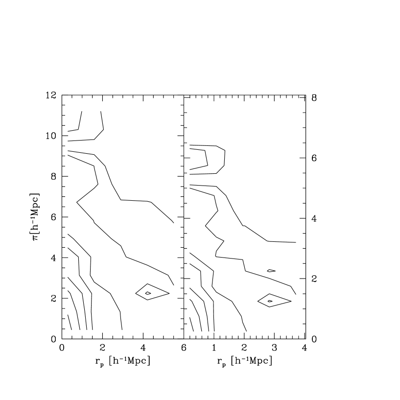
Figure 9: Contours of the redshift space two-point correlation function for one randomly selected 50-beam LCDM40 group. The left panel shows the results with the correct cosmology assumed, while the right panel is for an Einstein-de Sitter Universe.

The pairwise velocity dispersion (PVD) for galaxies is measured in observations by comparing the redshift space two-point correlation function $\xi_{z}(r_{p},\pi)$ along and perpendicular to the line-of-sight. An example of this quantity, which is measured from a randomly selected 50-beam group of LCDM40, is shown in Figure 9. In the left hand panel, the cosmological parameters assumed for calculating the comoving distance are the same as those of the model itself, while in the right panel an Einstein-de Sitter Universe is assumed when estimating the distance. One can find that in both cases the maps are distorted similarly on small scales. Assuming the wrong cosmology introduces a compression factor of 1.2 along the direction of $\pi$, but this effect cannot be separated from the velocity dispersion (see below) so it cannot be used to measure the world geometry (cf. Matsubara & Suto 1996).

Temporarily let the effect of a possible cosmological geometry distortion be absorbed into the PVD measurement. The PVD of galaxies is measured by modeling the redshift distortion in the observed redshift space correlation function $\xi_{z}(r_{p},\pi)$. Following Peebles(1980), Fisher et al. (1994) and JMB98, we assume:

$$1+\xi_{z}(r_{p},\pi)=\int{f(v_{12})\{1+\xi[\sqrt{r_{p}^{2}+(\pi-v_{12}(1+z)/H(z))^{2}}]\}dv_{12}},$$ (7)

where $H(z)$ is the Hubble constant at redshift $z$. For the real space TPCF $\xi(r)$, the power-law fit of the data is used, and for $f(v_{12})$, the distribution function of the relative velocity along the line of sight, we adopt an exponential form as follows which is supported by observations (Davis & Peebles 1983; Fisher et al. 1994), theoretical models(Diaferio & Geller 1996; Sheth 1996; Seto & Yokoyama 1998) and direct simulations (Efstathiou et al. 1988; Magira, Jing & Suto 1999):

$$f(v_{12})=\frac{1}{\sqrt{2}\sigma_{12}}{\rm exp}(-\frac{\sqrt{2}}{\sigma_{12}}|v_{12}-\overline{v_{12}}|),$$ (8)

where $\overline{v_{12}}$ is the mean and $\sigma_{12}$ the dispersion of the one-dimensional pairwise peculiar velocities. Here we use two infall models for reconstructing the PVD from the mock samples. In both models,

$$\overline{v_{12}}=-y\overline{V_{12}}(r)/r,$$ (9)

where $y$ is the separation along the line of sight in real space and $\overline{V_{12}}$ is the mean relative velocity of two galaxies with a separation $r$. The velocity difference $\overline{V_{12}}$ can be directly measured from the simulations, but hardly in observations. To see the sensitivity of the results to this quantity, we adopt two types of $\overline{V_{12}}$ for equation (8): one is called the real infall model which is the quantity directly measured from corresponding simulation data of LBGs, and the other is called the average infall model which is an average for this quantity from LCDM40 and SCDM10.

When estimating $\sigma_{12}$ with the least square fitting method (cf. JMB98), we measure the average of $\xi_{z}(r_{p},\pi)$ over beams in the group under consideration and use the inverse of the standard error of the averaged $\xi_{z}(r_{p},\pi)$ as the weight in the least-square fitting. The fitting results are illustrated in Figure 10 for one 50-beam LCDM40 mock sample which indicates that the fitting model works quite satisfactorily. The real space two-point CF $\xi(r)$ (i.e. without a redshift distortion) is plotted for comparison.

The measurement of the PVD from mock samples using the above procedure is compared in Figure 11 with the true PVD directly calculated from simulation. The true PVD is defined as $\langle[{\bf v}_{12}({\bf r})^{2}-\langle{\bf v}_{12}({\bf r})\cdot{\bf\hat{r}}\rangle^{2}]/3\rangle^{1/2}$. The dashed lines are the true PVD obtained at two epochs $z=2.86$ and $3.18$, where the density of observed galaxies (due to the selection effect) is peaked. The points and error bars are the average and standard variance respectively, among the results of 100 ten-beam samples and 20 fifty-beam samples. In the plot, we assumed a correct world model for calculating the comoving distance. At these $r_{p}$, the standard deviation among those 10-beam (50-beam) samples is about $80\,{\rm{km\,s^{-1}}}$ ($35\,{\rm{km\,s^{-1}}}$) which should be the typical error in the real measurement when the observational sample is as large as the mock sample. Variation of $\pi_{u}$ from $13.5$ to $27\,h^{-1}{\rm{Mpc}}$ introduces a shift of the PVD of several $\,{\rm{km\,s^{-1}}}$ at the first three $r_{p}$ and by tens at the last. Therefore the effect of varying $\pi_{u}$ is in general negligible. It has been noted that the PVD measured with the above procedure may differ from that given directly by the 3-D velocities of galaxies (JMB98). For this mock sample, the PVD reconstructed from the redshift distortion agrees very well with that from the 3D velocity, and is also quite robust to a reasonable change of the infall model. So, different galaxy formation models which show a difference of a few hundred $\,{\rm{km\,s^{-1}}}$ in the PVD can be tested with progressively larger samples, as seen from Fig. 6.

Figure 12 shows the predictions for the pairwise velocity dispersion measured from a set of mock samples of LCDM40 (solid lines, filled symbols with error bars) and SCDM10 (dotted lines, open symbols with error bars). Let the observer assume that the cosmology is either that of LCDM or that of SCDM. These world models are quite typical in current research work. The lines in the figure are obtained by assuming a correct world model and the symbols by assuming a wrong world model. Furthermore, we use two types of infall models: left hand panels show the real infall model and right hand panels the average infall model. From the figure, we find: 1) the PVD is the same for LCDM40 and SCDM10 mock smaples at small separations. This is consistent with the result seen in the 3-d PVD of Figure 3, reinforcing that these two models could not be distinguished by the PVD measurement; 2) the typical error is $80\,{\rm{km\,s^{-1}}}$, $60\,{\rm{km\,s^{-1}}}$, and $35\,{\rm{km\,s^{-1}}}$ for the PVD at a separation $r_{p}\approx 1\,h^{-1}{\rm{Mpc}}$ for the beam number 10, 20 and 50 respectively. It is easy to see that the error decreases with the square root of the beam number; 3) assuming the wrong world model can bring about an increase or a reduction of up to $100\,{\rm{km\,s^{-1}}}$ at $r_{p}=5\,h^{-1}{\rm{Mpc}}$. But the effect is smaller for smaller separations, and is negligible for $r_{p}\leq 1\,h^{-1}{\rm{Mpc}}$; 4) the difference of the PVD caused by the difference in the infall models is small, generally less than $20\,{\rm{km\,s^{-1}}}$. Actually, when using PVD to distinguish theoretical models, we compare observed results with those of mock samples rather than with real 3-D PVD due to definition difference, the effects in 3) and 4) will disappear completely.

4 Discussion and conclusions

We have investigated the feasibility of determining the pairwise velocity dispersion for the Lyman Break Galaxies, and of using this quantity as a discriminator among theoretical models. Our central conclusion is that the PVDs change significantly with different schemes of galaxy formation within the same cosmogony model. On the other hand, with similar galaxy formation models, the same two-point correlation function and pairwise velocity dispersion can be obtained for several currently popular cosmogony models. Thus, the PVD of high-redshift objects can be used to set constraints on the way galaxies form (even through cosmogony keeps unknown).

We have proposed a simple phenomenological model for the formation of Lyman break galaxies which is determined by the formation interval parameter $\Delta_{z}$ and the halo mass threshold $M_{h}$. With a reasonable choice for these two parameters, our model predicts an occupation number distribution of galaxies in halos which agrees very well with the predictions of semi-analytical models (W01). This implies that our model incorporates the essential physical processes involved in the formation of the Lyman Break galaxies. Since in our scheme the properties of LBGs are mainly determined by the occupation number distributions of galaxies, we can allow for uncertainties in the current understandings (e.g. the semi-analytical model) of galaxy formation by adjusting the two model parameters. It is likely that the massive halo model and the recent model proposed by Shu et al. (2001) can predict a PVD a few hundred $\,{\rm{km\,s^{-1}}}$ smaller than our fiducial models at the same separation $r_{p}$. Our tests with mock samples show that such models can already be constrained with currently available observed samples (if the measurement error of the redshift is negligible; see discussion below), where the PVD has a typical error of $80\,{\rm{km\,s^{-1}}}$. This error will be reduced by a factor of 2 if the samples are increased four times. Therefore the PVD will become another promising statistic to test galaxy formation models with redshift samples of LBGs.

The determination of the PVD at small separation $r_{p}$ is insensitive to the assumptions about the world model for computing the comoving separations of galaxies. Measuring redshift distortions at small scales therefore cannot be used to measure the cosmological parameters, though the cosmological parameters might be effectively constrained by the distortion measurement on larger scales (Matsubra & Suto 1996; Ballinger et al. 1996).

The typical error of the PVD for a 10-beam sample is $80\,{\rm{km\,s^{-1}}}$ only, and this is really the accuracy one can achieve with currently available redshift samples of LBGs. As Mo et al. (1993) and later other authors (Zurek et al. 1994; Marzke et al. 1995) found, the value of PVD is very sensitive to the presence or absence of rich clusters in a sample, and a redshift sample much larger than the CfA survey which has about 2000 galaxies is needed to achieve an accuracy of $\sim 100\,{\rm{km\,s^{-1}}}$ in the determination of the PVD for local galaxies. Indeed the accuracy of measuring the PVD for the Las Campanas Redshift Survey which contains 25,000 galaxies is $75\,{\rm{km\,s^{-1}}}$ (JMB98), very similar to our expected error for a 10-beam sample of LBGs. The reason is simply that the PVD is better determined at high redshift, because there rich clusters are much rarer, and the effective volume of 10 beams is large enough to include many massive halos formed at that time.

So far we have not taken into account the measurement error in observing the redshift. The measurement error may be treated just like a random motion which can contribute to the measured result of the pairwise peculiar velocity. Thus, in order that the PVD of the LBGs can be measured, the redshift error is required to be much smaller than $400\,{\rm{km\,s^{-1}}}/\sqrt{2}/c\approx 0.001$. Correspondingly, the spectral resolution in the measurement should be better than $7{\rm\stackrel{{\scriptstyle o}}{{A}}}$ at $7000{\rm\stackrel{{\scriptstyle o}}{{A}}}$, if just one line is used. Steidel et al. (1998) measured the redshifts from $\sim 7$ strong absorption features in the rest-frame far-UV and, when possible, the Ly$\alpha$ emission line, so the random error may not be a problem for measuring the PVD. It is also noted that there is a systematic difference between redshifts determined from emission lines and from absorption lines (Steidel et al. 1998; Pettini et al. 2001). This systematic difference should be taken into account, and its effect on the PVD measurement may be reduced if redshifts either from absorption lines or from emission lines only are adopted. Furthermore, with the help of near-IR spectroscopy of some of the high redshift galaxies, which measures the true redshift (Steidel et al. 1998), we can model the distribution of the redshift error, and thus it is possible to lessen its effect by adding one term to the right hand side of Equation (7) to correct the random error.

     

Figure 1: The real space two-point correlation function of galaxies at $z=2.86$ with the same formation time interval ($\Delta_{z}=0.32$), but different mass limits $M_{h}$. For comparison, the TPCF of the dark matter are also shown.

     

Figure 2: Mean galaxy occupation number for different LCDM models. All are normalized to have the same total galaxy number density.

     

Figure 3: The pairwise velocity dispersion of the galaxies in Fig.1, as determined from the 3-D velocity at $z=2.86$.

     

Figure 4: Mean galaxy occupation number for a different combination of the parameters $M_{h}$ and $\Delta_{z}$ (table 1). The mass of SCDM models has been multiplied by a factor of $0.3$ for clarity.

     

     

Figure 6: The pairwise velocity dispersion as determined from the 3-D velocity for different LBG models in Table 1. Left: from up down the lines are for LCDM13, LCDM40 and LCDM95 respectively. Right: from up down the lines are for SCDM10 and SCDM25. The results obtained from LCDM13 (open) and LCDM95 (filled) 50-beam mock samples are also shown, with circles for average infall and triangles for real infall.

     

Figure 7: Redshift selection function of LBGs, normalized to have 0.8 galaxy per square arcminute(see text).

     

Figure 8: The projected two-point correlation function of four randomly selected mock groups (filled triangles). Error bars are $1\sigma$ deviations among different beams in the group divided by the square root of the beam number. The solid line is the best fit with equation (5). In each panel, the upper data and line are results of a cosmological model with the parameters of the LCDM model, while the lower data and line are for an Einstein-de Sitter universe.

     

     

Figure 10: The line of sight two-point correlation function of one 50-beam LCDM40 mock sample (triangles) and the best fitting (solid lines). Error bars are $1\sigma$ deviations among different beams in the group divided by the square root of the beam number. For comparison, the corresponding power-law fits of $\xi(r)$ are also shown as dotted lines.

     

Figure 11: The pairwise velocity dispersions obtained from different mock samples as well as from the 3-D velocity at $z=2.86$ (solid lines) and $3.18$ (dashed lines), with the same galaxy definition correspondingly. The mean value of the PVD for mock samples are shown by triangles (real infall) and circles (average infall), and the $1\sigma$ scatter among different resamplings with real infall by error bars. Open and filled symbols with error bars are for 10-beam and 50-beam samples respectively.

     

Figure 12: The effect of wrong assumption of world model and infall model on the measuring of PVD from mock samples. Solid and dashed lines are those of LCDM40 and SCDM10 in the correct cosmology correspondingly. The filled and open triangles with error bars are those of LCDM40 and SCDM10 respectively, assuming the wrong cosmology. The effect of wrong assumption about world model and infall model on the two galaxy formation model is opposite.

References

- (1) Adelberger, K. L., & Steidel, C. C. 2000, ApJ, 544, 218
- (2) Adelberger, K. L., Steidel, C. C., Giavalisco, M., Dickinson, M., Pettini, M., & Kellogg, M. 1998, ApJ, 505, 18
- (3) Arnouts, S., Cristiani, S., Moscardini, L., Matarrese, S., Lucchin, F., Fontana, A., & Giallongo, E. 1999, MNRAS, 310, 540
- (4) Bagla, J. S. 1998, MNRAS, 297, 251
- (5) Ballinger, W. E., Peacock, J. A., & Heavens, A. F. 1996, MNRAS, 282, 877
- (6) Baugh, C. M., Cole, S., Frenk, C. S., & Lacey, C. G. 1998, ApJ, 498, 504
- (7) Blanton, M., Cen, R., Ostriker, J., Strauss, M., & Tegmark, M. 2000, ApJ, 531, 1
- (8) Bunn, E. F., & White M. 1997, ApJ, 480, 6
- (9) Carroll, S. M., Press, W. J., & Turner, E. L. 1992, ARA&A, 30, 499
- (10) Cole, S., Aragón-Salamanca, A., Frenk, C., Navarro, J., & Zepf, S. 1994, MNRAS, 271, 781
- (11) Coles, P., Lucchin, F., Matarrese, S., & Moscardini, L. 1998, MNRAS, 300, 183
- (12) Connolly, A., Szalay A.S., & Brunner, R.J. 1998, ApJ, 499, L125
- (13) Davis M., & Peebles P.J.E. 1983, ApJ, 267, 465
- (14) Diaferio A., & Geller M.J. 1996, ApJ, 467, 19
- (15) Fisher K.B., Davis M., Strauss M.A., Yahil A., & Huchra J.P. 1994, MNRAS, 267, 927
- (16) Giavalisco, M. & Dickinson, M. E. 2001, ApJ, 550, 177 (GD01)
- (17) Giavalisco, M., Steidel, C. C., Adelberger, K. L., Dickinson, M. E., Pettini, M., & Kellogg, M. 1998, ApJ, 503, 543, (G98)
- (18) Governato, F., Baugh, C. M., Frenk, C. S., Cole, S., Lacey, C. G., Quinn, T., & Stadel, J. 1998, Nature, 392, 359
- (19) Hamilton A.J.S. 1993, ApJ, 417, 19
- (20) Jing, Y.P. 1998, ApJ, 503, L9
- (21) Jing, Y.P., Mo, H.J., & Börner, G. 1998, ApJ, 494, 1 (JMB98)
- (22) Jing, Y. P. & Suto, Y. 1998, ApJ, 494, L5
- (23) Katz, N., Hernquist, L., & Weinberg, D. H. 1999, ApJ, 523, 463
- (24) Kolb, E., & Turner, M. 1990, The Early Universe. Addison Wesley, Redwood City, California
- (25) Lacey, C. & Cole, S. 1993, MNRAS, 262, 627
- (26) Madau, P., Ferguson, H., Dickinson, M., Giavalisco, M., Steidel, C., & Fruchter, A. 1996, MNRAS, 283, 1388
- Marzke et al. (1995) Marzke, R. O., Geller, M. J., da Costa, L. N. & Huchra, J. P. 1995, AJ, 110, 477
- (28) Matsubara, T. & Suto, Y. 1996, ApJ, 470, L1
- (29) Mo, H. J. & Fukugita, M. 1996, ApJ, 467, L9
- (30) Mo H.J., Jing Y.P., Börner G. 1993, MNRAS, 264, 825
- (31) Moscardini, L., Coles, P., Lucchin, F., & Matarrese, S. 1998, MNRAS, 299, 95
- (32) Ouchi, M., Shimasaku, K., Okamura, S., et al. 2001, ApJ, 558, L83
- (33) Peacock, J. A., & Dodds, S. J. 1994, MNRAS, 267, 1020
- (34) Peebles, P. J. E. 1980, The Large-Scale Structure of the Universe (Princeton University Press)
- (35) Pettini, M., Shapley, A. E., Steidel, C. C., Cuby, J. G., Dickinson, M., Moorwood, A. F. M., Adelberger, K. L., & Giavalisco, M. 2001, ApJ, 554, 981
- (36) Seto, N., & Yokoyama, J.I. 1998, ApJ, 492, 421
- (37) Sheth, R. 1996, MNRAS, 279, 1310
- (38) Shu, C., Mao, S., & Mo, H. 2001, MNRAS, 327, 895S
- (39) Somerville, R. S., Primack, J. R., & Faber, S. M. 2001, MNRAS, 320, 504
- (40) Steidel, C., Adelberger, K., Dickinson, M., Giavalisco, M., Pettini, M., & Kellogg, M. 1998, ApJ, 492, 428
- (41) Steidel, C., Adelberger, K., Giavalisco, M., Dickinson, M., & Pettini, M. 1999, ApJ, 519, 1
- (42) Steidel, C., Giavalisco, M., Dickinson, M., & Adelberger, K. 1996, AJ, 112, 352
- (43) Steidel, C. & Hamilton, D. 1992, AJ, 104, 941
- (44) Wechsler, R. H., Gross, M. A. K., Primack, J. R., Blumenthal, G. R., & Dekel, A. 1998, ApJ, 506, 19
- (45) Wechsler, R., Somerville, R., Bullock, J., Kolatt, T., Primack, J., Blumenthal, G., & Dekel, A. 2001, ApJ, 554, 85 (W01)
- (46) Weinberg, D., Hernquist, L., & Katz, N. 2002, ApJ, 571, 15
- (47) Zehavi, I., Blanton, M., Frieman, J., et al. 2002, ApJ, 571, 172
- Zurek et al. (1994) Zurek, W. H., Quinn, P. J., Salmon, J. K. & Warren, M. S. 1994, ApJ, 431, 559