Causal perturbation theory in general FRW cosmologies II: superhorizon behaviour and initial conditions

G. Amery1 Electronic address: G.Amery @ damtp.cam.ac.uk    and E.P.S. Shellard1 Electronic address: E.P.S.Shellard @ damtp.cam.ac.uk 1 Department of Applied Mathematics and Theoretical Physics
Centre for Mathematical Sciences, University of Cambridge
Wilberforce Road, Cambridge CB3 0WA, U.K.
Abstract

We describe how causality and energy-momentum conservation constrain the superhorizon behaviour of perturbation variables in a general FRW spacetime. The effect of intrinsic curvature upon the horizon scale is discussed and ‘white noise’ results for the power spectra of generic ‘causally-seeded’ superhorizon perturbations are obtained. We present a detailed derivation of the superhorizon energy density power spectrum for curved universes, and provide elegant mathematical arguments for a curved universe analogue of the Bessel function addition theorem. This yields physical insight into both the familiar k4superscript𝑘4k^{4} result for flat space and the K0𝐾0K\not=0 case: curvature effects are seen to be evident from as early as half the curvature scale. We consider the implications of these results for the physically and numerically significant issue of setting consistent initial conditions.

pacs:
PACS number(s):

I Introduction

The standard flat universe inflationary plus dark energy paradigm appears to be remarkable accord with recent CMB experiments [1]. Nevertheless, the confrontation with observation remains indecisive, not only because of the significant experimental uncertainties, but also because good quantitative accuracy has not yet been achieved for competing paradigms such as actively sourced theories, which have so far only been extensively studied for cosmic defects in flat FRW (K=0𝐾0K=0) backgrounds [2, 3, 4, 5]. Moreover, even for flat universes, a subsidiary role for defect networks complementing the inflationary power spectrum cannot be excluded [6]. The possibilty of searching for distinct defect signatures in the CMB, such as nonGaussianity [7] or in the polarisation spectra [8] may go some way toward resolving these remaining uncertainties. However, in order to have confidence in cosmological parameter estimation with a purely inflationary paradigm, it will be necessary to constrain the alternative models, including both ‘primordial’ and ‘active’ perturbation sources, as well as the effects of vector and tensor modes and K0𝐾0K\not=0 backgrounds. Here the combination of intrinsic curvature and defect sources is particularly interesting, motivating a study of the superhorizon behaviour and the choice of consistent initial conditions for such perturbations. Of particular interest is the possibility of a testable signature of superhorizon fall-off in ‘causal’ or ‘active’ models in the CMB polarisation power spectrum.

The Cauchy problem for cosmological perturbations over a K=0𝐾0K=0 FRW background has been extensively discussed in the literature. Using energy-momentum conservation, and assuming that the early universe was purely homogeneous and isotropic, one can show [9, 10, 11, 12] that the power spectrum of the stresses should be that of white noise (k0proportional-toabsentsuperscript𝑘0\propto k^{0}), while that of the density should be suppressed as k4superscript𝑘4k^{4}, for wavelengths much larger than the horizon; here, k𝑘k is the comoving wavenumber so this the superhorizon condition is kaHmuch-less-than𝑘𝑎𝐻k\ll aH where H=a˙/a𝐻˙𝑎𝑎H={\dot{a}/a} and a𝑎a is the scale factor. Assuming that matter undergoes random displacements of length dcsubscript𝑑𝑐d_{c} at each point in space, while satisfying energy-momentum conservation, one can estimate that the density power spectrum turns over to k4superscript𝑘4k^{4} behaviour at kc2dc1similar-tosubscript𝑘𝑐2superscriptsubscript𝑑𝑐1k_{c}\sim 2d_{c}^{-1} [9]. This result may be used [12, 3] to simplify the calculations to determine consistent initial conditions for numerical analyses. One assumes that all perturbations of relevance today come from far outside the initial horizon (kτi1much-less-than𝑘subscript𝜏i1k\tau_{\rm i}\ll 1) so that one may argue that the strong k4superscript𝑘4k^{4} suppression allows us to set all these variables to zero initially.

For the general K0𝐾0K\not=0 FRW cosmologies, these issues remain unaddressed, although there do exist several analyses of the effect of curvature on the CMB assuming primordial inflationary perturbations described by power law ansatzes. Some examples include: the generalisation of the Sachs-Wolfe effect to include curvature effects [11]; refs. [13] and [14] treat the open universe case, respectively using a gauge invariant and a synchronous gauge formalism — see also ref. [15] — and ref. [16] investigated the closed universe case, again using a gauge invariant approach. However, the literature does not contain (to our knowledge) any direct analysis of the superhorizon effects of energy-momentum conservation on active and causal seed sources in intrinsically curved FRW spacetimes.

In this paper we shall therefore describe the manner in which causality and energy-momentum conservation constrain the superhorizon behaviour of the perturbation variables in the general FRW spacetime, in curvilinear coordinates. As discussed in our previous paper — ref. [17] — we may describe the symmetry properties and stress energy conservation laws of these spacetimes in two equivalent languages corresponding to integral and differential conservation laws. The language of conserved vector densities I^μsuperscript^𝐼𝜇\hat{I}^{\mu} (c.f. Katz et al[18]) uses the conformal geometry of the background spacetime to naturally construct integral constraint equations, representing strong conservation laws defined over some region of a spacelike hypersurface. These reduce to Noether conservation laws when constructed using the Killing geometry of the background.

Traschen [19] obtained such integral constraints using as a background manifold a maximally symmetric de Sitter spacetime in quasi–Minkowskian coordinates, and these were related to the vector densities I^ξμsubscriptsuperscript^𝐼𝜇𝜉\hat{I}^{\mu}_{\bf\xi} by Dereulle et al[20]. However, in order to make use of these integral constraints, we need to know their behaviour on the boundary of the integration volume. In the case of bounded (or “local”) perturbations, the boundary terms are assumed to vanish, that is, these previous analyses consider perturbations whose stress energy vanishes beyond the horizon. This is a stronger assumption than required by the physics, since only the two-point correlators between these quantities have to vanish in order to satisfy causality. In other words, a physical assumption has been made that is perhaps better suited to the analysis of an explosive event rather than more general causal perturbations, such as those seeded by topological defects, which may persist beyond the horizon (e.g. cosmic strings). Moreover, the choice of background relative to which energy-momentum is formally defined is that of a de Sitter universe, rather than the FRW background convenient for most simulations.

Hence, we turn to the equivalent language of energy-momentum pseudo-tensors [17], outlined in §II. Again, the relative simplicity of the flat space case is complicated by the introduction of curvature. In §III A we define the two–point correlator, and discuss causality, while the transformed correlator (with respect to the eigenfunctions of the Laplacian) is described in §III B. The effect of intrinsic curvature upon the horizon scale is dealt with in §IV A; and in §IV B we obtain results for a general FRW spacetime analogous to the white noise power spectrum of two arbitrary functions in flat space. Then, in §V, we consider in more detail the superhorizon behaviour of the pseudo-energy. This not only yields the familiar k4superscript𝑘4k^{4} behaviour for the isotropic (000000-)mode on superhorizon scales for K=0𝐾0K=0, but is also well suited to study the K0𝐾0K\not=0 case. We regain the flat space results in the local limit and discuss the effects of intrinsic curvature on the isotropic mode in a Helmholtz decomposition of the density perturbation associated with causal sources, for both open and closed cosmologies. In §VI we comment on the implications of these results for the choice of consistent initial conditions. We work in the synchronous gauge because of its ubiquity in numerical simulations and the greater physical transparency offered by this gauge choice.

II Energy-momentum conservation

We shall consider metric perturbations hμνsubscript𝜇𝜈h_{\mu\nu} about a general FRW spacetime

ds2=a2(γμν+hμν)dxμdxν,𝑑superscript𝑠2superscript𝑎2subscript𝛾𝜇𝜈subscript𝜇𝜈𝑑superscript𝑥𝜇𝑑superscript𝑥𝜈\displaystyle ds^{2}=a^{2}(\gamma_{\mu\nu}+h_{\mu\nu})dx^{\mu}dx^{\nu}\,, (1)

where the comoving background line element in ‘conformal-polar’ coordinates (τ,χ,ϕ,θ)𝜏𝜒italic-ϕ𝜃(\tau,\,\chi,\,\phi,\,\theta) is given by

γμνdxμdxν=dτ2+1|K|[dχ2+sinK2χ(dθ2+sin2θdϕ2)],subscript𝛾𝜇𝜈𝑑superscript𝑥𝜇𝑑superscript𝑥𝜈𝑑superscript𝜏21𝐾delimited-[]𝑑superscript𝜒2superscriptsubscript𝐾2𝜒𝑑superscript𝜃2superscript2𝜃𝑑superscriptitalic-ϕ2\displaystyle\gamma_{\mu\nu}dx^{\mu}dx^{\nu}=-d\tau^{2}+\frac{1}{|K|}\left[d\chi^{2}+\sin_{K}^{2}\chi\left(d\theta^{2}+\sin^{2}\theta\,d\phi^{2}\right)\right]\;, (2)

with the function sinKχsubscript𝐾𝜒\sin_{K}\chi depending on the spatial curvature K𝐾K as

sinKχ={sinhχ,K<0,χ,K=0,sinχ,K>0.\displaystyle\sin_{K}\chi=\cases{\sinh\chi\,,&$K<0\,,$\cr\chi\,,&$K=0\,,$\cr\sin\chi\,,&$K>0\,.$\cr} (3)

We shall adopt the synchronous gauge defined by the choice h0μ=0superscript0𝜇0h^{0\mu}=0, so that the trace is given by hhiisubscriptsuperscript𝑖𝑖h\equiv h^{i}_{\;\;i} (with the convention throughout that Greek indices run from 0 to 3 and Latin from 1 to 3).

Here, aa(τ)𝑎𝑎𝜏a\equiv a(\tau) is the scalefactor, for which we can define the conformal Hubble factor =a˙/a˙𝑎𝑎{\cal H}=\dot{a}/a, with dots denoting derivatives with respect to conformal time τ𝜏\tau. The evolution of these background quantities is described by the Friedmann equations

κa2ρ=3(H2+K),κa2(ρ+3p)=6H˙,formulae-sequence𝜅superscript𝑎2𝜌3superscript𝐻2𝐾𝜅superscript𝑎2𝜌3𝑝6˙𝐻\displaystyle\kappa a^{2}\rho=3(H^{2}+K),\hskip 56.9055pt\kappa a^{2}(\rho+3p)=-6\dot{H}\;, (4)

where the background tensor T¯μν=(ρ,p,p,p)subscript¯𝑇𝜇𝜈𝜌𝑝𝑝𝑝\bar{T}_{\mu\nu}=(\rho,p,p,p) includes the dark energy of the universe (or cosmological constant). In an earlier paper, [17], we have shown that one may use the Bianchi identities to rewrite the Einstein equations GμνRμν12gμνR=κTμνsubscript𝐺𝜇𝜈subscript𝑅𝜇𝜈12subscript𝑔𝜇𝜈𝑅𝜅subscript𝑇𝜇𝜈G_{\mu\nu}\equiv R_{\mu\nu}-\frac{1}{2}g_{\mu\nu}R=\kappa T_{\mu\nu} (with κ=8πG𝜅8𝜋𝐺\kappa=8\pi G), to obtain a description of the perturbed energy-momentum in terms of a linear tensor

κτ  00𝜅subscriptsuperscript𝜏0  0\displaystyle\kappa\tau^{0}_{\;\;0} =\displaystyle= a2δG  00+h˙Kh,κτi0=δGi0,superscript𝑎2𝛿subscriptsuperscript𝐺0  0˙𝐾𝜅subscriptsuperscript𝜏0𝑖𝛿subscriptsuperscript𝐺0𝑖\displaystyle a^{2}\delta G^{0}_{\;\;0}+{\cal H}\dot{h}-Kh\;,\hskip 28.45274pt\kappa\tau^{0}_{\;\;i}=\delta G^{0}_{\;\;i}\;, (5)
κτji𝜅subscriptsuperscript𝜏𝑖𝑗\displaystyle\kappa\tau^{i}_{\;\;j} =\displaystyle= δGji[h˙jih˙δji].𝛿subscriptsuperscript𝐺𝑖𝑗delimited-[]subscriptsuperscript˙𝑖𝑗˙subscriptsuperscript𝛿𝑖𝑗\displaystyle\delta G^{i}_{\;\;j}-{\cal H}\left[\dot{h}^{i}_{\;\;j}-\dot{h}\delta^{i}_{\;\;j}\right]\;. (6)

Note that here we have dropped the deltas in the original definition, understanding that the τνμsubscriptsuperscript𝜏𝜇𝜈\tau^{\mu}_{\;\;\nu} are the perturbed parts of the energy-momentum pseudo-tensor only. We have also separated the perturbed energy-momentum tensor into two parts: the first order part δTμν𝛿subscript𝑇𝜇𝜈\delta T_{\mu\nu} incorporates the stress energy of the radiation fluid, baryonic matter, and cold dark matter, and a contribution ΘμνsubscriptΘ𝜇𝜈\Theta_{\mu\nu} representing the stress tensor of an evolving defect network or some other causal sources. This is assumed to be small (of order δTμν𝛿subscript𝑇𝜇𝜈\delta T_{\mu\nu}) and ‘stiff’, that is, its energy and momenta are conserved independently of the rest of the matter and radiation in the universe and to lowest order its evolution is unaffected by the metric perturbations hμνsubscript𝜇𝜈h_{\mu\nu}.

The components (6) may be simply related to conserved vector densities I^μsuperscript^𝐼𝜇\hat{I}^{\mu} obtained by defining energy and momenta with respect to a general FRW background [17], and therefore represent a locally valid definition of these quantities. The conservation equations for these quantities are

τ  0,00+τ  0|ii=0,τi,00+τi|jj=0,formulae-sequencesubscriptsuperscript𝜏0  00subscriptsuperscript𝜏𝑖conditional  0𝑖0subscriptsuperscript𝜏0𝑖0subscriptsuperscript𝜏𝑗conditional𝑖𝑗0\displaystyle\tau^{0}_{\;\;0,0}+\tau^{i}_{\;\;0|i}=0\;,\hskip 28.45274pt\tau^{0}_{\;\;i,0}+\tau^{j}_{\;\;i|j}=0\;, (7)

where the bar denotes covariant differentiation with respect to the spatial three metric γijsubscript𝛾𝑖𝑗\gamma_{ij}.

The pseudo-energy τ00superscriptsubscript𝜏00\tau_{0}^{0} is a particularly useful variable for tracking the growth of large-structure which is why we focus on it in this paper. In ref. [17], we showed that pseudo-energy is proportional to the growing mode of the density perturbation on superhorizon scales whether the universe is dominated by radiation, matter or curvature (see also [12, 3]). In addition, we briefly discussed the implications of matching conditions at an instantaneous phase transition, with particular emphasis on the choice of consistent initial conditions. However, a more thorough treatment requires that we consider not the perturbations themselves, but rather their correlators.

III Two-point correlators

A Two-point correlators and causality

Causality is usually defined in terms of two–point correlation functions, which contain all the information pertinent to Gaussian perturbations [22]. If two random functions bμνsubscript𝑏𝜇𝜈b_{\mu\nu} and dμνsubscript𝑑𝜇𝜈d_{\mu\nu} are assumed to be statistically spatially homogeneous and isotropic, then their two point correlation function, Cμνσλ(𝐲,τ,τ)=bμν(𝐱,τ)dσλ(𝐱+𝐲,τ)subscript𝐶𝜇𝜈𝜎𝜆𝐲𝜏superscript𝜏delimited-⟨⟩subscript𝑏𝜇𝜈𝐱𝜏subscript𝑑𝜎𝜆𝐱𝐲superscript𝜏C_{\mu\nu\sigma\lambda}({\bf y},\tau,\tau^{\prime})=\langle b_{\mu\nu}({\bf x},\tau)\;\;d_{\sigma\lambda}({\bf x}+{\bf y},\tau^{\prime})\rangle is a function of time and the ‘radial’ coordinate |𝐲|=χy𝐲subscript𝜒𝑦|{\bf y}|=\chi_{y} only. The expansion of the universe breaks time translation invariance [5], so that we may expect dependence on both τ𝜏\tau and τsuperscript𝜏\tau^{\prime}, rather than just on their difference ττ𝜏superscript𝜏\tau-\tau^{\prime}. As we are constructing a causal theory of cosmological perturbations, we note that causality imposes the constraint

Cμνσλ(𝐲,τ,τ)=bμν(𝐱,τ)dσλ(𝐱+𝐲,τ)=0,forχ𝐲>τ+τ,formulae-sequencesubscript𝐶𝜇𝜈𝜎𝜆𝐲𝜏superscript𝜏delimited-⟨⟩subscript𝑏𝜇𝜈𝐱𝜏subscript𝑑𝜎𝜆𝐱𝐲superscript𝜏0forsubscript𝜒𝐲𝜏superscript𝜏\displaystyle C_{\mu\nu\sigma\lambda}({\bf y},\tau,\tau^{\prime})=\langle b_{\mu\nu}({\bf x},\tau)\;\;d_{\sigma\lambda}({\bf x}+{\bf y},\tau^{\prime})\rangle=0,\hskip 28.45274pt{\rm for}\hskip 14.22636pt\chi_{\bf y}>\tau+\tau^{\prime}\;, (8)

so that the two-point correlation function has compact support in 𝐲𝐲{\bf y}. Here we may assume without loss of generality that τ>τ𝜏superscript𝜏\tau>\tau^{\prime}. The fact that the correlator has compact support in turn means that the Fourier transform (in flat space) of the correlator is analytic, as are all the integral transforms with which we shall be concerning ourselves.

In particular, we shall be concerned with the power spectra of various functions, defined as the (Fourier or eigenfunction) coefficient of the equal time two point correlator of the function with its complex conjugate:

Cμνμν(𝐲,τ,τ)=bμν(𝐱,τ)bμν(𝐱+𝐲,τ)=1VdV𝐱bμν(𝐱,τ)bμν(𝐱+𝐲,τ),subscript𝐶𝜇𝜈𝜇𝜈𝐲𝜏𝜏delimited-⟨⟩subscript𝑏𝜇𝜈𝐱𝜏superscriptsubscript𝑏𝜇𝜈𝐱𝐲𝜏1𝑉differential-dsubscript𝑉𝐱subscript𝑏𝜇𝜈𝐱𝜏subscriptsuperscript𝑏𝜇𝜈𝐱𝐲𝜏\displaystyle C_{\mu\nu\mu\nu}({\bf y},\tau,\tau)=\langle b_{\mu\nu}({\bf x},\tau)b_{\mu\nu}^{*}({\bf x+y},\tau)\rangle=\frac{1}{V}\int{\rm d}V_{\bf x}\;\;b_{\mu\nu}({\bf x},\tau)\;\;b^{*}_{\mu\nu}({\bf x}+{\bf y},\tau)\;, (9)

for an arbitrary function bμνsubscript𝑏𝜇𝜈b_{\mu\nu}. Implicit in the final equality of (9) is the “ergodic hypothesis” which states that one may interchange spatial and ensemble averages. In this case the assumption of causality may be expressed as

Cμνμν(𝐲,τ,τ)=0,for|𝐲|>2τ=2χH.formulae-sequencesubscript𝐶𝜇𝜈𝜇𝜈𝐲𝜏𝜏0for𝐲2𝜏2subscript𝜒𝐻\displaystyle C_{\mu\nu\mu\nu}({\bf y},\tau,\tau)=0,\hskip 28.45274pt{\rm for}\hskip 14.22636pt|{\bf y}|>2\tau=2\chi_{H}\;. (10)

In the remainder of this paper we shall frequently suppress the (equal) time dependence of the correlators.

B The Helmholtz decomposed correlator

For perturbations over a curved FRW background, it is usual to employ the Helmholtz decomposition using the linearly independent eigenfunctions of the Laplacian in polar coordinates [15, 23]. We expand all perturbation quantities in terms of the eigenfunctions 𝐐(m)superscript𝐐𝑚{\bf Q}^{(m)}, which are the scalar (m=0𝑚0m=0), vector (m=±1𝑚plus-or-minus1m=\pm 1) and tensor (m=±2𝑚plus-or-minus2m=\pm 2) solutions to the Helmholtz equation

2𝐐(m)γij𝐐|ij(m)=k2𝐐(m),\displaystyle\nabla^{2}{\bf Q}^{(m)}\equiv\gamma^{ij}{\bf Q}^{(m)}_{|ij}=-k^{2}{\bf Q}^{(m)}\;, (11)

where the eigentensor has |m|𝑚|m| suppressed indices (equal to the rank of the perturbation). The explicit representations of these eigenfunctions are given in Appendix A. They are coveniently labeled in terms of a generalised wavenumber q𝑞q, and its normalised equivalent β=q/|K|𝛽𝑞𝐾\beta=q/\sqrt{|K|}, related to k𝑘k via

q2=k2+(|m|+1)K,β2=k~2+(|m|+1)K|K|,formulae-sequencesuperscript𝑞2superscript𝑘2𝑚1𝐾superscript𝛽2superscript~𝑘2𝑚1𝐾𝐾\displaystyle q^{2}=k^{2}+(|m|+1)K\;,\hskip 17.07164pt\Longleftrightarrow\hskip 17.07164pt\beta^{2}=\tilde{k}^{2}+(|m|+1)\frac{K}{|K|}\;, (12)

where k=|K|k~𝑘𝐾~𝑘k=\sqrt{|K|}\tilde{k} and, in flat space, is the Fourier wavenumber.

The spectra for flat and open universes (K0𝐾0K\leq 0) are continuous and complete for β0𝛽0\beta\geq 0. For the open universe, this means that the normalised scalar eigenvalues are greater than or equal to unity: k~21superscript~𝑘21\tilde{k}^{2}\geq 1. For the closed (K>0𝐾0K>0) case, the spectrum is discrete because of the existence of periodic boundary conditons. For scalar perturbations, we then have β=3,4,5,𝛽345\beta=3,4,5,... since the β=1,2𝛽12\beta=1,2 modes are pure gauge [24]. These spectra yield a set of eigenfunctions that is complete, orthonormal, and sufficient to expand all perturbations produced in a finite region.

The literature (see, for instance, refs. [23, 25, 26]) contains several comments about the open universe bound k~21superscript~𝑘21\tilde{k}^{2}\geq 1, which could be misinterpreted as implying that perturbations can only be generated below the curvature scale. However, the particle horizon can exceed the curvature scale (see later) which means that, in principle, causal perturbations also can be generated on these large lengthscales. We shall now briefly place these comments in the context of more general eigenfunction decompositions. If one is attempting to describe the stochastic properties of inflationary cosmologies it may be desirable [25, 26] to include the eigenfunctions associated with 0k~2<10superscript~𝑘210\leq\tilde{k}^{2}<1 and even k~2<0superscript~𝑘20\tilde{k}^{2}<0, as these may produce effects in the CMB anisotropy patterns — the Grischuk-Zel‘dovich effect [27]. However, this is only necessary if the assumption that the inflaton field is in the vacuum breaks down for some correlation length much larger than the curvature scale and the effect apparently is not measurable in multi-stage inflation models [28]. Moreover, these eigenfunctions may be obtained only by analytic continuation and are not orthonormal, nor are they linearly independent of the k~21superscript~𝑘21\tilde{k}^{2}\geq 1 modes. For square integrable functions — such as those describing the correlators of causal perturbations — the eigenfunctions labelled by k~21superscript~𝑘21\tilde{k}^{2}\geq 1 are sufficient.

The k~21superscript~𝑘21\tilde{k}^{2}\geq 1 and k~2<1superscript~𝑘21\tilde{k}^{2}<1 modes are often referred to as the ‘subcurvature’ and ‘supercurvature modes’, because their apparent characteristic wavelength (1/k~proportional-toabsent1~𝑘\propto 1/\tilde{k}) is (respectively) smaller or larger than the comoving curvature scale. However, this nomenclature is misleading: the k~21superscript~𝑘21\tilde{k}^{2}\geq 1 modes can contain information about effects above the curvature scale, in which case they are very different to their flat space counterparts. These subcurvature modes are not therefore confined to subcurvature scales. They are complete in that they can be used to describe a perturbation on any lengthscale provided it has compact support. Now since the horizon can exceed the curvature scale, this completeness of the k~>1~𝑘1\tilde{k}>1 modes ensures their sufficiency in describing the correlations of causal perturbations on all lengthscales and at all times.

In an FRW universe, the power spectrum (9) of any scalar function of 𝐲𝐲{\bf y} in terms of the scalar eigenfunctions ζβlm=Φβl(χ𝐱)Ylm(θ𝐱,ϕ𝐱)subscript𝜁𝛽𝑙𝑚subscriptsuperscriptΦ𝑙𝛽subscript𝜒𝐱subscript𝑌𝑙𝑚subscript𝜃𝐱subscriptitalic-ϕ𝐱\zeta_{\beta lm}=\Phi^{l}_{\beta}(\chi_{\bf x})Y_{lm}(\theta_{\bf x},\phi_{\bf x}), where we have decomposed the Q(0)superscript𝑄0Q^{(0)} using spherical harmonics (see (A39)). This amounts to a transform on the radial coordinate, and a series expansion on the angular part. In particular we wish to expand the power spectrum of the contracted second derivative of the pseudo-stresses τj|ii|j\tau^{i\;\;\;\;|j}_{\;\;j|i} given in (6) as

τj|ii|j(𝐱)τq|pp|q(𝐱+𝐲)=2πl,mdμ(β)Φβl(χy)Ylm(θy,ϕy)τj|ii|jτq|pp|qlm(β),\displaystyle\langle\tau^{i\;\;\;\;|j}_{\;\;j|i}({\bf x})\;\;\tau^{p\;\;\;\;|q}_{\;\;q|p}({\bf x}+{\bf y})\rangle=\sqrt{\frac{2}{\pi}}\sum_{l,m}\int{\rm d}\mu(\beta)\;\;\Phi^{l}_{\beta}(\chi_{y})Y_{lm}(\theta_{y},\phi_{y})\langle\tau^{i\;\;\;\;|j}_{\;\;j|i}\;\;\tau^{p\;\;\;\;|q}_{\;\;q|p}\rangle_{lm}(\beta)\;, (13)

where

τj|ii|jτq|pp|qlm(β)\displaystyle\langle\tau^{i\;\;\;\;|j}_{\;\;j|i}\;\;\tau^{p\;\;\;\;|q}_{\;\;q|p}\rangle_{lm}(\beta) =\displaystyle= 2πdV𝐲Φβl(χy)Ylm(θy,ϕy)τj|ii|j(𝐱)τq|pp|q(𝐱+𝐲).\displaystyle\sqrt{\frac{2}{\pi}}\int{\rm d}V_{\bf y}\;\;\Phi^{l}_{\beta}(\chi_{y})Y^{*}_{lm}(\theta_{y},\phi_{y})\langle\tau^{i\;\;\;\;|j}_{\;\;j|i}({\bf x})\;\;\tau^{p\;\;\;\;|q}_{\;\;q|p}({\bf x}+{\bf y})\rangle\;. (14)
=\displaystyle= 2πdV𝐱τj|ii|j(𝐱)dV𝐲τq|pp|q(𝐱+𝐲)Φβl(χy)Ylm(θy,ϕy).\displaystyle\sqrt{\frac{2}{\pi}}\int{\rm d}V_{\bf x}\;\;\tau^{i\;\;\;\;|j}_{\;\;j|i}({\bf x})\;\;\int{\rm d}V_{\bf y}\;\;\tau^{p\;\;\;\;|q}_{\;\;q|p}({\bf x}+{\bf y})\Phi^{l}_{\beta}(\chi_{y})Y^{*}_{lm}(\theta_{y},\phi_{y})\;. (15)

Here, in the last expression, we have interchanged integration with respect to 𝐱𝐱{\bf x} and 𝐲𝐲{\bf y}. In particular, the isotropic 000000-mode is given by

τj|ii|j(𝐱)τq|pp|q(𝐱+𝐲)00(β)\displaystyle\langle\tau^{i\;\;\;\;|j}_{\;\;j|i}({\bf x})\;\;\tau^{p\;\;\;\;|q}_{\;\;q|p}({\bf x}+{\bf y})\rangle_{00}(\beta) =\displaystyle= 12π2dV𝐲Φβ0(χ𝐲)τj|ii|j(𝐱)τq|pp|q(𝐱+𝐲)\displaystyle\frac{1}{\sqrt{2\pi^{2}}}\int{\rm d}V_{\bf y}\;\;\Phi^{0}_{\beta}(\chi_{\bf y})\langle\tau^{i\;\;\;\;|j}_{\;\;j|i}({\bf x})\;\;\tau^{p\;\;\;\;|q}_{\;\;q|p}({\bf x}+{\bf y})\rangle (17)
=\displaystyle= 12π2dV𝐱τj|ii|j(𝐱)dVyτq|pp|q(𝐱+𝐲)Φβ0(χy),\displaystyle\frac{1}{\sqrt{2\pi^{2}}}\int{\rm d}V_{\bf x}\;\;\tau^{i\;\;\;\;|j}_{\;\;j|i}({\bf x})\;\;\int{\rm d}V_{y}\;\;\tau^{p\;\;\;\;|q}_{\;\;q|p}({\bf x}+{\bf y})\Phi^{0}_{\beta}(\chi_{y})\;, (18)

where we have substituted Y00=1/4πsubscript𝑌0014𝜋Y_{00}=1/\sqrt{4\pi}.

IV The transformed horizon scale and white noise

A The transformed horizon scale

In order to develop intuition as well as to investigate the curved universe superhorizon modes in a Helmholtz decomposition, we need to establish the relationship between β𝛽\beta and the comoving horizon scale χH=τsubscript𝜒𝐻𝜏\chi_{H}=\tau. This is analogous to the flat space result kτ3π/2𝑘𝜏3𝜋2k\tau\approx 3\pi/2 for a Fourier-Bessel mode with a wavelength of the order of the horizon. We therefore consider the expansion, in terms of eigenfunctions of the Helmholtz equation, of a ‘top hat’ window function that vanishes for χ𝐱>χHsubscript𝜒𝐱subscript𝜒𝐻\chi_{\bf x}>\chi_{H}, and is given by A(𝐱)=A𝐴𝐱𝐴A({\bf x})=A for χ𝐱χHsubscript𝜒𝐱subscript𝜒𝐻\chi_{\bf x}\leq\chi_{H}, where we choose the arbitrary constant A=1/8𝐴18A=1/\sqrt{8}. The fact that A(𝐱)𝐴𝐱A({\bf x}) is defined in terms of the radial coordinate only means that we may set l=0𝑙0l=0 in the Helmholtz decomposition to obtain

A(𝐱)=12π2dμ(β)Φβ0(χ)A00(β),A00(β)=12π2dVA(𝐱)Φβ0(χ).formulae-sequence𝐴𝐱12superscript𝜋2differential-d𝜇𝛽subscriptsuperscriptΦ0𝛽𝜒subscript𝐴00𝛽subscript𝐴00𝛽12superscript𝜋2differential-d𝑉𝐴𝐱subscriptsuperscriptΦ0𝛽𝜒\displaystyle A({\bf x})=\frac{1}{\sqrt{2\pi^{2}}}\int{\rm d}\mu(\beta)\;\Phi^{0}_{\beta}(\chi)A_{00}(\beta)\;,\hskip 28.45274ptA_{00}(\beta)=\frac{1}{\sqrt{2\pi^{2}}}\int{\rm d}V\;A({\bf x})\Phi^{0}_{\beta}(\chi)\;. (20)

Now, using dV=gdχdΩd𝑉𝑔d𝜒dΩ{\rm d}V=\sqrt{-g}\,{\rm d}\chi{\rm d}\Omega, g=det(gij)𝑔detsubscript𝑔𝑖𝑗g={\rm det}(g_{ij}), and appealing to (A29), we have

A00(β)={sinh2χH|K|3/2β2+1Φβ1(χH)=1|K|3/2β2+1[sinβχHcoshχHβsinhχHcosβχH],K<0,χH2βΦβ1=1β2[sinβχHβχHcosβχH],K=0,sin2χH|K|3/2β21Φβ1(χH)=1|K|3/2β21[sinβχHcosχHβsinχHcosβχH],K>0,subscript𝐴00𝛽casessuperscriptsinh2subscript𝜒𝐻superscript𝐾32superscript𝛽21subscriptsuperscriptΦ1𝛽subscript𝜒𝐻absent1superscript𝐾32superscript𝛽21delimited-[]𝛽subscript𝜒𝐻subscript𝜒𝐻𝛽subscript𝜒𝐻𝛽subscript𝜒𝐻𝐾0subscriptsuperscript𝜒2𝐻𝛽subscriptsuperscriptΦ1𝛽absent1superscript𝛽2delimited-[]𝛽subscript𝜒𝐻𝛽subscript𝜒𝐻𝛽subscript𝜒𝐻𝐾0superscriptsin2subscript𝜒𝐻superscript𝐾32superscript𝛽21subscriptsuperscriptΦ1𝛽subscript𝜒𝐻absent1superscript𝐾32superscript𝛽21delimited-[]𝛽subscript𝜒𝐻subscript𝜒𝐻𝛽subscript𝜒𝐻𝛽subscript𝜒𝐻𝐾0\displaystyle A_{00}(\beta)=\left\{\begin{array}[]{lll}\frac{{\rm sinh}^{2}\chi_{H}}{|K|^{3/2}\sqrt{\beta^{2}+1}}\Phi^{1}_{\beta}(\chi_{H})&=\frac{1}{|K|^{3/2}\beta^{2}+1}\left[\frac{\sin\beta\chi_{H}\cosh\chi_{H}}{\beta}-\sinh\chi_{H}\cos\beta\chi_{H}\right]\;,&K<0\;,\\ \frac{\chi^{2}_{H}}{\beta}\Phi^{1}_{\beta}&=\frac{1}{\beta^{2}}\left[\frac{\sin\beta\chi_{H}}{\beta}-\chi_{H}\cos\beta\chi_{H}\right]\;,&K=0\;,\\ \frac{{\rm sin}^{2}\chi_{H}}{|K|^{3/2}\sqrt{\beta^{2}-1}}\Phi^{1}_{\beta}(\chi_{H})&=\frac{1}{|K|^{3/2}\beta^{2}-1}\left[\frac{\sin\beta\chi_{H}\cos\chi_{H}}{\beta}-\sin\chi_{H}\cos\beta\chi_{H}\right]\;,&K>0\;,\end{array}\right. (24)

where we have used the explicit expression (A17) for Φβ1subscriptsuperscriptΦ1𝛽\Phi^{1}_{\beta} given in Appendix A.

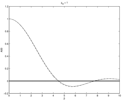
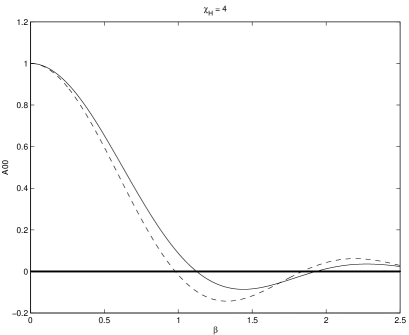
In Fig. 1 we give the transformed ‘top hat’ functions for two values of the horizon χHsubscript𝜒𝐻\chi_{H}, normalised to A00=1subscript𝐴001A_{00}=1 at β=0𝛽0\beta=0. When the horizon is less than or equal to the comoving curvature scale (χH1subscript𝜒𝐻1\chi_{H}\leq 1), we see that the open universe transform displays very similar behaviour to the flat space Bessel transform. However, on supercurvature scales (χH>1subscript𝜒𝐻1\chi_{H}>1), the open and flat universe transforms exhibit different behaviour. In particular, we shall choose the first zero of the ‘top hat’ transform as a means of describing the relationship between the horizon scale χHsubscript𝜒𝐻\chi_{H} and the corresponding value of the transformed variable βHsubscript𝛽𝐻\beta_{H} (the horizon mode wavenumber). From these we will calculate the value of

αβHχH,𝛼subscript𝛽𝐻subscript𝜒𝐻\alpha\equiv\beta_{H}\chi_{H}\,,

in order to discuss how this relationship is affected by curvature. The meaning of this relation is that, for a given χHsubscript𝜒𝐻\chi_{H}, those modes with βχH<α𝛽subscript𝜒𝐻𝛼\beta\chi_{H}<\alpha will have characteristic wavelengths larger than the horizon. Of course, for flat space and Cartesian coordinates, this relation is λ=2π/k<2π/kH=χH𝜆2𝜋𝑘2𝜋subscript𝑘𝐻subscript𝜒𝐻\lambda=2\pi/k<2\pi/k_{H}=\chi_{H}.

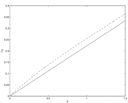
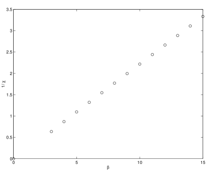
The first zeros of A00subscript𝐴00A_{00} in (24) are given by the solutions to

0=tanβχHβ×{tanhχH,K<0,χH,K=0,tanχH,K>0,0𝛽subscript𝜒𝐻𝛽casessubscript𝜒𝐻𝐾0subscript𝜒𝐻𝐾0subscript𝜒𝐻𝐾0\displaystyle 0=\tan\beta\chi_{H}-\beta\times\left\{\begin{array}[]{ll}\tanh\chi_{H}\;,&K<0\;,\\ \chi_{H}\;,&K=0\;,\\ \tan\chi_{H}\;,&K>0\;,\end{array}\right. (28)

which are shown in Fig. 2. Note from (24) that the zeros of (28) will be precisely the zeros of Φβ1subscriptsuperscriptΦ1𝛽\Phi^{1}_{\beta}, assuming χH>0subscript𝜒𝐻0\chi_{H}>0 (for K0𝐾0K\leq 0) and assuming 0<χH<π0subscript𝜒𝐻𝜋0<\chi_{H}<\pi for the closed (K>0𝐾0K>0) case.

The open and flat universes display phenomenologically similar curves. Certainly, as can be seen from Fig. 2, the curves are approximately parallel for χHsubscript𝜒𝐻\chi_{H} less than (or of the order of) the curvature scale, and that, on these scales, α𝛼\alpha is therefore the same (3π/2similar-toabsent3𝜋2\sim 3\pi/2) as for flat space: in the local limit, βχ=qykr𝛽𝜒𝑞𝑦𝑘𝑟\beta\chi=qy\longrightarrow kr when χ1much-less-than𝜒1\chi\ll 1 (y|K|much-less-than𝑦𝐾y\ll\sqrt{|K|}) or when |K|0𝐾0|K|\longrightarrow 0. However, for comoving distances much larger than χH4similar-tosubscript𝜒𝐻4\chi_{H}\sim 4 the effect of the curvature is to effectively shrink α𝛼\alpha as the curvature induced volume growth becomes significant. The corresponding limit is

αβHχHπasχH(K<0).formulae-sequence𝛼subscript𝛽𝐻subscript𝜒𝐻𝜋assubscript𝜒𝐻𝐾0\alpha\equiv\beta_{H}\chi_{H}\longrightarrow\pi\qquad\hbox{as}\qquad\chi_{H}\longrightarrow\infty\qquad(K<0)\,.

It is clear from this simple discussion that the characteristic lengthscale of a mode corresponding to the eigenvalue k𝑘k is given by 1/β1𝛽1/\beta.

Refer to caption
Refer to caption
FIG. 1.: The transformed ‘top hat’ function A00: K=0𝐾0K=0 (–), K=1𝐾1K=-1 (- -).

For an open universe, on very subhorizon or very superhorizon scales, we may simply take βτ1much-greater-than𝛽𝜏1\beta\tau\gg 1, or βτ1much-less-than𝛽𝜏1\beta\tau\ll 1 respectively, which is directly analogous to the flat space (k~τ1much-greater-than~𝑘𝜏1\tilde{k}\tau\gg 1, k~τ1much-less-than~𝑘𝜏1\tilde{k}\tau\ll 1) limits. However, we note that we must not neglect the precise location of the horizon if we are to describe the effect of the curvature scale upon the behaviour of the eigenfunctions. We shall return to this issue later (see §V), when we observe that curvature effects are significant from as early as τ=χH=0.5𝜏subscript𝜒𝐻0.5\tau=\chi_{H}=0.5.

At this point a brief comment on the difference between the Hubble radius and the particle horizon is relevant. In practice, causal perturbations are usually suppressed beyond the Hubble radius because this is roughly the maximum distance over which correlations can be established in one Hubble time. However, in principle, they can exist out to the particle horizon, so we must consider this distinction carefully (e.g. for cosmic strings or, in a more extreme case, for exploding neutrino shells). From the Friedmann equations (4) we see that the comoving Hubble radius 1=(1Ω)1/2<1superscript1superscript1Ω121{\cal H}^{-1}=(1-\Omega)^{1/2}<1 for an open universe, where the density parameter Ω=ρ/ρcritΩ𝜌subscript𝜌crit\Omega=\rho/\rho_{\rm crit} and ρcrit=32/κa2subscript𝜌crit3superscript2𝜅superscript𝑎2\rho_{\rm crit}=3{\cal H}^{2}/\kappa a^{2}. Clearly, this implies that the Hubble radius is always less than the curvature scale. In inflationary scenarios the Hubble radius is usually the most important quantity and this bound has been used to argue that perturbations with characteristic wavelengths smaller than the curvature scale are well modelled by a flat universe (see, for example, ref. [25]). However, the open universe particle horizon is obtained from the equation

sinh2(χH2)=1Ω1,superscript2subscript𝜒𝐻21Ω1\displaystyle\sinh^{2}\left(\frac{\chi_{H}}{2}\right)=\frac{1}{\Omega}-1\;, (29)

so that the proper distance dH=aχH2H1subscript𝑑𝐻𝑎subscript𝜒𝐻2superscript𝐻1d_{H}=a\chi_{H}\approx 2H^{-1} for Ω1Ω1\Omega\approx 1, where H1superscript𝐻1H^{-1} is the physical Hubble radius. It is therefore possible for the particle horizon to cross the curvature scale: χH>1subscript𝜒𝐻1\chi_{H}>1 for Ω<0.75Ω0.75\Omega<0.75. Moreover, in order for χH>0.5subscript𝜒𝐻0.5\chi_{H}>0.5 today (when curvature effects become more important — see §V) we require only that Ω<0.94Ω0.94\Omega<0.94 today. This is well within current observational constraints, and serves to motivate a more complete treatment of the physics around the curvature scale.
Refer to caption
Refer to caption
FIG. 2.: Solutions to (28): K=0𝐾0K=0 (–), K=1𝐾1K=-1 (- -), K=+1𝐾1K=+1 (o) .

For the closed (K>0𝐾0K>0) case we see that for the discrete spectrum β=3,4,𝛽34\beta=3,4,..., we have α3π/2𝛼3𝜋2\alpha\approx 3\pi/2, which goes over to the (continuous) flat space result in the limit χ0𝜒0\chi\rightarrow 0. We note that the notion of supercurvature and superhorizon perturbations with βαmuch-less-than𝛽𝛼\beta\ll\alpha, χH1much-greater-thansubscript𝜒𝐻1\chi_{H}\gg 1 does not have meaning in the closed universe. Indeed, from Fig. 2, we observe that all the β𝛽\beta have zeros for values of χHπ/2subscript𝜒𝐻𝜋2\chi_{H}\leq\pi/2, at which point the closed universe has its maximal circumference and surface area.

B The white noise spectrum

We may use causality and the superhorizon limit to establish that the correlators between pseudo-stress must go as a constant on superhorizon scales βχ𝐲αmuch-less-than𝛽subscript𝜒𝐲𝛼\beta\chi_{\bf y}\ll\alpha. Substituting the small argument series expansion of sinβχ𝛽𝜒\sin\beta\chi, in the exact expression (A13) for Φβ0(χ)subscriptsuperscriptΦ0𝛽𝜒\Phi^{0}_{\beta}(\chi), we find that the isotropic (l=0𝑙0l=0) mode for the correlator of two arbitrary scalar functions may be written as

f(𝐱)g(𝐱+𝐲)00(β)=n=0(1)nβ2n(2n+1)!dV𝐲<f(𝐱)g(𝐱+𝐲)>×{χ𝐲2n+1sinh(χ𝐲)K<0χ𝐲2nK=0χ𝐲2n+1sin(χ𝐲)K>0.subscriptdelimited-⟨⟩𝑓𝐱𝑔𝐱𝐲00𝛽subscriptsuperscript𝑛0superscript1𝑛superscript𝛽2𝑛2𝑛1differential-dsubscript𝑉𝐲expectation𝑓𝐱𝑔𝐱𝐲casessuperscriptsubscript𝜒𝐲2𝑛1sinhsubscript𝜒𝐲𝐾0superscriptsubscript𝜒𝐲2𝑛𝐾0superscriptsubscript𝜒𝐲2𝑛1sinsubscript𝜒𝐲𝐾0\displaystyle\langle f({\bf x})\;\;g({\bf x}+{\bf y})\rangle_{00}(\beta)=\sum^{\infty}_{n=0}\frac{(-1)^{n}\beta^{2n}}{(2n+1)!}\int{\rm d}V_{\bf y}\;\;<f({\bf x})\;\;g({\bf x}+{\bf y})>\times\left\{\begin{array}[]{ll}\frac{\chi_{\bf y}^{2n+1}}{{\rm sinh}(\chi_{\bf y})}&K<0\\ \chi_{\bf y}^{2n}&K=0\\ \frac{\chi_{\bf y}^{2n+1}}{{\rm sin}(\chi_{\bf y})}&K>0\end{array}\right.\;. (33)

On superhorizon scales, we have βα/χ𝐲much-less-than𝛽𝛼subscript𝜒𝐲\beta\ll\alpha/\chi_{\bf y} for a given comoving radius χ𝐲χHmuch-greater-thansubscript𝜒𝐲subscript𝜒𝐻\chi_{\bf y}\gg\chi_{H} (where the results of §IV A imply that π<α<3π/2𝜋𝛼3𝜋2\pi<\alpha<3\pi/2). On sufficiently superhorizon scales, we may therefore choose β1much-less-than𝛽1\beta\ll 1, and the lowest order contribution to (33) will be proportional to β0superscript𝛽0\beta^{0}. Hence, f(𝐱)g(𝐱+𝐲)00(β)β0proportional-tosubscriptdelimited-⟨⟩𝑓𝐱𝑔𝐱𝐲00𝛽superscript𝛽0\langle f({\bf x})\;\;g({\bf x}+{\bf y})\rangle_{00}(\beta)\propto\beta^{0}, provided that the integrals are finite, which will be the case if we appeal to causality to set <f(𝐱)g(𝐱+𝐲)>=0expectation𝑓𝐱𝑔𝐱𝐲0<f({\bf x})\;\;g({\bf x}+{\bf y})>=0 for large values of the radial variable χ𝐲subscript𝜒𝐲\chi_{\bf y}. This result confirms those by Avelino [9], Pen et al[3] and Veerarghavan and Stebbins [12] for K=0𝐾0K=0.

Moreover, as the vector and tensor eigenfunctions given in Appendix A are proportional to the scalar radial functions ΦβlsubscriptsuperscriptΦ𝑙𝛽\Phi^{l}_{\beta}, we can conclude that correlators of vectors and tensors will be premultiplied by a factor behaving as for the scalars. This is in agreement with the results of Durrer et al[5] for K=0𝐾0K=0, and corrects the common, but erroneous, conclusion that the flat space anisotropic stress power spectra go as k4superscript𝑘4k^{4} (see, for example, refs. [20, 29, 33]).

Note that, if we attempt to find the behaviour with respect to k𝑘k, we run into difficulties in describing the higher order corrections. This is a consequence of the fact that there will be a constant (curvature) contribution to the k0superscript𝑘0k^{0} term from each term β2nsuperscript𝛽2𝑛\beta^{2n} in the series expansion (33) of Φβ0(χ𝐲)subscriptsuperscriptΦ0𝛽subscript𝜒𝐲\Phi^{0}_{\beta}(\chi_{\bf y}).

V Superhorizon behaviour of the isotropic mode

Of the several arguments in the literature which use energy-momentum conservation to yield a k4superscript𝑘4k^{4} superhorizon power spectrum for flat universes, that provided by Avelino [9] is the most convincing — see also refs. [3, 11, 12]. Using Cartesian coordinates, and assuming that the volume is large enough to justify the ergodic hypothesis, we may equate spatial and ensemble averages, and Fourier transform the correlator of the stresses, arriving at

|τij(k,η)τkl(k,η)|=V1|𝐲|<dcd3yeı𝐤𝐲τij(𝐱,η)τkl(𝐱+𝐲,η).subscript𝜏𝑖𝑗𝑘𝜂superscriptsubscript𝜏𝑘𝑙𝑘superscript𝜂superscript𝑉1subscript𝐲subscript𝑑𝑐superscriptd3𝑦superscript𝑒italic-ı𝐤𝐲delimited-⟨⟩subscript𝜏𝑖𝑗𝐱𝜂subscript𝜏𝑘𝑙𝐱𝐲superscript𝜂\displaystyle|\tau_{ij}(k,\eta)\;\;\tau_{kl}^{*}(k,\eta^{\prime})|=V^{-1}\int_{|{\bf y}|<d_{c}}{\rm d}^{3}y\;\;e^{\imath{\bf k}\cdot{\bf y}}\langle\tau_{ij}({\bf x},\eta)\;\;\tau_{kl}({\bf x}+{\bf y},\eta^{\prime})\rangle\;. (34)

Here we have implicitly made use of the convolution theorem, and hence the property eı𝐤𝐲=eı𝐤𝐱eı𝐤(𝐱+𝐲)superscript𝑒italic-ı𝐤𝐲superscript𝑒italic-ı𝐤𝐱superscript𝑒italic-ı𝐤𝐱𝐲e^{\imath{\bf k}\cdot{\bf y}}=e^{-\imath{\bf k}\cdot{\bf x}}e^{\imath{\bf k}\cdot({\bf x+y})} of the exponential kernel used in Fourier theory, while causality implies that the correlator has compact support in 𝐲𝐲{\bf y}. Hence, on superhorizon scales (|𝐤|dc1much-less-than𝐤subscript𝑑𝑐1|{\bf k}|d_{c}\ll 1) we may neglect the exponential part of the integrand and find that the “power spectrum” of the pseudo–stresses 𝒫τij=V|τij|2/(2π)3subscript𝒫subscript𝜏𝑖𝑗𝑉superscriptsubscript𝜏𝑖𝑗2superscript2𝜋3{\cal P}_{\tau_{ij}}=V|\tau_{ij}|^{2}/(2\pi)^{3} approachs a constant: we have a white noise (k0superscript𝑘0k^{0}) spectrum. Noting that partial differentiation with respect to xisuperscript𝑥𝑖x^{i} is equivalent to multiplying the associated Fourier variable by kisubscript𝑘𝑖k_{i}, we may use energy-momentum conservation (36) to obtain the result:

𝒫τ00=V|τ00(k,η)|2(2π)3subscript𝒫subscript𝜏00𝑉superscriptsubscript𝜏00𝑘𝜂2superscript2𝜋3\displaystyle{\cal P}_{\tau_{00}}=V\frac{|\tau_{00}(k,\eta)|^{2}}{(2\pi)^{3}} =\displaystyle= kikjkkkl(2π)3ηiηdη1ηiη1dη2ηiηdη1ηiη1dη2×\displaystyle\frac{k_{i}k_{j}k_{k}k_{l}}{(2\pi)^{3}}\int_{\eta_{i}}^{\eta}{\rm d}\eta_{1}\int_{\eta_{i}}^{\eta_{1}}{\rm d}\eta_{2}\int_{\eta_{i}}^{\eta}{\rm d}\eta_{1}^{\prime}\int_{\eta_{i}}^{\eta_{1}^{\prime}}{\rm d}\eta_{2}^{\prime}\times (36)
|𝐲|<dcd3yτij(𝐱,η2)τkl(𝐱+𝐲,η2).subscript𝐲subscript𝑑𝑐superscriptd3𝑦delimited-⟨⟩subscript𝜏𝑖𝑗𝐱subscript𝜂2subscript𝜏𝑘𝑙𝐱𝐲superscriptsubscript𝜂2\displaystyle\int_{|{\bf y}|<d_{c}}{\rm d}^{3}y\;\;\langle\tau_{ij}({\bf x},\eta_{2})\;\;\tau_{kl}({\bf x}+{\bf y},\eta_{2}^{\prime})\rangle\;.

We conclude that, since τijτkldelimited-⟨⟩subscript𝜏𝑖𝑗subscript𝜏𝑘𝑙\langle\tau_{ij}\tau_{kl}\rangle exhibits white noise, then the power spectrum of τ00subscript𝜏00\tau_{00} should approach a k4superscript𝑘4k^{4} spectrum on superhorizon scales, as has been confirmed in numerical studies [34]. Similarly, the power spectrum of τi0subscriptsuperscript𝜏0𝑖\tau^{0}_{\;\;i} is proportional to k2superscript𝑘2k^{2}, in this limit.

The difficulty in generalising the above analysis to the general FRW universe lies in the lack of a useful equivalent to the exponential partial wave function in the general curved (K0𝐾0K\not=0) FRW universe (see ref. [27]), as well as in this argument’s dependence upon the choice of a Cartesian coordinate system. However, we can recast this argument using the eigenmodes of the Laplacian to investigate the constraints imposed by energy-momentum conservation and causality in both flat and instrinsically curved FRW universes, regaining also the familiar k4superscript𝑘4k^{4} spectrum in the local (or |K|0𝐾0|K|\longrightarrow 0) limit.

A Eigenmode splitting in curved spherical coordinates

In order to generalise this argument we must be able to split our eigenmodes in spherical coordinates under spatial translations to obtain an analogue of the convolution theorem. For the flat (K=0𝐾0K=0) FRW universe and spherical coordinates we have the relationship

j0(kr𝐲)=n=0(2n+1)jn(kr𝐱)jn(kr𝐱+𝐲)Pn(cosσ),subscript𝑗0𝑘subscript𝑟𝐲superscriptsubscript𝑛02𝑛1subscript𝑗𝑛𝑘subscript𝑟𝐱subscript𝑗𝑛𝑘subscript𝑟𝐱𝐲subscript𝑃𝑛𝜎\displaystyle j_{0}(kr_{\bf y})=\sum_{n=0}^{\infty}(2n+1)j_{n}(kr_{\bf x})j_{n}(kr_{{\bf x}+{\bf y}})P_{n}(\cos\sigma)\;, (37)

where σ𝜎\sigma is the angle between 𝐱𝐱-{\bf x} and 𝐱+𝐲𝐱𝐲{\bf x}+{\bf y} and we have used r𝐱=r𝐱subscript𝑟𝐱subscript𝑟𝐱r_{\bf-x}=r_{\bf x} [36]. In Appendix B we generalise this to the isotropic radial modes Φβ0(χ𝐲)subscriptsuperscriptΦ0𝛽subscript𝜒𝐲\Phi^{0}_{\beta}(\chi_{\bf y}) associated with general FRW spacetimes:

Φβ0(χ𝐲)=n=0(2n+1)Φβn(χ𝐱)Φβn(χ𝐱+𝐲)Pn(cosσ).subscriptsuperscriptΦ0𝛽subscript𝜒𝐲subscriptsuperscript𝑛02𝑛1subscriptsuperscriptΦ𝑛𝛽subscript𝜒𝐱subscriptsuperscriptΦ𝑛𝛽subscript𝜒𝐱𝐲subscript𝑃𝑛𝜎\displaystyle\Phi^{0}_{\beta}(\chi_{\bf y})=\sum^{\infty}_{n=0}(2n+1)\Phi^{n}_{\beta}(\chi_{\bf x})\Phi^{n}_{\beta}(\chi_{{\bf x}+{\bf y}})P_{n}(\cos\sigma)\;. (38)

The result (38) is valid for all 𝐲𝐲{\bf y}. We are, however, principally interested in the superhorizon limit, under which this relation simplifies greatly. In the superhorizon limit, it is easy to show that Φβl(χ)(βχ)lproportional-tosubscriptsuperscriptΦ𝑙𝛽𝜒superscript𝛽𝜒𝑙\Phi^{l}_{\beta}(\chi)\propto(\beta\chi)^{l}. Also, 𝐲𝐲{\bf y} superhorizon (βχ𝐲1much-less-than𝛽subscript𝜒𝐲1\beta\chi_{\bf y}\ll 1) implies that at least one of 𝐱𝐱-{\bf x}, 𝐱+𝐲𝐱𝐲{\bf x}+{\bf y} is superhorizon also, for any given 𝐱𝐱{\bf x}. Hence we can make use of the first order approximation only:

Φβ0(χ𝐲)Φβ0(χ𝐱)Φβ0(χ𝐱+𝐲),subscriptsuperscriptΦ0𝛽subscript𝜒𝐲subscriptsuperscriptΦ0𝛽subscript𝜒𝐱subscriptsuperscriptΦ0𝛽subscript𝜒𝐱𝐲\displaystyle\Phi^{0}_{\beta}(\chi_{\bf y})\approx\Phi^{0}_{\beta}(\chi_{\bf x})\Phi^{0}_{\beta}(\chi_{{\bf x}+{\bf y}})\;, (39)

for 𝐲𝐲{\bf y} superhorizon. Thus the lowest radial eigen-mode plays a role analogous to that of the exponential in Fourier theory.

While Appendix B provides a formal proof of the full expansion (38), here we just obtain (39). Consider an eigenfunction expansion of Φβ0(χ𝐮+𝐯)subscriptsuperscriptΦ0𝛽subscript𝜒𝐮𝐯\Phi^{0}_{\beta}(\chi_{\bf u+v}) in terms of Φβ0(χ𝐮)subscriptsuperscriptΦ0𝛽subscript𝜒𝐮\Phi^{0}_{\beta}(\chi_{\bf u}), after translation to 𝐮+𝐯𝐮𝐯{\bf u}+{\bf v}, which is given by

Φβ0(χ𝐮+𝐯)subscriptsuperscriptΦ0𝛽subscript𝜒𝐮𝐯\displaystyle\Phi^{0}_{\beta}(\chi_{{\bf u}+{\bf v}}) =\displaystyle= l,malmβ(𝐮)Φβl(χ𝐯)Ylm(θ𝐯,ϕ𝐯),subscript𝑙𝑚subscriptsuperscript𝑎𝛽𝑙𝑚𝐮subscriptsuperscriptΦ𝑙𝛽subscript𝜒𝐯subscript𝑌𝑙𝑚subscript𝜃𝐯subscriptitalic-ϕ𝐯\displaystyle\sum_{l,m}\;\;a^{\beta}_{lm}({\bf u})\Phi^{l}_{\beta}(\chi_{\bf v})Y_{lm}(\theta_{\bf v},\phi_{\bf v})\;, (40)
almβ(𝐮)subscriptsuperscript𝑎𝛽𝑙𝑚𝐮\displaystyle a^{\beta}_{lm}({\bf u}) =\displaystyle= 1NldV𝐯Φβ0(χ𝐮+𝐯)Φβl(χ𝐯)Ylm(θ𝐯,ϕ𝐯),1subscript𝑁𝑙differential-dsubscript𝑉𝐯subscriptsuperscriptΦ0𝛽subscript𝜒𝐮𝐯subscriptsuperscriptΦ𝑙𝛽subscript𝜒𝐯subscript𝑌𝑙𝑚subscript𝜃𝐯subscriptitalic-ϕ𝐯\displaystyle\frac{1}{N_{l}}\int{\rm d}V_{\bf v}\;\;\Phi^{0}_{\beta}(\chi_{{\bf u}+{\bf v}})\Phi^{l}_{\beta}(\chi_{\bf v})Y_{lm}(\theta_{\bf v},\phi_{\bf v})\;, (41)

where Nl=4πdV𝐯[Φβl(χ𝐯)Ylm(θ𝐯,ϕ𝐯)]2subscript𝑁𝑙4𝜋differential-dsubscript𝑉𝐯superscriptdelimited-[]subscriptsuperscriptΦ𝑙𝛽subscript𝜒𝐯subscript𝑌𝑙𝑚subscript𝜃𝐯subscriptitalic-ϕ𝐯2N_{l}=\sqrt{4\pi}\int{\rm d}V_{\bf v}\;\left[\Phi^{l}_{\beta}(\chi_{\bf v})Y_{lm}(\theta_{\bf v},\phi_{\bf v})\right]^{2}. We shall demonstrate that a00β(χ𝐮)=4πΦβ0(χ𝐮)subscriptsuperscript𝑎𝛽00subscript𝜒𝐮4𝜋subscriptsuperscriptΦ0𝛽subscript𝜒𝐮a^{\beta}_{00}(\chi_{\bf u})=\sqrt{4\pi}\Phi^{0}_{\beta}(\chi_{\bf u}), so that (for 𝐮=𝐱𝐮𝐱{\bf u}=-{\bf x} and 𝐯=𝐱+𝐲𝐯𝐱𝐲{\bf v}={\bf x}+{\bf y}) eqn (39) is confirmed, on superhorizon scales where this coefficient carries the leading order behaviour. Here, we give only the open universe argument, that for the K0𝐾0K\geq 0 cosmologies being similar. Substituting for the volume element, for the l=0𝑙0l=0 spherical harmonic, and for each of the two radial eigenfunctions using (A13), yields

a00β(χ𝐮+𝐯)=π|K|3/2β2N00dχ𝐯sinhχ𝐯sin(βχ𝐯)0πdθsinθsin(βχ𝐮+𝐯)sinhχ𝐮+𝐯.subscriptsuperscript𝑎𝛽00subscript𝜒𝐮𝐯𝜋superscript𝐾32superscript𝛽2subscript𝑁0subscriptsuperscript0differential-dsubscript𝜒𝐯sinhsubscript𝜒𝐯sin𝛽subscript𝜒𝐯subscriptsuperscript𝜋0differential-d𝜃sin𝜃sin𝛽subscript𝜒𝐮𝐯sinhsubscript𝜒𝐮𝐯\displaystyle a^{\beta}_{00}(\chi_{{\bf u}+{\bf v}})=\frac{\sqrt{\pi}}{|K|^{3/2}\beta^{2}N_{0}}\int^{\infty}_{0}{\rm d}\chi_{\bf v}\;\;{\rm sinh}\chi_{\bf v}{\rm sin}(\beta\chi_{\bf v})\int^{\pi}_{0}{\rm d}\theta\;\;{\rm sin}\theta\frac{{\rm sin}(\beta\chi_{{\bf u}+{\bf v}})}{{\rm sinh}\chi_{{\bf u}+{\bf v}}}\;. (42)

Changing variables from θ𝜃\theta to ξχ𝐮+𝐯𝜉subscript𝜒𝐮𝐯\xi\equiv\chi_{{\bf u}+{\bf v}} using (B2), we obtain the relation sinθdθ=sinhξdξ/sinhχ𝐯sinhχ𝐮sin𝜃d𝜃sinh𝜉d𝜉sinhsubscript𝜒𝐯sinhsubscript𝜒𝐮{\rm sin}\theta{\rm d}\theta={\rm sinh}\xi{\rm d}\xi/{\rm sinh}\chi_{\bf v}{\rm sinh}\chi_{{\bf u}}, and calculate the inner integral to be 2sin(βχ𝐯)sin(βχ𝐮+𝐯)βsinhχ𝐯sinhχ𝐮2sin𝛽subscript𝜒𝐯sin𝛽subscript𝜒𝐮𝐯𝛽sinhsubscript𝜒𝐯sinhsubscript𝜒𝐮\frac{2{\rm sin}(\beta\chi_{\bf v}){\rm sin}(\beta\chi_{{\bf u}+{\bf v}})}{\beta{\rm sinh}\chi_{\bf v}{\rm sinh}\chi_{\bf u}}. Hence,

a00β(χ𝐯)subscriptsuperscript𝑎𝛽00subscript𝜒𝐯\displaystyle a^{\beta}_{00}(\chi_{\bf v}) =\displaystyle= 2π|K|3/2β2N0sin(βχ𝐮)βsinhχ𝐮0dχ𝐯sin2βχ𝐯=4πsinβχ𝐮βsinhχ𝐮2𝜋superscript𝐾32superscript𝛽2subscript𝑁0sin𝛽subscript𝜒𝐮𝛽sinhsubscript𝜒𝐮subscriptsuperscript0differential-dsubscript𝜒𝐯superscriptsin2𝛽subscript𝜒𝐯4𝜋sin𝛽subscript𝜒𝐮𝛽sinhsubscript𝜒𝐮\displaystyle\frac{2\sqrt{\pi}}{|K|^{3/2}\beta^{2}N_{0}}\frac{{\rm sin}(\beta\chi_{{\bf u}})}{\beta{\rm sinh}\chi_{{\bf u}}}\int^{\infty}_{0}{\rm d}\chi_{\bf v}\;\;{\rm sin}^{2}\beta\chi_{\bf v}=\sqrt{4\pi}\frac{{\rm sin}\beta\chi_{{\bf u}}}{\beta{\rm sinh}\chi_{{\bf u}}} (43)
=\displaystyle= 4πΦβ0(χ𝐮),4𝜋subscriptsuperscriptΦ0𝛽subscript𝜒𝐮\displaystyle\sqrt{4\pi}\Phi^{0}_{\beta}(\chi_{{\bf u}})\;, (44)

where we have used the normalisation N0=(|K|3/2β2)10dχsin2βχsubscript𝑁0superscriptsuperscript𝐾32superscript𝛽21subscriptsuperscript0differential-d𝜒superscriptsin2𝛽𝜒N_{0}=({|K|^{3/2}\beta^{2}})^{-1}\int^{\infty}_{0}{\rm d}\chi\;{\rm sin}^{2}\beta\chi in the last equality. Observe that, formally, we should evaluate N0subscript𝑁0N_{0}, and effect the cancellation in (44), in terms of a limit of a volume larger than all length scales of interest.

B Integration by parts

Substituting (39) in (LABEL:00-dcor1), transforming the inner integration variable to 𝐱+𝐲𝐱𝐲{\bf x}+{\bf y}, and noting that the integrals are over all space so that dV𝐱+𝐲=dV𝐲dsubscript𝑉𝐱𝐲dsubscript𝑉𝐲{\rm d}V_{{\bf x}+{\bf y}}={\rm d}V_{\bf y}, we see that the l=0𝑙0l=0 mode is given by the double integral in 𝐱𝐱{\bf x} and 𝐱+𝐲𝐱𝐲{\bf x}+{\bf y}:

τj|ii|j(𝐱)τq|pp|q(𝐱+𝐲)00(k)\displaystyle\langle\tau^{i\;\;\;\;|j}_{\;\;j|i}({\bf x})\;\;\tau^{p\;\;\;\;|q}_{\;\;q|p}({\bf x}+{\bf y})\rangle_{00}(k) =\displaystyle= 12π2dV𝐱τj|ii|j(𝐱)Φβ0(χ𝐱)\displaystyle\frac{1}{\sqrt{2\pi^{2}}}\int{\rm d}V_{\bf x}\;\;\tau^{i\;\;\;\;|j}_{\;\;j|i}({\bf x})\Phi^{0}_{\beta}(\chi_{\bf x}) (46)
×dV𝐱+𝐲τj|ii|j(𝐱+𝐲)Φβ0(χ𝐱+𝐲).\displaystyle\times\int{\rm d}V_{{\bf x}+{\bf y}}\;\;\tau^{i\;\;\;\;|j}_{\;\;j|i}({\bf x}+{\bf y})\Phi^{0}_{\beta}(\chi_{{\bf x}+{\bf y}})\;.

In order to evaluate the integrals in (46) we make use of a generalised form of Gauss’s Law [35]

G3Wa;adV=G2WadSa,\displaystyle\int_{G^{3}}W_{a}^{\;\;;a}{\rm d}V=\int_{G^{2}}W_{a}{\rm dS^{a}}\;, (47)

where dV=g(3)dx1dx2dx3d𝑉superscript𝑔3dsuperscript𝑥1dsuperscript𝑥2dsuperscript𝑥3{\rm d}V=\sqrt{-g^{(3)}}\,{\rm d}x^{1}{\rm d}x^{2}{\rm d}x^{3} and dSa=g(3)abdSadsuperscript𝑆𝑎superscript𝑔3𝑎𝑏dsubscript𝑆𝑎{\rm d}S^{a}=g^{(3)ab}{\rm d}S_{a}, dSa=(1/2!)ϵam1m2d1xm1d2xm2dsubscript𝑆𝑎12subscriptitalic-ϵ𝑎subscript𝑚1subscript𝑚2subscriptd1superscript𝑥subscript𝑚1subscriptd2superscript𝑥subscript𝑚2{\rm d}S_{a}=(1/2!)\epsilon_{am_{1}m_{2}}{\rm d}_{1}x^{m_{1}}{\rm d}_{2}x^{m_{2}}. Here, we may choose the 333-dimensional vector components dixmisubscriptd𝑖superscript𝑥subscript𝑚𝑖{\rm d}_{i}x^{m_{i}} such that dxmidsuperscript𝑥subscript𝑚𝑖{\rm d}x^{m_{i}} appears as the i𝑖i-th component while the rest vanish (for instance, d2xm2=(0,dxm2,0)subscriptd2superscript𝑥subscript𝑚20dsuperscript𝑥subscript𝑚20{\rm d}_{2}x^{m_{2}}=(0,{\rm d}x^{m_{2}},0)). As we are on a constant time hypersurface, the index a𝑎a runs over 1,2,31231,2,3 only, as do the misubscript𝑚𝑖m_{i}.

Now, if we replace Wasuperscript𝑊𝑎W^{a} with fWa𝑓superscript𝑊𝑎fW^{a} in (47) where f𝑓f is some scalar quantity (so that f;a=f,af_{;a}=f_{,a}) and apply the chain rule, we obtain the result

G3dVfWa;a\displaystyle\int_{G^{3}}{\rm d}VfW_{a}^{\;\;;a} =\displaystyle= G3dV(fWa);aG3dVf,aWa\displaystyle\int_{G^{3}}{\rm d}V(fW_{a})^{;a}-\int_{G^{3}}{\rm d}Vf^{,a}W_{a} (48)
=\displaystyle= G2dSa(fWa)G3dVf,aWa.\displaystyle\int_{G^{2}}{\rm d}S^{a}(fW_{a})-\int_{G^{3}}{\rm d}Vf^{,a}W_{a}\;. (49)

This is the formal expression of spatial integration by parts on a constant time hypersurface, and a similar result holds with the covariant and contravariant indices interchanged. We shall exploit this result twice in each of the two integrals in (46).

We shall proceed in some detail for the integral over 𝐱𝐱{\bf x}. The 𝐱+𝐲𝐱𝐲{\bf x}+{\bf y} integral is similar. Since the τjisubscriptsuperscript𝜏𝑖𝑗\tau^{i}_{\;\;j} transform as tensors, setting f=Φβ0(χ𝐱)𝑓subscriptsuperscriptΦ0𝛽subscript𝜒𝐱f=\Phi^{0}_{\beta}(\chi_{\bf x}) and Wj=τj|iisubscript𝑊𝑗subscriptsuperscript𝜏𝑖conditional𝑗𝑖W_{j}=\tau^{i}_{\;\;j|i} so that fWj𝑓subscript𝑊𝑗fW_{j} is a vector, we find that

dV𝐱Φβ0(χ𝐱)τj|ii|j\displaystyle\int{\rm d}V_{\bf x}\;\;\Phi^{0}_{\beta}(\chi_{\bf x})\tau^{i\;\;\;\;|j}_{\;\;j|i} =\displaystyle= dV𝐱Φβ0(χ𝐱)Wj|j\displaystyle\int{\rm d}V_{\bf x}\Phi^{0}_{\beta}(\chi_{\bf x})W_{j}^{\;\;|j} (50)
=\displaystyle= dV𝐱[Φβ0(χ𝐱)Wj]|jdV𝐱[Φβ0(χ𝐱)],jWj\displaystyle\int{\rm d}V_{\bf x}\;\;\left[\Phi^{0}_{\beta}(\chi_{\bf x})W_{j}\right]^{|j}-\int{\rm d}V_{\bf x}\;\;\left[\Phi^{0}_{\beta}(\chi_{\bf x})\right]^{,j}W_{j} (51)
=\displaystyle= df𝐱j[Φβ0(χ𝐱)Wj]dV𝐱[Φβ0(χ𝐱)],jWj\displaystyle\int{\rm d}f_{\bf x}^{j}\;\;\left[\Phi^{0}_{\beta}(\chi_{\bf x})W_{j}\right]-\int{\rm d}V_{\bf x}\;\;\left[\Phi^{0}_{\beta}(\chi_{\bf x})\right]^{,j}W_{j} (52)
=\displaystyle= dV𝐱[Φβ0(χ𝐱)],jτj|ii,\displaystyle-\int{\rm d}V_{\bf x}\left[\Phi^{0}_{\beta}(\chi_{\bf x})\right]^{,j}\tau^{i}_{\;\;j|i}\;, (53)

where the third equality is obtained as in (49), and the fourth equality is obtained by substituting for Wjsubscript𝑊𝑗W_{j}, and assuming that the surface integral term vanishes. Explicitly, the surface integrals vanish for all but the angular integral over the radial surface at infinity, by symmetry, and periodicity. This remaining surface integral may be also be set to zero on physical grounds by using the conservation equations (7) to obtain

limRΦβ0(R)dΩ[τj|ii]R=limRΦβ0(R)dΩ[τ˙j0]R,subscript𝑅subscriptsuperscriptΦ0𝛽𝑅differential-dΩsubscriptdelimited-[]subscriptsuperscript𝜏𝑖conditional𝑗𝑖𝑅subscript𝑅subscriptsuperscriptΦ0𝛽𝑅differential-dΩsubscriptdelimited-[]subscriptsuperscript˙𝜏0𝑗𝑅\displaystyle\lim_{R\longrightarrow\infty}\Phi^{0}_{\beta}(R)\int{\rm d}\Omega\left[\tau^{i}_{\;\;j|i}\right]_{R}=\lim_{R\longrightarrow\infty}\Phi^{0}_{\beta}(R)\int{\rm d}\Omega\left[\dot{\tau}^{0}_{\;\;j}\right]_{R}\;, (54)

and by noting that beyond the horizon the functions [Φβ0τ˙j0]Rsubscriptdelimited-[]subscriptsuperscriptΦ0𝛽subscriptsuperscript˙𝜏0𝑗𝑅[\Phi^{0}_{\beta}\dot{\tau}^{0}_{\;\;j}]_{R} (although possibly non–zero) should not make a net contribution to the correlator. Physically, we may think of this as an expression of the fact that we do not expect there to be any net bulk momentum transfers across a radial surface on the very largest scales, since τ  0jsubscriptsuperscript𝜏𝑗  0\tau^{j}_{\;\;0} is proportional to a well-defined momentum [17]. This is a much less stringent requirement than that previously imposed (i.e. that the functions themselves go to zero beyond the horizon [3, 19]) which is not expected to be true in most physical situations of interest. Our physically motivated and much weaker assumption thus allows for a more complete analysis of the superhorizon behaviour.

Repeating the analysis, we find that

dV𝐱Φβ0(χ𝐱)τj|ii|j=+dV𝐱{[Φβ0(χ𝐱)],j}|iτji,\displaystyle\int{\rm d}V_{\bf x}\;\;\Phi^{0}_{\beta}(\chi_{\bf x})\tau^{i\;\;\;\;|j}_{\;\;j|i}=+\int{\rm d}V_{\bf x}\;\;\left\{\left[\Phi^{0}_{\beta}(\chi_{\bf x})\right]^{,j}\right\}_{|i}\tau^{i}_{\;\;j}\;, (55)

where we have once again ignored the surface terms. Explicitly, the only non-trivial surface term is again the radial surface at infinity:

limRΦβ0(R)RdΩ𝐱[τ  1i]Rsubscript𝑅subscriptsuperscriptΦ0𝛽𝑅𝑅differential-dsubscriptΩ𝐱subscriptdelimited-[]subscriptsuperscript𝜏𝑖1𝑅\displaystyle\lim_{R\longrightarrow\infty}\frac{\partial\Phi^{0}_{\beta}(R)}{\partial R}\int{\rm d}\Omega_{\bf x}\left[\tau^{i}_{\;\;1}\right]_{R} (56)

and, this time, we expect there to be no net anisotropic shears across the radial surface on the largest scales, so that this surface term averages to zero and may be ignored. Hence, using the connection coefficients, as well as the derivative (A25) and recursion (A21) relations for the Φl0subscriptsuperscriptΦ0𝑙\Phi^{0}_{l}, we see that

dV𝐱Φβ0(χ𝐱)τj|ii|j=dV𝐱Φβ0fK(τ  22+τ  33)+dV𝐱Φβ0(χ)[k~2+2fK]τ  11,\displaystyle\int{\rm d}V_{\bf x}\;\;\Phi^{0}_{\beta}(\chi_{\bf x})\tau^{i\;\;\;\;|j}_{\;\;j|i}=-\int{\rm d}V_{\bf x}\;\;\Phi^{0}_{\beta}f_{K}\left(\tau^{2}_{\;\;2}+\tau^{3}_{\;\;3}\right)+\int{\rm d}V_{\bf x}\;\;\Phi^{0}_{\beta}(\chi)\left[-\tilde{k}^{2}+2f_{K}\right]\tau^{1}_{\;\;1}\;, (57)

where

fK(β,χ)cotK2χβcotKcot(βχ),subscript𝑓𝐾𝛽𝜒subscriptsuperscript2𝐾𝜒𝛽subscript𝐾𝛽𝜒\displaystyle f_{K}(\beta,\chi)\equiv\cot^{2}_{K}\chi-\beta\cot_{K}\cot(\beta\chi)\;, (58)

and cotKχ=cosKχ/sinKχsubscript𝐾𝜒subscript𝐾𝜒subscript𝐾𝜒\cot_{K}\chi=\cos_{K}\chi/\sin_{K}\chi where cosKχ={coshχ,χ,cosχ}subscript𝐾𝜒𝜒𝜒𝜒\cos_{K}\chi=\left\{\cosh\chi,\chi,\cos\chi\right\} for {K<0,\left\{K<0,\right. K=0,𝐾0K=0, K>0}\left.K>0\right\}.

Proceeding in a similar fashion for the 𝐱+𝐲𝐱𝐲{\bf x}+{\bf y} integral, multiplying to obtain four double integrals, and then reversing the steps that led to (46) — i.e. transforming back to 𝐲𝐲{\bf y} as the integration variable in the inner integral, and appealing to (39) — we may write the 000000–mode as

τj|ii|jτq|pp|q00(β)=\displaystyle\langle\tau^{i\;\;\;\;|j}_{\;\;j|i}\;\;\tau^{p\;\;\;\;|q}_{\;\;q|p}\rangle_{00}(\beta)= (59)
[k~2+2fK(β,χ𝐱)]τ  11(𝐱)[k~2+2fK(β,χ𝐱+𝐲)]τ  11(𝐱+𝐲)00(β)subscriptdelimited-⟨⟩delimited-[]superscript~𝑘22subscript𝑓𝐾𝛽subscript𝜒𝐱subscriptsuperscript𝜏11𝐱delimited-[]superscript~𝑘22subscript𝑓𝐾𝛽subscript𝜒𝐱𝐲subscriptsuperscript𝜏11𝐱𝐲00𝛽\displaystyle\;\;\;\;\;\langle\left[-\tilde{k}^{2}+2f_{K}(\beta,\chi_{\bf x})\right]\tau^{1}_{\;\;1}({\bf x})\;\;\left[-\tilde{k}^{2}+2f_{K}(\beta,\chi_{\bf x+y})\right]\tau^{1}_{\;\;1}({\bf x}+{\bf y})\rangle_{00}(\beta) (60)
+[k~2+2fK(β,χ𝐱)]τ  11(𝐱)[fK(β,χ𝐱+𝐲)](τ  22+τ  33)(𝐱+𝐲)00(β)subscriptdelimited-⟨⟩delimited-[]superscript~𝑘22subscript𝑓𝐾𝛽subscript𝜒𝐱subscriptsuperscript𝜏11𝐱delimited-[]subscript𝑓𝐾𝛽subscript𝜒𝐱𝐲subscriptsuperscript𝜏22subscriptsuperscript𝜏33𝐱𝐲00𝛽\displaystyle\;\;\;\;\;+\langle\left[-\tilde{k}^{2}+2f_{K}(\beta,\chi_{\bf x})\right]\tau^{1}_{\;\;1}({\bf x})\;\;\left[-f_{K}(\beta,\chi_{\bf x+y})\right]\left(\tau^{2}_{\;\;2}+\tau^{3}_{\;\;3}\right)({\bf x}+{\bf y})\rangle_{00}(\beta) (61)
+fK(β,χ𝐱)(τ  22+τ  33)(𝐱)[k~2+2fK(β,χ𝐱+𝐲)]τ  11(𝐱+𝐲)00(β)subscriptdelimited-⟨⟩subscript𝑓𝐾𝛽subscript𝜒𝐱subscriptsuperscript𝜏22subscriptsuperscript𝜏33𝐱delimited-[]superscript~𝑘22subscript𝑓𝐾𝛽subscript𝜒𝐱𝐲subscriptsuperscript𝜏11𝐱𝐲00𝛽\displaystyle\;\;\;\;\;+\langle-f_{K}(\beta,\chi_{\bf x})\left(\tau^{2}_{\;\;2}+\tau^{3}_{\;\;3}\right)({\bf x})\;\;\left[-\tilde{k}^{2}+2f_{K}(\beta,\chi_{\bf x+y})\right]\tau^{1}_{\;\;1}({\bf x}+{\bf y})\rangle_{00}(\beta) (62)
+fK(β,χ𝐱)(τ  22+τ  33)(𝐱)[fK(β,χ𝐱+𝐲)](τ  22+τ  33)(𝐱+𝐲)00(β).subscriptdelimited-⟨⟩subscript𝑓𝐾𝛽subscript𝜒𝐱subscriptsuperscript𝜏22subscriptsuperscript𝜏33𝐱delimited-[]subscript𝑓𝐾𝛽subscript𝜒𝐱𝐲subscriptsuperscript𝜏22subscriptsuperscript𝜏33𝐱𝐲00𝛽\displaystyle\;\;\;\;\;+\langle-f_{K}(\beta,\chi_{\bf x})\left(\tau^{2}_{\;\;2}+\tau^{3}_{\;\;3}\right)({\bf x})\;\;\left[-f_{K}(\beta,\chi_{\bf x+y})\right]\left(\tau^{2}_{\;\;2}\;\;\;+\tau^{3}_{\;\;3}\right)({\bf x}+{\bf y})\rangle_{00}(\beta)\;. (63)
(64)

Each of the four correlators on the right hand side of (64) is equal to a double integral similar in form (though, clearly not in integrand) to (46). As remarked earlier, for 𝐲𝐲{\bf y} superhorizon, at least one of 𝐱𝐱{\bf x}, 𝐱+𝐲𝐱𝐲{\bf x+y} is superhorizon also so that we may take the integral over that variable to be finite. Effectively, then, we have obtained the transfromed two-point correlators of the contracted derivatives of the pseudo-stresses—and hence the pseudo-energy—in terms of functions of k𝑘k times the transformed pseudo-stresses.

C Flat space

For the flat space (K=0𝐾0K=0) case, on sufficiently superhorizon scales (kr1much-less-than𝑘𝑟1kr\ll 1) we may take the limit

fK=0=1r2kcot(kr)rk23forkr1,formulae-sequencesubscript𝑓𝐾01superscript𝑟2𝑘cot𝑘𝑟𝑟superscript𝑘23much-less-thanfor𝑘𝑟1\displaystyle f_{K=0}=\frac{1}{r^{2}}-\frac{k{\rm cot}(kr)}{r}\approx\frac{k^{2}}{3}\hskip 14.22636pt{\rm for}\hskip 8.53581ptkr\ll 1\;, (65)

to show that the pre-factors (k2+2fK=0)2superscriptsuperscript𝑘22subscript𝑓𝐾02(-k^{2}+2f_{K=0})^{2}, fK=0(k2+2fK=0)subscript𝑓𝐾0superscript𝑘22subscript𝑓𝐾0-f_{K=0}(-k^{2}+2f_{K=0}), fK=02superscriptsubscript𝑓𝐾02f_{K=0}^{2} are functions of k𝑘k only, in the limit kr0𝑘𝑟0kr\longrightarrow 0. Hence, we may pull these factors out of the (implicit) integrals in (64) and, taking the limit to infinity, we obtain

τj|ii|jτq|pp|q00(k)\displaystyle\langle\tau^{i\;\;\;\;|j}_{\;\;j|i}\;\;\tau^{p\;\;\;\;|q}_{\;\;q|p}\rangle_{00}(k) =\displaystyle= k49[τ  11τ  1100(k)+τ  11(τ  22+τ  33)00(k)\displaystyle\frac{k^{4}}{9}\left[\langle\tau^{1}_{\;\;1}\;\;\tau^{1}_{\;\;1}\rangle_{00}(k)+\langle\tau^{1}_{\;\;1}\;\left(\tau^{2}_{\;\;2}+\tau^{3}_{\;\;3}\right)\rangle_{00}(k)\right. (67)
+(τ  22+τ  33)τ  1100(k)+(τ  22+τ  33)(τ  22+τ  33)00(k)],\displaystyle\left.+\langle\left(\tau^{2}_{\;\;2}+\tau^{3}_{\;\;3}\right)\;\tau^{1}_{\;\;1}\rangle_{00}(k)+\langle\left(\tau^{2}_{\;\;2}+\tau^{3}_{\;\;3}\right)\;\left(\tau^{2}_{\;\;2}+\tau^{3}_{\;\;3}\right)\rangle_{00}(k)\right]\;,

where the correlators on the right hand side of (LABEL:int-6) are known (see §IV B) to be proportional to k0superscript𝑘0k^{0} in this limit. Hence, appealing to the conservation equations (7) and noting that time differentiation does not affect β𝛽\beta-dependence in our eigenfunction expansions, we regain the familiar k4superscript𝑘4k^{4} power spectrum, as the spectrum for the 000000-mode

τ  00(𝐱)τ  00(𝐱+𝐲)00(k)k4.proportional-tosubscriptdelimited-⟨⟩subscriptsuperscript𝜏0  0𝐱subscriptsuperscript𝜏0  0𝐱𝐲00𝑘superscript𝑘4\displaystyle\langle\tau^{0}_{\;\;0}({\bf x})\;\;\tau^{0}_{\;\;0}({\bf x}+{\bf y})\rangle_{00}(k)\propto k^{4}\;. (69)

D Open universe

In this case, there are three regimes of interest: supercurvature, sub–curvature, and the case in which χ𝜒\chi is near the curvature scale. On superhorizon, supercurvature scales, χ1much-greater-than𝜒1\chi\gg 1, βχ1much-less-than𝛽𝜒1\beta\chi\ll 1 which implies that β1/χ1much-less-than𝛽1𝜒much-less-than1\beta\ll 1/\chi\ll 1. Hence, we have that cothχ1hyperbolic-cotangent𝜒1{\rm\coth}\chi\approx 1 and k~1~𝑘1\tilde{k}\approx 1, where these approximations are exact in this limit, and about which we have the expansion

fK<0(β,χ)=1βcot(βχ)=11χ+β2χ3=O(1),βχ1,χ1.formulae-sequencesubscript𝑓𝐾0𝛽𝜒1𝛽𝛽𝜒11𝜒superscript𝛽2𝜒3𝑂1formulae-sequencemuch-less-than𝛽𝜒1much-greater-than𝜒1\displaystyle f_{K<0}(\beta,\chi)=1-\beta\cot(\beta\chi)=1-\frac{1}{\chi}+\frac{\beta^{2}\chi}{3}\cdot\cdot\cdot=O(1)\;,\hskip 28.45274pt\beta\chi\ll 1\;,\;\;\chi\gg 1\;. (70)
(71)

Substituting (71) into (64), we see that the 000000-mode tends to a constant on supercurvature, and superhorizon scales. Explicitly, making the k~1~𝑘1\tilde{k}\approx 1 approximation valid on these superhorizon and supercurvature scales, we obtain

τj|ii|jτj|ii|j00(β)\displaystyle\langle\tau^{i\;\;\;\;|j}_{\;\;j|i}\;\;\tau^{i\;\;\;\;|j}_{\;\;j|i}\rangle_{00}(\beta) =\displaystyle= a1τ  11τ  1100(β)+a2τ  11(τ  22+τ  33)00(β)subscript𝑎1subscriptdelimited-⟨⟩subscriptsuperscript𝜏11subscriptsuperscript𝜏1100𝛽subscript𝑎2subscriptdelimited-⟨⟩subscriptsuperscript𝜏11subscriptsuperscript𝜏22subscriptsuperscript𝜏3300𝛽\displaystyle a_{1}\langle\tau^{1}_{\;\;1}\;\;\tau^{1}_{\;\;1}\rangle_{00}(\beta)+a_{2}\langle\tau^{1}_{\;\;1}\;\left(\tau^{2}_{\;\;2}+\tau^{3}_{\;\;3}\right)\rangle_{00}(\beta) (73)
+a3(τ  22+τ  33)τ  1100(β)+a4(τ  22+τ  33)(τ  22+τ  33)00(β),subscript𝑎3subscriptdelimited-⟨⟩subscriptsuperscript𝜏22subscriptsuperscript𝜏33subscriptsuperscript𝜏1100𝛽subscript𝑎4subscriptdelimited-⟨⟩subscriptsuperscript𝜏22subscriptsuperscript𝜏33subscriptsuperscript𝜏22subscriptsuperscript𝜏3300𝛽\displaystyle+a_{3}\langle\left(\tau^{2}_{\;\;2}+\tau^{3}_{\;\;3}\right)\;\tau^{1}_{\;\;1}\rangle_{00}(\beta)+a_{4}\langle\left(\tau^{2}_{\;\;2}+\tau^{3}_{\;\;3}\right)\;\left(\tau^{2}_{\;\;2}+\tau^{3}_{\;\;3}\right)\rangle_{00}(\beta)\;,
forfor\displaystyle\hskip 85.35826pt{\rm for} χ𝐱,𝐲1,βχ𝐱,𝐲1,formulae-sequencemuch-greater-thansubscript𝜒𝐱𝐲1much-less-than𝛽subscript𝜒𝐱𝐲1\displaystyle\hskip 28.45274pt\chi_{{\bf x},{\bf y}}\gg 1,\hskip 14.22636pt\beta\chi_{{\bf x},{\bf y}}\ll 1\;, (74)

where the aisubscript𝑎𝑖a_{i} are constant factors. Recalling the equations of motion (7) for the energy-momentum pseudo-tensor, and that the correlator between two arbitrary functions goes as β0superscript𝛽0\beta^{0}, we see that on very supercurvature and very superhorizon scales, the correlators behave as:

τ  00τ  0000β0.proportional-tosubscriptdelimited-⟨⟩subscriptsuperscript𝜏0  0subscriptsuperscript𝜏0  000superscript𝛽0\displaystyle\langle\tau^{0}_{\;\;0}\;\;\tau^{0}_{\;\;0}\rangle_{00}\;\;\propto\;\;\beta^{0}\;. (75)

Turning now to the other asymptote, we consider the case in which the horizon is very much less than the curvature scale. Then, on superhorizon, and very much subcurvature scales, we regain the familiar k4superscript𝑘4k^{4} power spectrum, up to a constant factor. Using the series expansions appropriate for χ1much-less-than𝜒1\chi\ll 1 and βχ1much-less-than𝛽𝜒1\beta\chi\ll 1, one easily finds that

fK<0=β2+13=k~23,βχ1,χ1.formulae-sequencesubscript𝑓𝐾0superscript𝛽213superscript~𝑘23formulae-sequencemuch-less-than𝛽𝜒1much-less-than𝜒1\displaystyle f_{K<0}=\frac{\beta^{2}+1}{3}=\frac{\tilde{k}^{2}}{3}\;,\hskip 28.45274pt\beta\chi\ll 1\;,\chi\ll 1\;. (76)

This has the same form as the superhorizon limit of fK=0subscript𝑓𝐾0f_{K=0}. However, one should recall that, while β𝛽\beta (for the K<0𝐾0K<0 case) and k𝑘k (for K=0𝐾0K=0) have similar spectra, their meanings are different in the two spacetimes — see equation (12). In particular, we have, for the open universe with χ1much-less-than𝜒1\chi\ll 1, two cases: β<1𝛽1\beta<1 and β>1𝛽1\beta>1. These correspond to mode wavelengths approximately equal to and smaller than the curvature horizon, respectively. In the former case, fK<01/3subscript𝑓𝐾013f_{K<0}\approx 1/3 and k~1~𝑘1\tilde{k}\approx 1 so that we have the result (75) once more. In the latter, fK<0β2/3subscript𝑓𝐾0superscript𝛽23f_{K<0}\approx\beta^{2}/3, for large β𝛽\beta, in which case we also have that k~2β2superscript~𝑘2superscript𝛽2\tilde{k}^{2}\approx\beta^{2}. Then, recalling the normalisation of k𝑘k, we have the local (subcurvature) superhorizon limit:

fK<0(χ,β)1|K|fK=0(k~,r).subscript𝑓𝐾0𝜒𝛽1𝐾subscript𝑓𝐾0~𝑘𝑟\displaystyle f_{K<0}(\chi,\beta)\approx\frac{1}{|K|}f_{K=0}(\tilde{k},r)\;. (77)

Recalling the conservation equations (7), this means that

τ  00(𝐱)τ  00(𝐱+𝐲)00(β)k~4=k4|K|2β4,χ𝐱,𝐲1,βχ𝐱,𝐲1,formulae-sequenceproportional-tosubscriptdelimited-⟨⟩subscriptsuperscript𝜏0  0𝐱subscriptsuperscript𝜏0  0𝐱𝐲00𝛽superscript~𝑘4superscript𝑘4superscript𝐾2superscript𝛽4formulae-sequencemuch-less-thansubscript𝜒𝐱𝐲1much-less-than𝛽subscript𝜒𝐱𝐲1\displaystyle\langle\tau^{0}_{\;\;0}({\bf x})\;\;\tau^{0}_{\;\;0}({\bf x}+{\bf y})\rangle_{00}(\beta)~{}\propto~{}\tilde{k}^{4}=\frac{k^{4}}{|K|^{2}}\approx\beta^{4},\hskip 22.76219pt\chi_{{\bf x},{\bf y}}\ll 1,\hskip 14.22636pt\beta\chi_{{\bf x},{\bf y}}\ll 1\;, (78)

where k𝑘k is the flat space Fourier wavenumber.

Having dealt with both the extreme cases of local flatness and curvature domination, there remains the interesting question of the behaviour near the curvature scale. We therefore would like to understand how the k4superscript𝑘4k^{4} superhorizon behaviour on sub–curvature scales becomes β0=k0superscript𝛽0superscript𝑘0\beta^{0}=k^{0} on very super–curvature scales, and the ranges within which these approximations are valid.

Away from the asymptotes dealt with above, fK<0subscript𝑓𝐾0f_{K<0} is a function of the radial coordinate, and therefore is integrated over (twice) in equation (64). This means that we may only truly understand the effect of the factors in this equation by explicitly calculating the integral, which requires that we specify the pseudo–stresses. As a first approximation, however, we may proceed to obtain some understanding of the superhorizon behaviour of generic causal perturbations by assuming that the corrections are small enough for us to make the approximation

<τ  00(𝐱)τ  00(𝐱+𝐲)>00(P1+P2+P3+P4)A00,subscriptexpectationsubscriptsuperscript𝜏0  0𝐱subscriptsuperscript𝜏0  0𝐱𝐲00𝑃1𝑃2𝑃3𝑃4subscript𝐴00\displaystyle<\tau^{0}_{\;\;0}({\bf x})\;\;\tau^{0}_{\;\;0}({\bf x+y})>_{00}~{}\approx~{}(P1+P2+P3+P4)A_{00}\;, (79)

where

P1=(k~2+2fK<0)2,P2=fK<0(k~2+2fK<0),P3=(k~2+2fK<0)fK<0,P4=fK<02,𝑃1superscriptsuperscript~𝑘22subscript𝑓𝐾02𝑃2subscript𝑓𝐾0superscript~𝑘22subscript𝑓𝐾0𝑃3superscript~𝑘22subscript𝑓𝐾0subscript𝑓𝐾0𝑃4superscriptsubscript𝑓𝐾02\displaystyle\begin{array}[]{ll}P1=(-\tilde{k}^{2}+2f_{K<0})^{2}\;,&P2=-f_{K<0}(-\tilde{k}^{2}+2f_{K<0})\;,\\ P3=-(-\tilde{k}^{2}+2f_{K<0})f_{K<0}\;,&P4=f_{K<0}^{2}\;,\end{array} (82)

for some given χ𝜒\chi, and where we have assumed that the correlators of the τjisubscriptsuperscript𝜏𝑖𝑗\tau^{i}_{\;\;j} are well modelled by window functions of the form used in §IV A. This assumption amounts to ignoring long range correlations, since we assume that χ𝐱χ𝐱+𝐲subscript𝜒𝐱subscript𝜒𝐱𝐲\chi_{\bf x}\approx\chi_{\bf x+y}. Hence this approximation is valid for χ𝐲subscript𝜒𝐲\chi_{\bf y} small, that is, in the very early universe.

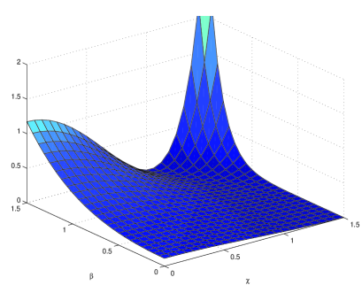
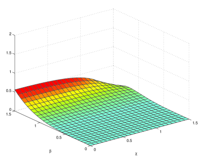
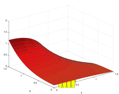
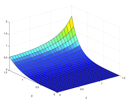
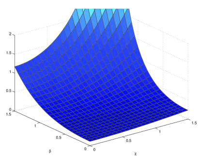
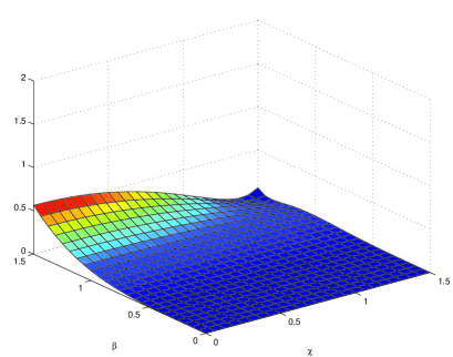
We provide surface plots for these pre-factors in Figures 35, from which we can clearly see how our approximations are valid only for χ<0.5𝜒0.5\chi<0.5, and break down as we move into the large χ𝜒\chi and large β𝛽\beta regime, doing so much earlier than in the K=0𝐾0K=0 scenario. This is a geometric effect due to the fact that the majority of the volume in a hyperbolic space is located near the radial surface, so that a large ‘hyper-sphere’ approximates a ‘hyper-shell’. This effect is most noticible on supercurvature scales. However, one can calculate that the ratio of hyperbolic volume to surface area rapidly diverges from that for a spherical geometry, beginning at around χ0.5similar-to𝜒0.5\chi\sim 0.5. On the other hand, the steep slope in the prefactor P1subscript𝑃1P_{1} for large β𝛽\beta and χ<0.4𝜒0.4\chi<0.4 is due to the appearance of a constant (curvature) term in the (repeated) k~~𝑘\tilde{k} factors in this prefactor. However, as χ𝜒\chi increases, so does fK<0subscript𝑓𝐾0f_{K<0}, first cancelling, and then overriding this effect. Along the β𝛽\beta axis in each plot (i.e. for χ0similar-to𝜒0\chi\sim 0), we see that all the pre-factors go as k4/9superscript𝑘49k^{4}/9 for K=0𝐾0K=0 and as (β2+1)2/9superscriptsuperscript𝛽2129(\beta^{2}+1)^{2}/9 for K=1𝐾1K=-1. Along the χ𝜒\chi axis (β0similar-to𝛽0\beta\sim 0), all the pre-factors vanish for K=0𝐾0K=0. However, for the K=1𝐾1K=-1 case, this is not the case, reflecting the small constant (curvature) term.
Refer to caption
Refer to caption
FIG. 3.: P1: K = 0 (LHS), and K = -1 (RHS)
Refer to caption
Refer to caption
FIG. 4.: P2 = P3 (in this limit): K = 0 (LHS), K = -1 (RHS)
Refer to caption
Refer to caption
FIG. 5.: P4: K = 0 (LHS), K = -1 (RHS)
Refer to caption
Refer to caption
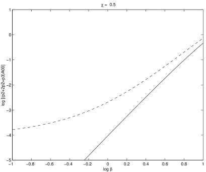
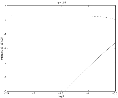
FIG. 6.: Log (P1 + 2P2 + P3)A00 for K = 0 (-) and K = -1 (- - -)

Computing τ  00τ  00delimited-⟨⟩subscriptsuperscript𝜏0  0subscriptsuperscript𝜏0  0\langle\tau^{0}_{\;\;0}\;\;\tau^{0}_{\;\;0}\rangle using the approximation (79) we find the curves plotted in Figure 6. These show clearly how the k4superscript𝑘4k^{4} behaviour on superhorizon scales is flattened out, for small β𝛽\beta, by the intrinsic curvature. We note that this does not mean that we expect the real space correlators to similarly go to a constant on these scales because, of course, they vanish by causality. Integrating (79) over all β𝛽\beta, with the kernel Φβ0subscriptsuperscriptΦ0𝛽\Phi^{0}_{\beta}, the constant term is suppressed by the measure dμ(β)=β2dβd𝜇𝛽superscript𝛽2d𝛽{\rm d}\mu(\beta)=\beta^{2}{\rm d}\beta. Similarly, calculating the variance

σ2=0dμ(β)τ  00τ  0000(β)=01dμ(β)τ  00τ  0000(β)+1dμ(β)τ  00τ  0000(β),superscript𝜎2superscriptsubscript0differential-d𝜇𝛽subscriptdelimited-⟨⟩subscriptsuperscript𝜏0  0subscriptsuperscript𝜏0  000𝛽superscriptsubscript01differential-d𝜇𝛽subscriptdelimited-⟨⟩subscriptsuperscript𝜏0  0subscriptsuperscript𝜏0  000𝛽superscriptsubscript1differential-d𝜇𝛽subscriptdelimited-⟨⟩subscriptsuperscript𝜏0  0subscriptsuperscript𝜏0  000𝛽\displaystyle\sigma^{2}=\int_{0}^{\infty}{\rm d}\mu(\beta)\langle\tau^{0}_{\;\;0}\;\;\tau^{0}_{\;\;0}\rangle_{00}(\beta)=\int_{0}^{1}{\rm d}\mu(\beta)\langle\tau^{0}_{\;\;0}\;\;\tau^{0}_{\;\;0}\rangle_{00}(\beta)+\int_{1}^{\infty}{\rm d}\mu(\beta)\langle\tau^{0}_{\;\;0}\;\;\tau^{0}_{\;\;0}\rangle_{00}(\beta)\;, (83)

and breaking the integral over all β𝛽\beta into supercurvature and subcurvature parts, we see that the second integral is procedurally the same as for the flat space case, for both sub- and superhorizon scales, while the first (containing the constant power spectrum constribution) is suppressed by the β2superscript𝛽2\beta^{2} factor in the measure.

E Closed universe

For the closed universe we have the prefactors determined by

fK>0(β,χ)=cot2χβcotχcot(βχ).subscript𝑓𝐾0𝛽𝜒superscriptcot2𝜒𝛽𝜒𝛽𝜒\displaystyle f_{K>0}(\beta,\chi)={\rm cot}^{2}\chi-\beta\cot\chi\cot(\beta\chi)\;. (84)

The difference between the open and closed universe cases is quantified by the differences between the behaviour of the function (84) and that of fK<0subscript𝑓𝐾0f_{K<0}. To begin with, the eigenspectrum for β𝛽\beta is discrete, and the lowest non-gauge mode is β=3𝛽3\beta=3 so that the superhorizon limit βχH1much-less-than𝛽subscript𝜒𝐻1\beta\chi_{H}\ll 1 can only be attained for χH1/3much-less-thansubscript𝜒𝐻13\chi_{H}\ll 1/3. Of course, for χH1much-greater-thansubscript𝜒𝐻1\chi_{H}\gg 1 we encounter the periodic properties the closed universe: one cannot have modes that are both superhorizon and supercurvature.

If we take χ1much-less-than𝜒1\chi\ll 1 and βχ1much-less-than𝛽𝜒1\beta\chi\ll 1, then we consider the subcurvature yet superhorizon case. Here, we note that cotχ1/χχ/3𝜒1𝜒𝜒3\cot\chi\approx 1/\chi-\chi/3, wo we have

fK>0=β213=k~23,βχ1,χ1,formulae-sequencesubscript𝑓𝐾0superscript𝛽213superscript~𝑘23formulae-sequencemuch-less-than𝛽𝜒1much-less-than𝜒1\displaystyle f_{K>0}=\frac{\beta^{2}-1}{3}=\frac{\tilde{k}^{2}}{3}\;,\hskip 28.45274pt\beta\chi\ll 1,\;\;\;\chi\ll 1\;, (85)

and we regain the flat space results in a similar fashion to the open universe case. Hence, an analysis similar to that for the open universe shows that we once again find the local limit

τ  00(𝐱)τ  00(𝐱+𝐲)k~49proportional-todelimited-⟨⟩subscriptsuperscript𝜏0  0𝐱subscriptsuperscript𝜏0  0𝐱𝐲superscript~𝑘49\displaystyle\langle\tau^{0}_{\;\;0}({\bf x})\tau^{0}_{\;\;0}({\bf x+y})\rangle\propto\frac{\tilde{k}^{4}}{9} (86)

where k~4=(β21)2k4/|K|2superscript~𝑘4superscriptsuperscript𝛽212superscript𝑘4superscript𝐾2\tilde{k}^{4}=(\beta^{2}-1)^{2}\approx k^{4}/|K|^{2} for large β𝛽\beta, with k𝑘k being the flat space Fourier wavenumber.

VI Discussion

It would be of great physical interest if the consequences of this superhorizon behaviour were within the range of observational searches because it would test ‘active’ theories for structure formation, and possibly probe the curvature of the universe. The cosmic microwave sky may provide the best prospect, however, for the CMB temperature spectrum the superhorizon ‘fall-off’ expected on the very largest scales will be confused by cosmic variance. The most likely signature would be through the CMB polarization spectrum because it represents a primordial snapshot of the universe at recombination which includes about 105superscript10510^{5} different horizon volumes. The lack of spatial correlations on scales corresponding to the horizon size at that time (about 2superscript22^{\circ}), and the fall-off in their transformed counterparts, should be observationally testable. Previous analysis of this possibility [8], however, has only considered scalar modes, so we comment on the possible impact of vector and tensor modes here. We leave discussion of the observational imprint of this superhorizon behaviour for a future publication [30], concentrating instead on the consistent implementation of initial conditions for numerical simulations.

A SVT decomposition and superhorizon coherence

The decomposition of a tensor perturbation into its scalar, vector and tensor parts is not without its subtleties [12], since the projection operators yielding the scalar, vector and tensor parts are not, in general, analytic. The spatial distribution of the separate geometric parts may therefore be significantly different from the physical distribution of the entire object, so that the decomposed parts of a causal tensor object can manifest acausal features. The transformed variables will then in turn exhibit non-analytic behaviour [5], complicating the analysis of their superhorizon behaviour. However, causality is merely hidden, and, since the arguments presented in this paper for the (scalar) energy density perturbation are (trivially) phrased in terms of full tensors, they escape this difficulty.

On the other hand, it is common to employ the assumption of coherence, in which case one regains analyticity [5], all the decomposed parts of the perturbation are causal, and one may obtain the power spectra by simple power counting. This allows us to write down the auto-correlators for both the scalar and the vector parts of the pseudo-tensor τνμsubscriptsuperscript𝜏𝜇𝜈\tau^{\mu}_{\;\;\nu}, under the influence of energy-momentum conservation.

If we decompose the pseudo-tensor τνμsubscriptsuperscript𝜏𝜇𝜈\tau^{\mu}_{\;\;\nu} as in (A39), we may write the energy-momentum equations (7) as

τIVsubscript𝜏𝐼𝑉\displaystyle\tau_{IV} =\displaystyle= τ˙Sk,kτ˙IV=2k2[τL+2(Kk213)τT]=τ¨S,subscript˙𝜏𝑆𝑘𝑘subscript˙𝜏𝐼𝑉2superscript𝑘2delimited-[]subscript𝜏𝐿2𝐾superscript𝑘213subscript𝜏𝑇subscript¨𝜏𝑆\displaystyle\frac{\dot{\tau}_{S}}{{k}}\;,\hskip 56.9055ptk\dot{\tau}_{IV}=2{k}^{2}\left[\tau_{L}+2\left(\frac{K}{{k}^{2}}-\frac{1}{3}\right)\tau_{T}\right]=\ddot{\tau}_{S}\;, (87)
τIT(±1)subscriptsuperscript𝜏plus-or-minus1𝐼𝑇\displaystyle\tau^{(\pm 1)}_{IT} =\displaystyle= 2k[k22K]1τ˙V(±1)=h¨V(±1)κ,2𝑘superscriptdelimited-[]superscript𝑘22𝐾1subscriptsuperscript˙𝜏plus-or-minus1𝑉subscriptsuperscript¨plus-or-minus1𝑉𝜅\displaystyle-2{k}[{k}^{2}-2K]^{-1}\dot{\tau}^{(\pm 1)}_{V}=\frac{\ddot{h}^{(\pm 1)}_{V}}{\kappa}\;, (88)

where we have used the first equation to obtain the final equality in the second. Assuming coherence, we find that the scalar (τSsubscript𝜏𝑆\tau_{S}) and vector (τIVsubscript𝜏𝐼𝑉\tau_{IV}, τVsubscript𝜏𝑉\tau_{V}) degrees of freedom have auto-correlators that go as

|τS|2(β)delimited-⟨⟩superscriptsubscript𝜏𝑆2𝛽\displaystyle\langle|\tau_{S}|^{2}\rangle(\beta) proportional-to\displaystyle~{}~{}\propto~{}~{} k~2|τIV|2(β),superscript~𝑘2delimited-⟨⟩superscriptsubscript𝜏𝐼𝑉2𝛽\displaystyle\tilde{k}^{2}\langle|\tau_{IV}|^{2}\rangle(\beta)\;, (89)
|τIV|2(β)delimited-⟨⟩superscriptsubscript𝜏𝐼𝑉2𝛽\displaystyle\langle|\tau_{IV}|^{2}\rangle(\beta) proportional-to\displaystyle~{}~{}\propto~{}~{} k~2(4|τL|2(β)163τLτT(β)+169|τT|2(β))superscript~𝑘24delimited-⟨⟩superscriptsubscript𝜏𝐿2𝛽163delimited-⟨⟩subscript𝜏𝐿superscriptsubscript𝜏𝑇𝛽169delimited-⟨⟩superscriptsubscript𝜏𝑇2𝛽\displaystyle\tilde{k}^{2}\left(4\langle|\tau_{L}|^{2}\rangle(\beta)-\frac{16}{3}\langle\tau_{L}\tau_{T}^{*}\rangle(\beta)+\frac{16}{9}\langle|\tau_{T}|^{2}\rangle(\beta)\right) (90)
+\displaystyle~{}~{}~{}~{}~{}~{}+ 16K(|τL|223|τT|2(β))+16K2k~2|τT|2(β),16𝐾delimited-⟨⟩superscriptsubscript𝜏𝐿223delimited-⟨⟩superscriptsubscript𝜏𝑇2𝛽16superscript𝐾2superscript~𝑘2delimited-⟨⟩superscriptsubscript𝜏𝑇2𝛽\displaystyle 16K\left(\langle|\tau_{L}|^{2}\rangle-\frac{2}{3}\langle|\tau_{T}|^{2}\rangle(\beta)\right)+16\frac{K^{2}}{\tilde{k}^{2}}\langle|\tau_{T}|^{2}\rangle(\beta)\;, (91)
|τV(±1)|2(β)delimited-⟨⟩superscriptsubscriptsuperscript𝜏plus-or-minus1𝑉2𝛽\displaystyle\langle|\tau^{(\pm 1)}_{V}|^{2}\rangle(\beta) proportional-to\displaystyle~{}~{}\propto~{}~{} (14k~2K+K2k~2)|τIT(±1)|2(β),14superscript~𝑘2𝐾superscript𝐾2superscript~𝑘2delimited-⟨⟩superscriptsubscriptsuperscript𝜏plus-or-minus1𝐼𝑇2𝛽\displaystyle\left(\frac{1}{4}\tilde{k}^{2}-K+\frac{K^{2}}{\tilde{k}^{2}}\right)\langle|\tau^{(\pm 1)}_{IT}|^{2}\rangle(\beta)\;, (92)

on superhorizon scales. Moreover, the correlators for τLsubscript𝜏𝐿\tau_{L}, τTsubscript𝜏𝑇\tau_{T}, and τITsubscript𝜏𝐼𝑇\tau_{IT} have white noise superhorizon behaviour (refer to §IV B and [5]) so we see that in the local limit (χ<<1much-less-than𝜒1\chi<<1, β>>1much-greater-than𝛽1\beta>>1) we regain the flat space results, with the scalar power spectrum k~4proportional-toabsentsuperscript~𝑘4\propto\tilde{k}^{4}, while those of the vectors is proportional to k~2superscript~𝑘2\tilde{k}^{2}. In the supercurvature limit, they all tend to a constant. Note that the correlators in (92) do not diverge as β0𝛽0\beta\longrightarrow 0, since k~~𝑘\tilde{k} tends to 111 in this limit.

The results (92) are more general than one might suppose upon first inspection, as an arbitrary decoherent source may be written as a ‘decoherent sum’ of coherent sources, each of which will then be amenable to the above arguments [21]. Moreover, we believe that it is plausible to expect approximate coherence on the very largest scales, since the eigenfunctions used to diagonalise the ‘decoherent sum’ are likely to either all tend to white noise on these scales, or to be dominated by just one element in the sum — see also ref. [30]. This notion has been ventured before as an hypothesis [31] for scaling sources, and is supported by both numerical results [32], and by the observation that, for causal sources, modes with wavelengths much larger than the horizon cannot be significantly out of phase with one another. We shall consider this point in more detail elsewhere [30].

B Matching conditions and initial conditions

Finally, we wish to propose a set of initial conditions which would find useful application in numerical simulations of causal perturbation models, such as cosmic defects. We shall assume, as is usual, that we are dealing primarily with the evolution of transformed quantities. By considered an instantaneous phase transition early in the universe as a first approximation to a model for cosmic defects “switching on”, and employing a gauge in which constant energy and constant time surfaces coincide, matching conditions can be used to show that there exists an entire class of objects which are continuous across the transition and are related by gauge transformation to our pseudo-tensor components. In a previous paper (ref. [17]), we used the notion of compensation together with a particular gauge specification to remove this redundancy such that the τSsubscript𝜏𝑆\tau_{S} (pseudo-energy) and τV(±1)subscriptsuperscript𝜏plus-or-minus1𝑉\tau^{(\pm 1)}_{V} (divergenceless vector) components of our generalized pseudo-tensor have this property:

[τS]±=0,[τV±1]±=0.formulae-sequencesubscriptdelimited-[]subscript𝜏𝑆plus-or-minus0subscriptdelimited-[]superscriptsubscript𝜏𝑉plus-or-minus1plus-or-minus0\displaystyle[\tau_{S}]_{\pm}=0\;,\hskip 42.67912pt[\tau_{V}^{\pm 1}]_{\pm}=0\,. (93)

While we emphasise that this matching depends on a special gauge choice, it is one which should be widely applicable in many physical situations, for example, a defect-forming transition [17].

For a universe which was unperturbed (and hence homogeneous and isotropic) prior to the transition, we may then take τS=0=τV(±1)subscript𝜏𝑆0subscriptsuperscript𝜏plus-or-minus1𝑉\tau_{S}=0=\tau^{(\pm 1)}_{V} as natural initial conditions. This result is consistent on all scales and is especially appropriate for suppressed superhorizon modes. The results of §V confirm this conclusion for the density perturbation tracked by τSsubscript𝜏𝑆\tau_{S}, and the previous section argues that this conclusion may be extended also to the ‘induced vector’ mode τIVsubscript𝜏𝐼𝑉\tau_{IV} and the true vector modes τV±1superscriptsubscript𝜏𝑉plus-or-minus1\tau_{V}^{\pm 1}. Hence, if one wishes to set initial conditions for perturbations initially outside the horizon, one may consistently set both the pseudo-energy τ  00subscriptsuperscript𝜏0  0\tau^{0}_{\;\;0} and the pseudo-momentum τi0subscriptsuperscript𝜏0𝑖\tau^{0}_{\;\;i} to zero. If one wishes to include long wavelength modes that are affected by curvature, then one can proceed in a similar fashion. Although the transformed correlators become constant on these scales, at early times they are sufficiently outside the horizon for their amplitude to be strongly suppressed. Therefore, the matching conditions we propose as initial conditions will also be applicable and self-consistent for a curved universe.

Acknowledgements

We are grateful for useful discussions with Rob Crittenden, Martin Landriau, Neil Turok, and Proty Wu. GA acknowledges the support of the Cambridge Commonwealth Trust; ORS; Trinity Hall; Cecil Renaud Educational and Charitable Trust. This work was supported by PPARC grant no. PPA/G/O/1999/00603.

A Eigenfunctions of the Laplacian

The scalar eigenfunctions are given by solutions to (11) with |m|=0𝑚0|m|=0 (c.f., with a slightly different normalisation, ref. [15]):

ζβlm(𝐱)=2πΦlβ(y)Ylm(θ,ϕ).subscript𝜁𝛽𝑙𝑚𝐱2𝜋subscriptsuperscriptΦ𝛽𝑙𝑦subscriptsuperscript𝑌𝑚𝑙𝜃italic-ϕ\displaystyle\zeta_{\beta lm}({\bf x})=\sqrt{\frac{2}{\pi}}\Phi^{\beta}_{l}(y)Y^{m}_{l}(\theta,\phi)\;. (A1)

Here the angular dependence is contained in the spherical harmonics which are given by Ylm(θ,ϕ)=2l+14π(lm)!(l+m)!Plm(cosθ)eimϕsuperscriptsubscript𝑌𝑙𝑚𝜃italic-ϕ2𝑙14𝜋𝑙𝑚𝑙𝑚superscriptsubscript𝑃𝑙𝑚cos𝜃superscripte𝑖𝑚italic-ϕY_{l}^{m}(\theta,\phi)=\sqrt{\frac{2l+1}{4\pi}\frac{(l-m)!}{(l+m)!}}P_{l}^{m}({\rm cos}\theta){\rm e}^{im\phi} (where Plmsuperscriptsubscript𝑃𝑙𝑚P_{l}^{m} is an associated Legendre function), while the radial function ΦlβsubscriptsuperscriptΦ𝛽𝑙\Phi^{\beta}_{l} is

Φβl={(πNβl2β2sinhχ)12P12+ıβ12l(coshχ)K<0jl(βχ)=jl(kr)K=0(πMβl2β2sinχ)12P12+β12l(cosχ)K=>0,\displaystyle\Phi^{l}_{\beta}=\left\{\begin{array}[]{ll}\left(\frac{\pi N^{l}_{\beta}}{2\beta^{2}{\rm sinh}\chi}\right)^{\frac{1}{2}}P^{-\frac{1}{2}-l}_{-\frac{1}{2}+\imath\beta}({\rm cosh}\chi)&\hskip 28.45274ptK<0\\ j_{l}(\beta\chi)=j_{l}(kr)&\hskip 28.45274ptK=0\\ \left(\frac{\pi M^{l}_{\beta}}{2\beta^{2}{\rm sin}\chi}\right)^{\frac{1}{2}}P^{-\frac{1}{2}-l}_{-\frac{1}{2}+\beta}({\rm cos}\chi)&\hskip 28.45274ptK=>0\end{array}\right.\;, (A5)

with Nβl=Πn=0l(β2+n2)subscriptsuperscript𝑁𝑙𝛽subscriptsuperscriptΠ𝑙𝑛0superscript𝛽2superscript𝑛2N^{l}_{\beta}=\Pi^{l}_{n=0}(\beta^{2}+n^{2}) and Mβl=Πn=0l(β2n2)subscriptsuperscript𝑀𝑙𝛽subscriptsuperscriptΠ𝑙𝑛0superscript𝛽2superscript𝑛2M^{l}_{\beta}=\Pi^{l}_{n=0}(\beta^{2}-n^{2}). By Taylor expanding about βχ𝛽𝜒\beta\chi small, we may show that Φβljl(kr)similar-tosubscriptsuperscriptΦ𝑙𝛽subscript𝑗𝑙𝑘𝑟\Phi^{l}_{\beta}\sim j_{l}(kr) in the limit y0𝑦0y\longrightarrow 0, β𝛽\beta\longrightarrow\infty.

The basis {ζβlm}subscript𝜁𝛽𝑙𝑚\{\zeta_{\beta lm}\} is orthonormal as well as complete, and is normalised according to

SdVζβlmζβlm=δ(β,β)δllδmm,subscript𝑆differential-d𝑉subscriptsuperscript𝜁superscript𝛽superscript𝑙superscript𝑚subscript𝜁𝛽𝑙𝑚𝛿superscript𝛽𝛽subscript𝛿superscript𝑙𝑙subscript𝛿superscript𝑚𝑚\displaystyle\int_{S}{\rm d}V\zeta^{*}_{\beta^{\prime}l^{\prime}m^{\prime}}\zeta_{\beta lm}=\delta(\beta^{\prime},\beta)\delta_{l^{\prime}l}\delta_{m^{\prime}m}\;, (A6)

where δ(ββ)𝛿superscript𝛽𝛽\delta(\beta^{\prime}\beta) is the delta function with respect to the measure μ(β)𝜇𝛽\mu(\beta):

dμ(β)=0β2dβ,δ(β,β)=1β2δ(ββ),forK0,dμ(β)=β=3β2,δ(β,β)=1β2δββ,forK>0.differential-d𝜇𝛽superscriptsubscript0superscript𝛽2differential-d𝛽𝛿𝛽superscript𝛽1superscript𝛽2𝛿𝛽superscript𝛽for𝐾0differential-d𝜇𝛽subscriptsuperscript𝛽3superscript𝛽2𝛿𝛽superscript𝛽1superscript𝛽2subscript𝛿𝛽superscript𝛽for𝐾0\displaystyle\begin{array}[]{lll}\int{\rm d}\mu(\beta)=\int_{0}^{\infty}\beta^{2}{\rm d}\beta\;,&\hskip 28.45274pt\delta(\beta,\beta^{\prime})=\frac{1}{\beta^{2}}\delta(\beta-\beta^{\prime})\;,&\hskip 28.45274pt{\rm for}\;\;K\leq 0\;,\\ \int{\rm d}\mu(\beta)=\sum^{\infty}_{\beta=3}\beta^{2}\;,&\hskip 28.45274pt\delta(\beta,\beta^{\prime})=\frac{1}{\beta^{2}}\delta_{\beta\beta^{\prime}}\;,&\hskip 28.45274pt{\rm for}\;\;K>0\;.\end{array} (A9)

The l=0𝑙0l=0 and l=1𝑙1l=1 radial modes are given [15] by the exact formulae (rewritten for a continuous range of K𝐾K values):

Φβ0=sin(βχ)β×{1sinhχK<01χK=01sinχK>0,subscriptsuperscriptΦ0𝛽sin𝛽𝜒𝛽cases1sinh𝜒𝐾01𝜒𝐾01sin𝜒𝐾0\displaystyle\Phi^{0}_{\beta}=\frac{{\rm sin}(\beta\chi)}{\beta}\times\left\{\begin{array}[]{ll}\frac{1}{{\rm sinh}\chi}&\hskip 28.45274ptK<0\\ \frac{1}{\chi}&\hskip 28.45274ptK=0\\ \frac{1}{{\rm sin}\chi}&\hskip 28.45274ptK>0\end{array}\right.\;, (A13)
Φβ1=Φβ0×{(β2+1)12[cothχβcot(βχ)]K<01β[1χβcot(βχ)]K=0(β21)12[cotχβcot(βχ)]K>0.subscriptsuperscriptΦ1𝛽subscriptsuperscriptΦ0𝛽casessuperscriptsuperscript𝛽2112delimited-[]hyperbolic-cotangent𝜒𝛽𝛽𝜒𝐾01𝛽delimited-[]1𝜒𝛽𝛽𝜒𝐾0superscriptsuperscript𝛽2112delimited-[]𝜒𝛽𝛽𝜒𝐾0\displaystyle\Phi^{1}_{\beta}=\Phi^{0}_{\beta}\times\left\{\begin{array}[]{ll}\left(\beta^{2}+1\right)^{-\frac{1}{2}}\left[\coth\chi-\beta\cot(\beta\chi)\right]&K<0\\ \frac{1}{\beta}\left[\frac{1}{\chi}-\beta\cot(\beta\chi)\right]&K=0\\ \left(\beta^{2}-1\right)^{-\frac{1}{2}}\left[\cot\chi-\beta\cot(\beta\chi)\right]&K>0\end{array}\right.\;. (A17)

The radial function ΦβlsubscriptsuperscriptΦ𝑙𝛽\Phi^{l}_{\beta} may be recursively calculated using the exact formulae (A13), (A17) and the relations:

Φβl={(β2+l2)12[(2l1)(cothχ)Φβl1[β2+(l1)2]12Φβl2]K<01β[(2l1)1χΦβl1βΦβl2]K=0(β2l2)12[(2l1)(cotχ)Φβl1[β2(l1)2]12Φβl2]K>0,subscriptsuperscriptΦ𝑙𝛽casessuperscriptsuperscript𝛽2superscript𝑙212delimited-[]2𝑙1hyperbolic-cotangent𝜒subscriptsuperscriptΦ𝑙1𝛽superscriptdelimited-[]superscript𝛽2superscript𝑙1212subscriptsuperscriptΦ𝑙2𝛽𝐾01𝛽delimited-[]2𝑙11𝜒subscriptsuperscriptΦ𝑙1𝛽𝛽subscriptsuperscriptΦ𝑙2𝛽𝐾0superscriptsuperscript𝛽2superscript𝑙212delimited-[]2𝑙1𝜒subscriptsuperscriptΦ𝑙1𝛽superscriptdelimited-[]superscript𝛽2superscript𝑙1212subscriptsuperscriptΦ𝑙2𝛽𝐾0\displaystyle\Phi^{l}_{\beta}=\left\{\begin{array}[]{ll}\left(\beta^{2}+l^{2}\right)^{-\frac{1}{2}}\left[(2l-1)(\coth\chi)\Phi^{l-1}_{\beta}-\left[\beta^{2}+(l-1)^{2}\right]^{\frac{1}{2}}\Phi^{l-2}_{\beta}\right]&K<0\\ \frac{1}{\beta}\left[(2l-1)\frac{1}{\chi}\Phi^{l-1}_{\beta}-\beta\Phi^{l-2}_{\beta}\right]&K=0\\ \left(\beta^{2}-l^{2}\right)^{-\frac{1}{2}}\left[(2l-1)(\cot\chi)\Phi^{l-1}_{\beta}-\left[\beta^{2}-(l-1)^{2}\right]^{\frac{1}{2}}\Phi^{l-2}_{\beta}\right]&K>0\end{array}\right.\;, (A21)

while the derivative with respect to the radial coordinate may be found using

ddχΦβl={l(cothχ)Φβl[β2+(l+1)2]12Φβl+1K<0lχΦβlβΦβl+1K=0l(cotχ)Φβl[β2(l+1)2]12Φβl+1K>0.dd𝜒subscriptsuperscriptΦ𝑙𝛽cases𝑙hyperbolic-cotangent𝜒subscriptsuperscriptΦ𝑙𝛽superscriptdelimited-[]superscript𝛽2superscript𝑙1212subscriptsuperscriptΦ𝑙1𝛽𝐾0𝑙𝜒subscriptsuperscriptΦ𝑙𝛽𝛽subscriptsuperscriptΦ𝑙1𝛽𝐾0𝑙𝜒subscriptsuperscriptΦ𝑙𝛽superscriptdelimited-[]superscript𝛽2superscript𝑙1212subscriptsuperscriptΦ𝑙1𝛽𝐾0\displaystyle\frac{{\rm d}}{{\rm d}\chi}\Phi^{l}_{\beta}=\left\{\begin{array}[]{ll}l(\coth\chi)\Phi^{l}_{\beta}-\left[\beta^{2}+(l+1)^{2}\right]^{\frac{1}{2}}\Phi^{l+1}_{\beta}&K<0\\ \frac{l}{\chi}\Phi^{l}_{\beta}-\beta\Phi^{l+1}_{\beta}&K=0\\ l(\cot\chi)\Phi^{l}_{\beta}-\left[\beta^{2}-(l+1)^{2}\right]^{\frac{1}{2}}\Phi^{l+1}_{\beta}&K>0\end{array}\right.\;. (A25)

Using (A25) and (A21) for Φβ1subscriptsuperscriptΦ1𝛽\Phi^{1}_{\beta} and Φβ2subscriptsuperscriptΦ2𝛽\Phi^{2}_{\beta} respectively, one may obtain the relations:

ddχ[sinh2χβ2+1Φβ1(χ)]=sinh2χΦβ0(χ)K<0ddχ[χ2βΦβ1(χ)]=χ2Φβ0(χ)K=0ddχ[sin2χβ21Φβ1(χ)]=sin2χϕβ0(χ)K>0.dd𝜒delimited-[]superscriptsinh2𝜒superscript𝛽21subscriptsuperscriptΦ1𝛽𝜒superscriptsinh2𝜒subscriptsuperscriptΦ0𝛽𝜒𝐾0dd𝜒delimited-[]superscript𝜒2𝛽subscriptsuperscriptΦ1𝛽𝜒superscript𝜒2subscriptsuperscriptΦ0𝛽𝜒𝐾0dd𝜒delimited-[]superscriptsin2𝜒superscript𝛽21subscriptsuperscriptΦ1𝛽𝜒superscriptsin2𝜒subscriptsuperscriptitalic-ϕ0𝛽𝜒𝐾0\displaystyle\begin{array}[]{ll}\frac{{\rm d}}{{\rm d}\chi}\left[\frac{{\rm sinh}^{2}\chi}{\sqrt{\beta^{2}+1}}\Phi^{1}_{\beta}(\chi)\right]={\rm sinh}^{2}\chi\Phi^{0}_{\beta}(\chi)&K<0\\ \frac{{\rm d}}{{\rm d}\chi}\left[\frac{\chi^{2}}{\beta}\Phi^{1}_{\beta}(\chi)\right]=\chi^{2}\Phi^{0}_{\beta}(\chi)&K=0\\ \frac{{\rm d}}{{\rm d}\chi}\left[\frac{{\rm sin}^{2}\chi}{\sqrt{\beta^{2}-1}}\Phi^{1}_{\beta}(\chi)\right]={\rm sin}^{2}\chi\phi^{0}_{\beta}(\chi)&K>0\end{array}\;. (A29)

The vector eigenfunctions satisfy (11) for |m|=1𝑚1|m|=1, subject to the divergenceless condition DiQi(±1)=0superscript𝐷𝑖subscriptsuperscript𝑄plus-or-minus1𝑖0D^{i}Q^{(\pm 1)}_{i}=0, where the spectrum is defined by β2=(k2+2K)/|K|superscript𝛽2superscript𝑘22𝐾𝐾\beta^{2}=(k^{2}+2K)/|K|. The radial component Q1(±1)subscriptsuperscript𝑄plus-or-minus11Q^{(\pm 1)}_{1} is given by

Q1(1)=1β[l(l+1)]1/2ΦβlYlm{1sinhχK<01χK=01sinχK>0subscriptsuperscript𝑄111𝛽superscriptdelimited-[]𝑙𝑙112subscriptsuperscriptΦ𝑙𝛽subscript𝑌𝑙𝑚cases1𝜒𝐾01𝜒𝐾01𝜒𝐾0\displaystyle Q^{(1)}_{1}=\frac{1}{\beta}\left[l(l+1)\right]^{1/2}\Phi^{l}_{\beta}Y_{lm}\left\{\begin{array}[]{ll}\frac{1}{\sinh\chi}&K<0\\ \frac{1}{\chi}&K=0\\ \frac{1}{\sin\chi}&K>0\end{array}\right. (A33)

and similarly for m=1𝑚1m=-1, while the remaining (angular) components may be obtained by substituting (A33) into (11). The vector eigenfunctions satisfy normalisation conditions obtained by replacing ζβlmζβlmsubscriptsuperscript𝜁superscript𝛽superscript𝑙superscript𝑚subscript𝜁𝛽𝑙𝑚\zeta^{*}_{\beta^{\prime}l^{\prime}m^{\prime}}\zeta_{\beta lm} with ζiβlm(±1)ζβlmi(±1)subscriptsuperscript𝜁absentplus-or-minus1𝑖superscript𝛽superscript𝑙superscript𝑚subscriptsuperscript𝜁𝑖plus-or-minus1𝛽𝑙𝑚\zeta^{*(\pm 1)}_{i\;\;\beta^{\prime}l^{\prime}m^{\prime}}\zeta^{i\;\;(\pm 1)}_{\beta lm} in (A6), with Qi(±1)(β,l,m)=ζiβlm(±1)subscriptsuperscript𝑄plus-or-minus1𝑖𝛽𝑙𝑚subscriptsuperscript𝜁plus-or-minus1𝑖𝛽𝑙𝑚Q^{(\pm 1)}_{i}(\beta,l,m)=\zeta^{(\pm 1)}_{i\;\;\beta lm}.

The tensor eigenfunctions satisfy (11) for |m|=2𝑚2|m|=2, subject to the transverse-traceless (DiQij(2)=0=Qi(2)isuperscript𝐷𝑖subscriptsuperscript𝑄2𝑖𝑗0subscriptsuperscript𝑄2𝑖𝑖D^{i}Q^{(2)}_{ij}=0=Q^{(2)\;\;i}_{i}) and symmetry (Qij(2)=Qji(2)subscriptsuperscript𝑄2𝑖𝑗subscriptsuperscript𝑄2𝑗𝑖Q^{(2)}_{ij}=Q^{(2)}_{ji}) constraints. The spectrum is given by β2=(k2+3K)/|K|superscript𝛽2superscript𝑘23𝐾𝐾\beta^{2}=(k^{2}+3K)/|K|. The radial–radial component is given by

Q11(2)=[(l+2)(l+1)l(l1)2β2(β2K)]1/2ΦβlYlm{1sinh2χK<01χ2K=01sin2χK>0subscriptsuperscript𝑄211superscriptdelimited-[]𝑙2𝑙1𝑙𝑙12superscript𝛽2superscript𝛽2𝐾12subscriptsuperscriptΦ𝑙𝛽subscript𝑌𝑙𝑚cases1superscript2𝜒𝐾01superscript𝜒2𝐾01superscript2𝜒𝐾0\displaystyle Q^{(2)}_{11}=\left[\frac{(l+2)(l+1)l(l-1)}{2\beta^{2}(\beta^{2}-K)}\right]^{1/2}\Phi^{l}_{\beta}Y_{lm}\left\{\begin{array}[]{ll}\frac{1}{\sinh^{2}\chi}&K<0\\ \frac{1}{\chi^{2}}&K=0\\ \frac{1}{\sin^{2}\chi}&K>0\end{array}\right. (A37)

and similarly for m=2𝑚2m=-2. The remaining components may be obtained by substituting (A37) in (11) and the constraints. Normalisation has again been achieved by a replacement of the integrand in (A6) by ζijβlm(±2)ζβlmij(±2)subscriptsuperscript𝜁absentplus-or-minus2𝑖𝑗superscript𝛽superscript𝑙superscript𝑚subscriptsuperscript𝜁𝑖𝑗plus-or-minus2𝛽𝑙𝑚\zeta^{*(\pm 2)}_{ij\;\;\beta^{\prime}l^{\prime}m^{\prime}}\zeta^{ij\;\;(\pm 2)}_{\beta lm}.

Using this decomposition we may decompose arbitrary scalar, vector and tensor perturbations. For example, the pseudo-tensor τνμsubscriptsuperscript𝜏𝜇𝜈\tau^{\mu}_{\;\;\nu} defined in (6) may be written as:

τ  00(𝐱,τ)subscriptsuperscript𝜏0  0𝐱𝜏\displaystyle\tau^{0}_{\;\;0}({\bf x},\tau) =\displaystyle= dμ(β)τSQ(0),differential-d𝜇𝛽subscript𝜏𝑆superscript𝑄0\displaystyle\int{\rm d}\mu(\beta)\tau_{S}Q^{(0)}\;, (A38)
τi0(𝐱,τ)subscriptsuperscript𝜏0𝑖𝐱𝜏\displaystyle\tau^{0}_{\;\;i}({\bf x},\tau) =\displaystyle= dμ(β)[τIVQi(0)+τV(1)Qi(1)+τV(1)Qi(1)],differential-d𝜇𝛽delimited-[]subscript𝜏𝐼𝑉subscriptsuperscript𝑄0𝑖subscriptsuperscript𝜏1𝑉subscriptsuperscript𝑄1𝑖subscriptsuperscript𝜏1𝑉subscriptsuperscript𝑄1𝑖\displaystyle\int{\rm d}\mu(\beta)\left[\tau_{IV}Q^{(0)}_{i}+\tau^{(1)}_{V}Q^{(1)}_{i}+\tau^{(-1)}_{V}Q^{(-1)}_{i}\right]\;, (A39)
τji(𝐱,τ)subscriptsuperscript𝜏𝑖𝑗𝐱𝜏\displaystyle\tau^{i}_{\;\;j}({\bf x},\tau) =\displaystyle= dμ(β)[2(τLγjiQ(0)+τTQj(0)i)+τIT(1)Qj(1)i+τIT(1)Qj(1)i\displaystyle\int{\rm d}\mu(\beta)\left[2\left(\tau_{L}\gamma^{i}_{\;\;j}Q^{(0)}+\tau_{T}Q^{(0)\;i}_{\;\;\;\;\;\;\;\;j}\right)+\tau_{IT}^{(1)}Q^{(1)\;i}_{\;\;\;\;\;\;\;\;j}+\tau^{(-1)}_{IT}Q^{(-1)\;i}_{\;\;\;\;\;\;\;\;\;\;j}\right. (A41)
+τG(2)Qj(2)i+τG(2)Qj(2)i],\displaystyle\;\;+\left.\tau_{G}^{(2)}Q^{(2)\;i}_{\;\;\;\;\;\;\;\;j}+\tau_{G}^{(-2)}Q^{(-2)\;i}_{\;\;\;\;\;\;\;\;\;\;j}\right]\;,

where the coefficients on the right hand side have suppressed dependence on both β𝛽\beta and τ𝜏\tau. Their explicit form is given in ref. [17]. Here τLsubscript𝜏𝐿\tau_{L} and τTsubscript𝜏𝑇\tau_{T} represent two ‘longitudinal’ and ‘transverse’ scalar degrees of freedom, associated with the auxillary tensors γjiQ(0)subscriptsuperscript𝛾𝑖𝑗superscript𝑄0\gamma^{i}_{\;\;j}Q^{(0)} and Qj(0)i=k2Q|j(0)|i+13γjiQ(0)Q^{(0)\;i}_{\;\;\;\;\;\;\;\;j}=k^{-2}Q^{(0)\;|i}_{\;\;\;\;\;\;\;\;|j}+\frac{1}{3}\gamma^{i}_{\;\;j}Q^{(0)} respectively; τIVsubscript𝜏𝐼𝑉\tau_{IV} is the vector mode ‘induced’ by the auxillary vector Qi(0)=k1Q|i(0)Q^{(0)}_{i}=-k^{-1}Q^{(0)}_{|i}; and τIT(±1)superscriptsubscript𝜏𝐼𝑇plus-or-minus1\tau_{IT}^{(\pm 1)} are the tensor modes ‘induced’ by Qij(±1)=(2k)1[Qi|j(±1)+Qj|i(±1)]subscriptsuperscript𝑄plus-or-minus1𝑖𝑗superscript2𝑘1delimited-[]superscriptsubscript𝑄conditional𝑖𝑗plus-or-minus1superscriptsubscript𝑄conditional𝑗𝑖plus-or-minus1Q^{(\pm 1)}_{ij}=-(2k)^{-1}\left[Q_{i|j}^{(\pm 1)}+Q_{j|i}^{(\pm 1)}\right]. As well as the transform over the ‘radial’ coordinate β𝛽\beta, there is an implicit sum over indices m𝑚\ell m which label the spherical harmonics encoding the angular dependence.

B “Addition” results for Φβ(χ)subscriptsuperscriptΦ𝛽𝜒\Phi^{\ell}_{\beta}(\chi)

Here we generalise the result (37) to the K0𝐾0K\not=0 and l0𝑙0l\not=0 cases, and prove that the radial eigenfunctions at 𝐮𝐮{\bf u} and 𝐯𝐯{\bf v} are related to those at 𝐮+𝐯𝐮𝐯{\bf u+v} by

Φβn(χ𝐮+𝐯)(sinhχ𝐮+𝐯)n=Ων(χ𝐮+𝐯)=m=0bmΦβn+m(χ𝐮)(sinhχ𝐮)nΦβn+m(χ𝐯)(sinhχ𝐯)nCmν(cosσ),subscriptsuperscriptΦ𝑛𝛽subscript𝜒𝐮𝐯superscriptsubscript𝜒𝐮𝐯𝑛subscriptΩ𝜈subscript𝜒𝐮𝐯subscriptsuperscript𝑚0subscript𝑏𝑚subscriptsuperscriptΦ𝑛𝑚𝛽subscript𝜒𝐮superscriptsubscript𝜒𝐮𝑛subscriptsuperscriptΦ𝑛𝑚𝛽subscript𝜒𝐯superscriptsubscript𝜒𝐯𝑛subscriptsuperscript𝐶𝜈𝑚𝜎\displaystyle\frac{\Phi^{n}_{\beta}(\chi_{\bf u+v})}{(\sinh\chi_{\bf u+v})^{n}}=\Omega_{\nu}(\chi_{\bf u+v})=\sum^{\infty}_{m=0}b_{m}\frac{\Phi^{n+m}_{\beta}(\chi_{\bf u})}{(\sinh\chi_{\bf u})^{n}}\frac{\Phi^{n+m}_{\beta}(\chi_{\bf v})}{(\sinh\chi_{\bf v})^{n}}C^{\nu}_{m}(\cos\sigma)\;, (B1)

where bmsubscript𝑏𝑚b_{m} is independent of χ𝐮subscript𝜒𝐮\chi_{\bf u}, χ𝐯subscript𝜒𝐯\chi_{\bf v} and σ𝜎\sigma, and may be found by comparing coefficients. For 𝐮=𝐱𝐮𝐱{\bf u}=-{\bf x} and 𝐯=𝐱+𝐲𝐯𝐱𝐲{\bf v}={\bf x}+{\bf y} and for the l=0𝑙0l=0 case, we may appeal to the common normalisation of our radial eigenfunctions (for the K=0𝐾0K=0 and K0𝐾0K\not=0 universes) to obtain (38).

Foch [37] proved this result for the special case l=0𝑙0l=0, and for a closed universe only. Here we follow the method of Gegenbauer [38] to obtain a more general result for the l𝑙l-th radial eigenmode of an open universe. The proof for the closed universe is similar.

For curved geometries, the radial coordinates at 𝐮𝐮{\bf u} and 𝐯𝐯{\bf v} are related to those at 𝐮+𝐯𝐮𝐯{\bf u}+{\bf v} via

cosKχ𝐮+𝐯=cosKχ𝐮cosKχ𝐯K|K|sinKχ𝐮sinKχ𝐯cosσ,subscriptcos𝐾subscript𝜒𝐮𝐯subscriptcos𝐾subscript𝜒𝐮subscriptcos𝐾subscript𝜒𝐯𝐾𝐾subscriptsin𝐾subscript𝜒𝐮subscriptsin𝐾subscript𝜒𝐯𝜎\displaystyle{\rm cos}_{K}\chi_{{\bf u}+{\bf v}}={\rm cos}_{K}\chi_{\bf u}{\rm cos}_{K}\chi_{\bf v}-\frac{K}{|K|}{\rm sin}_{K}\chi_{\bf u}{\rm sin}_{K}\chi_{\bf v}{\cos}\sigma\;, (B2)

where we use sinKχsubscript𝐾𝜒\sin_{K}\chi and cosKχsubscript𝐾𝜒\cos_{K}\chi as previously defined, but only for the K0𝐾0K\not=0 cases. Here, σ𝜎\sigma is the angle between 𝐮𝐮{\bf u} and 𝐯𝐯{\bf v} (in the hyperplane defined by these vectors), and where we may (without loss of generality) choose 𝐮𝐮{\bf u} pointing towards the north pole such that σ=θ𝜎𝜃\sigma=\theta. For the open (closed) universes, equation (B2) clearly reduces to the flat space result r𝐮+𝐯2=r𝐮2+r𝐯2+2r𝐮r𝐯cosσsuperscriptsubscript𝑟𝐮𝐯2superscriptsubscript𝑟𝐮2superscriptsubscript𝑟𝐯22subscript𝑟𝐮subscript𝑟𝐯cos𝜎r_{{\bf u}+{\bf v}}^{2}=r_{\bf u}^{2}+r_{\bf v}^{2}+2r_{\bf u}r_{\bf v}{\rm cos}\sigma, in the local limit and for |K|0𝐾0|K|\longrightarrow 0.

The n𝑛n-th radial eigenfunction satisfies the equation

2Φβn(χ)χ2+2cothχΦβn(χ)χ+(k2n(n+1)sinh2χ)Φβn(χ)=0.superscript2subscriptsuperscriptΦ𝑛𝛽𝜒superscript𝜒22hyperbolic-cotangent𝜒subscriptsuperscriptΦ𝑛𝛽𝜒𝜒superscript𝑘2𝑛𝑛1superscript2𝜒subscriptsuperscriptΦ𝑛𝛽𝜒0\displaystyle\frac{\partial^{2}\Phi^{n}_{\beta}(\chi)}{\partial\chi^{2}}+2\coth\chi\frac{\partial\Phi^{n}_{\beta}(\chi)}{\partial\chi}+\left(k^{2}-\frac{n(n+1)}{\sinh^{2}\chi}\right)\Phi^{n}_{\beta}(\chi)=0\;. (B3)

From the ΦβnsubscriptsuperscriptΦ𝑛𝛽\Phi^{n}_{\beta} we may construct the quantity

ΩνΨν(sinhχ)ν=Φβn(χ)(sinhχ)n,subscriptΩ𝜈subscriptΨ𝜈superscript𝜒𝜈subscriptsuperscriptΦ𝑛𝛽𝜒superscript𝜒𝑛\displaystyle\Omega_{\nu}\equiv\frac{\Psi_{\nu}}{(\sinh\chi)^{\nu}}=\frac{\Phi^{n}_{\beta}(\chi)}{(\sinh\chi)^{n}}\;, (B4)

where ν=n+1/2𝜈𝑛12\nu=n+1/2 and ΨνsubscriptΨ𝜈\Psi_{\nu}, defined by ΨνsinhχΦβn(χ)subscriptΨ𝜈𝜒subscriptsuperscriptΦ𝑛𝛽𝜒\Psi_{\nu}\equiv\sqrt{\sinh\chi}\Phi^{n}_{\beta}(\chi), expresses a relationship similar to that between the spherical (half-integer) and ordinary (integer) Bessel functions. Then, ΩνsubscriptΩ𝜈\Omega_{\nu} satisfies the equation

2Ωνχ2+(2ν+1)cothχΩνχ+[k2+(ν1/2)(ν+3/2)]Ων=0.superscript2subscriptΩ𝜈superscript𝜒22𝜈1hyperbolic-cotangent𝜒subscriptΩ𝜈𝜒delimited-[]superscript𝑘2𝜈12𝜈32subscriptΩ𝜈0\displaystyle\frac{\partial^{2}\Omega_{\nu}}{\partial\chi^{2}}+(2\nu+1)\coth\chi\frac{\partial\Omega_{\nu}}{\partial\chi}+[k^{2}+(\nu-1/2)(\nu+3/2)]\Omega_{\nu}=0\;. (B5)

Next, we use the addition rule for a hyper-sphere (B2) to write (B5) in terms of derivatives with respect to χ𝐮subscript𝜒𝐮\chi_{\bf u} and σ𝜎\sigma, assuming without loss of generality that χ𝐯subscript𝜒𝐯\chi_{\bf v} is constant. Hence, we obtain the equation

1sinh2χ𝐮[2σ2+2νcotσσ]Ων1superscript2subscript𝜒𝐮delimited-[]superscript2superscript𝜎22𝜈𝜎𝜎subscriptΩ𝜈\displaystyle\frac{1}{\sinh^{2}\chi_{\bf u}}\left[\frac{\partial^{2}}{\partial\sigma^{2}}+2\nu\cot\sigma\frac{\partial}{\partial\sigma}\right]\Omega_{\nu} +\displaystyle+ 2Ωνχ𝐮+(2ν+1)cothχ𝐮Ωνχ𝐮superscript2subscriptΩ𝜈subscript𝜒𝐮2𝜈1hyperbolic-cotangentsubscript𝜒𝐮subscriptΩ𝜈subscript𝜒𝐮\displaystyle\frac{\partial^{2}\Omega_{\nu}}{\partial\chi_{\bf u}}+(2\nu+1)\coth\chi_{\bf u}\frac{\partial\Omega_{\nu}}{\partial\chi_{\bf u}} (B6)
+\displaystyle+ [k2+(ν1/2)(ν+3/2)]Ων=0.delimited-[]superscript𝑘2𝜈12𝜈32subscriptΩ𝜈0\displaystyle\left[k^{2}+(\nu-1/2)(\nu+3/2)\right]\Omega_{\nu}=0\;. (B7)

We now assume that ΩνsubscriptΩ𝜈\Omega_{\nu} can be expanded as Ων=m=nBmCmν(cosσ)subscriptΩ𝜈subscriptsuperscript𝑚𝑛subscript𝐵𝑚subscriptsuperscript𝐶𝜈𝑚𝜎\Omega_{\nu}=\sum^{\infty}_{m=n}B_{m}C^{\nu}_{m}(\cos\sigma) where Bmsubscript𝐵𝑚B_{m} is independent of σ𝜎\sigma, and the Cmν(cosσ)subscriptsuperscript𝐶𝜈𝑚𝜎C^{\nu}_{m}(\cos\sigma) is a (Gegenbauer) polynomial of degree m𝑚m in cosσ𝜎\cos\sigma. Formally, it may be shown [38] that {2σ2+2νcotσσ}Cmν(cosσ)superscript2superscript𝜎22𝜈𝜎𝜎subscriptsuperscript𝐶𝜈𝑚𝜎\left\{\frac{\partial^{2}}{\partial\sigma^{2}}+2\nu\cot\sigma\frac{\partial}{\partial\sigma}\right\}C^{\nu}_{m}(\cos\sigma) is a constant multiple of Cmν(cosσ)subscriptsuperscript𝐶𝜈𝑚𝜎C^{\nu}_{m}(\cos\sigma), so that Cmν(cosσ)subscriptsuperscript𝐶𝜈𝑚𝜎C^{\nu}_{m}(\cos\sigma) may be taken to be the coefficient of amsuperscript𝑎𝑚a^{m} in the series expansion of (12acosσ+a2)νsuperscript12𝑎𝜎superscript𝑎2𝜈(1-2a\cos\sigma+a^{2})^{-\nu}.

From the properties of these Gegenbauer functions Cmν(cosσ)subscriptsuperscript𝐶𝜈𝑚𝜎C^{\nu}_{m}(\cos\sigma), [36], we thus arrive at the following equation for Bmsubscript𝐵𝑚B_{m}, as a function of χ𝐮subscript𝜒𝐮\chi_{\bf u}:

2Bmχ𝐮2+(2ν+1)cothχ𝐮Bmχ𝐮+[k2+(ν1/2)(ν+3/2)]Bmm(2ν+m)sinh2χ𝐮Bm=0,superscript2subscript𝐵𝑚superscriptsubscript𝜒𝐮22𝜈1hyperbolic-cotangentsubscript𝜒𝐮subscript𝐵𝑚subscript𝜒𝐮delimited-[]superscript𝑘2𝜈12𝜈32subscript𝐵𝑚𝑚2𝜈𝑚superscript2subscript𝜒𝐮subscript𝐵𝑚0\displaystyle\frac{\partial^{2}B_{m}}{\partial\chi_{\bf u}^{2}}+(2\nu+1)\coth\chi_{\bf u}\frac{\partial B_{m}}{\partial\chi_{\bf u}}+[k^{2}+(\nu-1/2)(\nu+3/2)]B_{m}-\frac{m(2\nu+m)}{\sinh^{2}\chi_{\bf u}}B_{m}=0\;, (B8)
(B9)

which has solutions BmΦβn+m(χ𝐮)(sinhχ𝐮)nproportional-tosubscript𝐵𝑚subscriptsuperscriptΦ𝑛𝑚𝛽subscript𝜒𝐮superscriptsubscript𝜒𝐮𝑛B_{m}\propto\frac{\Phi^{n+m}_{\beta}(\chi_{\bf u})}{(\sinh\chi_{\bf u})^{n}}, and so, appealing to the symmetry between χ𝐮subscript𝜒𝐮\chi_{\bf u} and χ𝐯subscript𝜒𝐯\chi_{\bf v}, we have (B1).

REFERENCES

  • [1] See, for example, A.H. Jaffe et al., Phys. Rev. Lett. 86, 3475 (2001); S. Hanany et al., Astrophys. J. 545 L5 (2000); J.L. Sievers et al., submitted to: Astrophys. J. (2002) [astro-ph/0205387]; P.F. Scott et al., submitted to: M.N.R.A.S. (2002) [astro-ph/0205380].
  • [2] B. Allen, R.R. Caldwell, E.P.S Shellard, A. Stebbins, and S. Veeraraghavan, Phys. Rev. Lett. 77, 3061 (1996); B. Allen, R.R. Caldwell, S. Dodelson, L. Knox, E.P.S. Shellard, and A. Stebbins, Phys. Rev. Lett. 79, 2624 (1997); P.P. Avelino, E.P.S. Shellard, J.H.P. Wu, and B. Allen, Phys. Rev. Lett. 81, 2008 (1998).
  • [3] U.L. Pen, D.N. Spergel, and N. Turok, Phys. Rev. D 𝟒𝟗49\bf{49}, 692 (1994).
  • [4] U.L. Pen, U. Seljak, and N. Turok, Phys. Rev. Lett. 79, 1611 (1997).
  • [5] R. Durrer, M. Kunz, C. Lineweaver, and M. Sakellariadou, Phys. Rev. Lett. 79, 5198 (1997); R. Durrer, M. Kunz, and A. Melchiorri, Phys. Rev. D 59, 123005 (1999); R. Durrer, M. Kunz, and A. Melchiorri, Phys. Rept. 364, 1-81 (2002).
  • [6] F.R. Bouchet, P. Peter, A. Riazuelo, and M. Sakellariadou, Phys. Rev. D 65, 021301 (2002).
  • [7] See, for example, A. Gangui, L. Pogosian, and S. Winitzki, to appear in: New Astronomy Reviews (2001) [astro-ph/0112145].
  • [8] See, for example, D.N. Spergel and M. Zaldarriaga, Phys. Rev. Lett. 79, 2180 (1997) [astro-ph/9705182].
  • [9] P.P. Avelino, Structure formation seeded by strings, Ph.D. Thesis, DAMTP, University of Cambridge (1996)
  • [10] B. Carr and J. Silk, Astrophys. J., 268, 1 (1983)
  • [11] P.J.E. Peebles, The large–scale structure of the universe, Princeton University Press, Princeton (1980); Ap. J. 259, 442 (1982)
  • [12] S. Veeraraghavan and A. Stebbins, Astrophys. J. 𝟑𝟔𝟓365\bf{365}, 37 (1990)
  • [13] M. Kamionkowski and D.N. Spergel, Astrophys. J. 423, 7 (1994), [astro-ph/9312017]
  • [14] M.L. Wilson, Astrophys. J. 273, 2 (1983)
  • [15] E.R. Harrison, Rev. Mod. Phys. 39, 862 (1967); K. Tomita, Progr. Theor. Phys. 68, 310 (1982); L.F. Abbott and R.K. Schaefer, Astrophys. J. 𝟑𝟎𝟖308\bf{308}, 546 (1986)
  • [16] M. White and D. Scott, Astrophys. J. 459, 415 (1996), see also: astro-ph/9508157
  • [17] G. Amery and E.P.S. Shellard, submitted to Phys. Rev. D (2002) [astro-ph/0207146]
  • [18] J. Katz, J. Bicak and D. Lynden-Bell, Phys. Rev. D 55, 5957 (1997)
  • [19] J. Traschen, Phys. Rev. D 𝟐𝟗29{\bf 29}, 1563 (1984); Phys. Rev. 𝐃𝟑𝟏𝐃𝟑𝟏{\bf D31}, 283 (1985); J. Traschen and D.M. Eardley, Phys. Rev. D 34 6, 1665 (1986); L.F. Abbott and J. Traschen, Astrophys. J. 𝟑𝟎𝟐302\bf{302}, 39 (1986)
  • [20] N. Deruelle, J. Katz, and J.P. Uzan, Class. Quant. Grav. 14, 421 (1997); N. Deruelle, D. Langlois, and J.P. Uzan, Phys. Rev. D 56, 7608 (1997) [gr-qc/9707035]; N. Deruelle and J.P. Uzan, Int. J. Theo. Phys. 36, 2461 (1997) [gr-qc/9804049]
  • [21] N. Turok, Phys. Rev. D 54, 3686 (1996) [astro-ph/9604172]; Phys. Rev. Lett. 77, 4138 (1996) [astro-ph/9607109]
  • [22] J.H.P. Wu, [astro-ph/0012205]
  • [23] W. Hu, U. Seljak, M. White, and M. Zaldarriaga, Phys. Rev. D 57, 3290 (1998) [astro-ph/9709066]; W. Hu and M. White, Phys. Rev. D 56, 596 (1997) [astro-ph/9702170]
  • [24] E.M. Lifshitz and I.M. Khalatnikov, Adv. Phys. 12, 185 (1963)
  • [25] D.H. Lyth and A. Woszczyna, Phys. Rev. D 52, 3338 (1995) [astro-ph/9501044]
  • [26] J. Garcia-Bellido, A.R. Liddle, D.H. Lyth, and D. Wands, Phys Rev. D 55, 4596 (1997) [astro-ph/9608106]
  • [27] J. Garcia-Bellido, A.R. Liddle, D.H. Lyth, and D. Wands, Phys. Rev. D52, 6750 (1995) [astro-ph/9508003]
  • [28] A. Berera and A.F. Heavens, Phys. Rev. D 62, 123513 (2000) [astro-ph/0010366]
  • [29] J.C.R. Magueijo, A. Albrect, P. Ferreira, and D. Coulson, Phys. Rev. D 54, 3727 (1996) [astro-ph/9605047]
  • [30] G. Amery, M. Landriau, and E.P.S. Shellard, , in preparation (2002)
  • [31] R. Durrer and M. Sakellariadou, Phys. Rev. D 56, 4480 (1997) [astro-ph/9702028]
  • [32] M. Kunz and R. Durrer, Phys. Rev. D 55, R4516 (1997) [astro-ph/9612202]
  • [33] W. Hu, D.N. Spergel, and M. White, Phys. Rev. D 55, 3288 (1997) [astro-ph/9605193]
  • [34] J. Robinson and D. Wandelt, Phys. Rev. D 53, 618 (1996)
  • [35] H. Stephani, General relativity: an introduction to the theory of the gravitational field, 2nd ed., p. 62, editor: J. Stewart, translators: N. Pollock and J. Stewart, Cambridge University Press, Cambridge (1990)
  • [36] M. Abramowitz and I.A. Stegun, Handbook of Mathematical functions: with formulas graphs and mathematical tables, National Bureau of Standards Appl. Math. series 55, U.S. Government Printing Office, Washington D.C. (1964)
  • [37] V. Foch, Zur theorie der wasserstoffatoms, Z. Phys. 98, 145 (1935)
  • [38] L.B. Gegenbauer, Wiener Sitzungsberichte, LXX (2), 6 (1875); G.N. Watson, A treatise on the theory of Bessel functions, 2nd ed., Cambridge University Press, Cambridge (1948)