Quantifying angular clustering in wide-area radio surveys

Abstract

We quantify the angular clustering of radio galaxies in the NVSS and FIRST surveys using the two-point correlation function and the moments of counts-in-cells – both important points of comparison with theory. These investigations consistently demonstrate that the slope of the correlation function for radio galaxies agrees with that for optically-selected galaxies, $\gamma\approx 1.8$. We describe how to disentangle the imprint of galaxy clustering from the two observational problems: resolution of radio galaxies into multiple components and gradients in source surface density induced by difficulties in processing “snapshot” radio observations (significant in both surveys below $S_{\rm 1.4\,GHz}\sim 15$ mJy). This study disagrees in some respects with previous analyses of the angular clustering of radio galaxies.

1 Introduction

Describing the large-scale structure of the Universe is of fundamental importance for testing theories of galaxy and structure formation and for measuring the cosmological parameters. The largest structures require delineation by the deepest, widest surveys, currently represented by surveys for radio AGN. These contain objects to redshifts of at least $z\sim 4$: the radio emission marking these objects is not affected by dust obscuration, large-scale calibration effects should be minimal, and the number of objects in the current generation of radio surveys such as WENSS, FIRST and NVSS reach $\sim 10^{6}$ over substantial fractions of the sky.

We see the distribution of galaxies projected on the sky, but this is still useful to quantify: it is easy to assemble a large sample of objects and the angular clustering can be de-projected (in a global statistical manner) to measure the spatial clustering, conclusions being reached in the absence of complete redshift information. There are many sophisticated methods for quantifying the angular distribution of galaxies. These include spherical harmonic analysis (e.g. Baleisis et al. 1998), percolation analysis (Bhavsar & Barrow 1983) and minimal spanning trees (Krzewina & Saslaw 1996). Chiang & Coles (2000) emphasize the importance of maintaining the phase information of the clustering for describing morphology. In contrast, here we use two of the crudest statistics for describing angular structure: the two-point angular correlation function and the moments of counts-in-cells. It is well-known that these methods lose much of the clustering information: two very different distributions can have the same two-point correlation function. However, these statistics are simple to interpret and hence reveal the fundamental observational problems and survey limitations. They provide simple points of contact with prediction, have well-understood statistical errors and together provide a consistency check. They must be understood and must give consistent results before application of more powerful techniques can be considered.

Correlation function analyses (Peebles 1980), widely used since the early days of clustering investigations, have been extensively applied in the optical regime, for example to the APM survey (Maddox et al. 1996). Here, the correlation function typically shows a power-law behaviour $w(\theta)\propto\theta^{1-\gamma}$ with $\gamma\approx 1.8$ on small scales, with a steepening break to larger scales. The key difference between angular correlation function analyses in the optical and radio regimes is in the latter, the wide redshift range of radio sources washes out much of the clustering amplitude through the superposition of unrelated redshift slices. Hence an angular clustering signal has only been measurable in the most recent radio surveys, initially with marginal detections in the Green Bank 87GB survey (Kooiman et al. 1995) and the Parkes-MIT-NRAO (PMN) survey (Loan et al. 1997).

The latest generation of deep radio surveys – FIRST (Becker et al. 1995), WENSS (Rengelink et al. 1998) and NVSS (Condon et al. 1998) – reveal the imprint of structure more clearly. The correlation function has been measured for WENSS by Rengelink et al. (1998), and for FIRST by Cress et al. (1996) and, in a pioneering and innovative series of papers, by Magliocchetti et al. (1998). These studies concluded that the slope of the correlation function for radio galaxies was steep ($\gamma>2$). Cress & Kamionkowski (1998) and Magliocchetti et al. (1999) modelled the 3D clustering from these analyses, including the behaviour of bias with epoch. Magliocchetti et al. (1998) also carried out a counts-in-cells analysis of the FIRST survey, detecting significant skewness.

These results motivated our present investigation. The NVSS had never been investigated for large-scale structure effects, and we wished to determine if the more extensive sky coverage and source list of $\sim 2\times 10^{6}$ objects led to conclusions compatible with FIRST, with higher signal-to-noise ratio affording further insight. We wished to understand how robust the conclusions from FIRST were, given the issue of over-resolution and the consequent need to “combine” catalogue sources from multiple-component radio galaxies. We wished to examine the compatibility of results from counts-in-cells and correlation-function analyses. With these aims in mind, NVSS and FIRST, at the same frequency but at resolutions differing by a factor of 9, suggest an ideal comparative study. Our initial results (measurement of the NVSS angular correlation function) were presented in Blake & Wall (2002).

To proceed we first describe the two surveys, NVSS and FIRST. Section 3 summarizes the clustering statistics we use and Section 4 discusses the observational issues bound to impact upon large-scale structure analyses. Sections 5 and 6 derive angular correlation functions and counts-in-cells for each of NVSS and FIRST, and Section 7 compiles the conclusions.

2 The radio surveys: NVSS and FIRST

2.1 NVSS

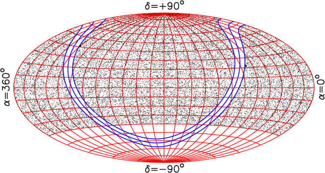
The NVSS (NRAO VLA Sky Survey, Condon et al. 1998) was carried out with the VLA at an observing frequency of 1.4 GHz over the period 1993 – 1996 and covers the whole sky north of declination $-40^{\circ}$ (33,884 square degrees or 82 per cent of the celestial sphere). The source catalogue contains $1.8\times 10^{6}$ sources and is claimed to be 99 per cent complete at integrated flux density $S_{\rm 1.4\,GHz}=3.5$ mJy and 50 per cent complete at 2.5 mJy. These figures are differential completenesses, i.e. 99 per cent of all sources with $S_{\rm 1.4\,GHz}=3.5$ mJy appear in the NVSS catalogue. The survey was performed with the VLA in D configuration, with DnC configuration used for fields at high zenith angles ($\delta<-10^{\circ},\delta>78^{\circ}$), and the FWHM of the synthesized beam is about 45 arc-seconds. The raw fitted source parameters are processed by a computer program provided by the survey team called NVSSlist, which performs the deconvolution and corrects for known biases to produce source diameters and integrated flux densities. Details are given by Condon et al. (1998); NVSSlist version 2.16 (March 2001) was used for this investigation. Figure 1 is a plot of NVSS catalogue entries with $S_{\rm 1.4\,GHz}>200$ mJy.

Figure 1: NVSS catalogue entries with $S_{\rm 1.4\,GHz}>200$ mJy in an equal-area projection. The Galactic plane and Galactic latitudes $\pm 5^{\circ}$ are also plotted; sources within this region are masked from our large-scale structure analysis as many are Galactic in origin.

2.2 FIRST

The FIRST (Faint Images of the Radio Sky at Twenty centimetres) survey, also carried out at an observing frequency of 1.4 GHz but with the VLA in B configuration, began in 1993 and continues. It covers the North and South Galactic caps and the B configuration of the VLA yields an angular resolution of about 5 arcsec. Details of the survey design, analysis and catalogue generation are given in Becker, White & Helfand (1995) and White et al. (1997). These papers claim that the survey is 95 per cent complete at $S_{\rm 1.4\,GHz}=2$ mJy and 80 per cent complete at 1 mJy. These figures are cumulative completenesses, i.e. 95 per cent of sources with $S_{\rm 1.4\,GHz}>2$ mJy appear in the FIRST catalogue.

The latest publicly-available catalogue dates from 15 October 2001. It contains 771,076 sources and covers a total of 8565 square degrees (7954 in the north galactic gap and 611 in the south), or 21 per cent of the celestial sphere. The raw catalogue contains a number of spurious entries representing sidelobe responses from nearby brighter sources. As described in White et al. (1997), the FIRST survey team developed an oblique decision-tree program to identify and flag these sidelobes. In the 15 October 2001 catalogue, 28,017 sources are flagged and were excluded from our analysis.

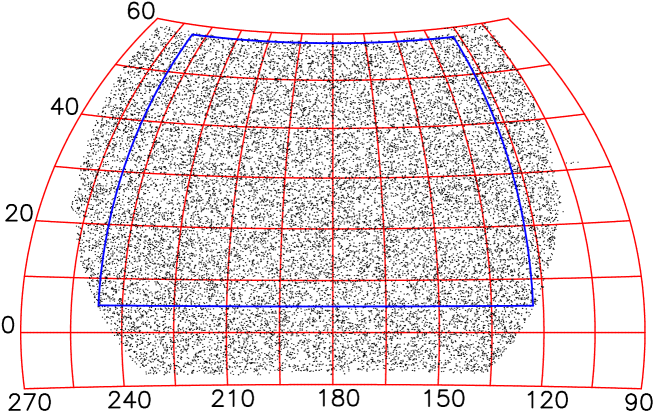
In Figure 2 we plot FIRST catalogue entries with $S_{\rm 1.4\,GHz}>50$ mJy in the northern sky, and we outline the contiguous region for which our large-scale structure analysis was performed ($123^{\circ}<\alpha<247^{\circ}$, $5^{\circ}<\delta<58^{\circ}$).

Figure 2: FIRST catalogue entries with $S_{\rm 1.4\,GHz}>50$ mJy from the 15 October 2001 catalogue, plotted in an equal-area projection. The region for which our large-scale structure analysis was performed ($123^{\circ}<\alpha<247^{\circ}$, $5^{\circ}<\delta<58^{\circ}$) is indicated.

3 Quantifying the angular clustering of galaxies

A common way of quantifying the clustering in an angular distribution of galaxies is by using the angular correlation function, $w(\theta)$. This compares the observed (clustered) distribution to a random (unclustered) distribution of points across the same survey area, by simply measuring the fractional increase in the number of close pairs separated by angle $\theta$. Specifically, if we let $DD(\theta)$ be the number of unique pairs of galaxies with separations $\theta\rightarrow\theta+\delta\theta$, and $RR(\theta)$ be the number of random pairs in the same separation range, then $w(\theta)$ can be estimated as $w(\theta)=(DD-RR)/RR$. Further investigation reveals that the statistical error on $w$ may be minimized by averaging over a large number of random sets ($RR\rightarrow\overline{RR}$) and by using a different estimator for $w$ (see Landy & Szalay 1993). We adopt the Landy-Szalay estimator for our investigations, as this has minimal statistical bias and variance.

Another simple way to quantify the galaxy distribution is to grid the sky into cells of fixed area and shape, and count the number of sources that lie in each cell. Counts-in-cells yields the probability distribution $P(N)$ of finding $N$ sources in a cell, and the moments of the distribution such as the variance $\mu_{2}=\overline{(N-\overline{N})^{2}}$ and skewness $\mu_{3}=\overline{(N-\overline{N})^{3}}$ (the horizontal bar indicates an average over cells). A clustered distribution produces a higher variance than a random distribution because cells may lie in clusters or voids, broadening the probability distribution $P(N)$. Skewness is important because, assuming Gaussian primordial perturbations and linear theory, the skewness of counts-in-cells remains zero (Peebles 1980). Measurement of a non-zero skewness therefore indicates either non-linear gravitational clustering or non-Gaussian initial conditions.

Whereas the angular correlation function bins pair separations into small intervals, a counts-in-cells analysis combines information from a range of angular scales up to the cell size, effectively measuring an average $w(\theta)$ (see equation 1). By avoiding the binning of angular separations, the counts-in-cells is less affected by “shot noise” and is a more sensitive probe of long-range correlations. A simple relation exists between $w(\theta)$ and $\mu_{2}$ ($\S 6.1$), hence we can verify that they are consistent for a given distribution. Neither quantity provides a complete statistical description of the galaxy distribution: this can be encompassed by the hierarchy of correlation functions or the full probability distribution $P(N)$; both are harder to interpret and to compare with theory. Nor are $w(\theta)$ and $\mu_{2}$ well-suited for describing the morphology of the distribution (do galaxies cluster in filaments, sheets or clumps?) or its topology (how do the filaments or sheets join up to form the global pattern?). However, these statistics are easy to measure, provide a simple point of contact with prediction, and can reveal observational problems with the survey data.

4 Observational effects impacting on large-scale structure studies

4.1 Resolution effects

The NVSS and FIRST surveys are at the same observing frequency (1.4 GHz) but at resolutions differing by a factor of 9, and therefore provide an excellent comparative study of survey resolution effects on the observed properties of radio galaxies. In Figure 3 we plot NVSS and FIRST catalogue entries with integrated flux densities $S_{\rm 1.4\,GHz}>3.5$ mJy (at which threshold both surveys are claimed to be complete) in a randomly chosen $3^{\circ}\times 2^{\circ}$ patch of sky. This region contains 230 FIRST entries and 228 NVSS entries. We see that:

• Most radio sources are detected in both surveys.

• Of the objects appearing in just one survey, many more appear in NVSS than FIRST.

• The surface densities are almost identical because many FIRST objects are multiple components of the same galaxy.

Figure 3: NVSS catalogue entries (circles) and FIRST entries (crosses) in a randomly-chosen region of sky common to each survey. We only plot sources with $S_{\rm 1.4\,GHz}>3.5$ mJy, above which threshold both surveys are claimed to be complete.

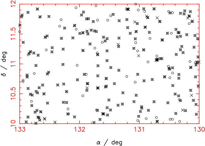
These facts can be explained by the superior angular resolution of FIRST, which picks up multiple radio components unresolved by NVSS. But this high resolution provides FIRST with much poorer sensitivity to surface brightness, losing flux from extended sources even well above the survey limit. Thus the objects appearing solely in NVSS in Figure 3 have fallen below the 3.5 mJy threshold in FIRST. The small number of sources which only appear in FIRST are due to either statistical flux-density errors, source variability, unrecognised sidelobes or noise spikes.

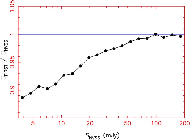
The fact that FIRST under-estimates flux densities is confirmed by Figure 4, which plots the average ratio of FIRST to NVSS integrated flux density for sources matched between the surveys for different NVSS flux-density bands. The matched sources are chosen to be isolated in both surveys (having nearest neighbours more distant than 2 arcmin) to prevent confusion from galaxies resolved as multiple radio components. Figure 4 shows that on average FIRST loses 10 per cent of the flux density from 3.5 mJy sources, a fraction which decreases with increasing flux density.

Figure 4: The average ratio of FIRST to NVSS flux density in NVSS flux-density bands for sources matched between the surveys (with matching tolerance 10 arc-seconds). The matched sources are chosen to be isolated (having nearest neighbours more distant than 2 arcmin) in both surveys to prevent confusion from galaxies resolved into multiple components.

In Figure 5 we overplot differential source counts for FIRST and NVSS for 1 mJy $<S_{\rm 1.4\,GHz}<$ 1 Jy. The curves are in rough agreement. However, the NVSS source count has an unphysical shape below $S_{\rm 1.4\,GHz}\approx 10$ mJy. This distortion arises because NVSSlist uses a different algorithm to convert raw fitted peak amplitudes to integrated flux densities, depending on whether a source is classified as extended or not (Condon et al. 1998). In addition, a larger number of bright ($>100$ mJy) sources are detected in NVSS than in FIRST. This is due to the finer angular resolution of FIRST breaking up bright sources into more radio components.

Figure 5: Differential source counts for NVSS (circles) and FIRST (triangles). The counts are normalized to a Euclidean universe, so that the $y$-axis plots $n(S)\times\,S^{2.5}$ where $n(S)\,dS$ is the number of sources found per steradian in the flux-density range $S\rightarrow S+dS$. The error in each point is smaller than the plotted symbol (except at very high fluxes). At faint flux densities both curves under-estimate the true source count due to incompleteness effects.

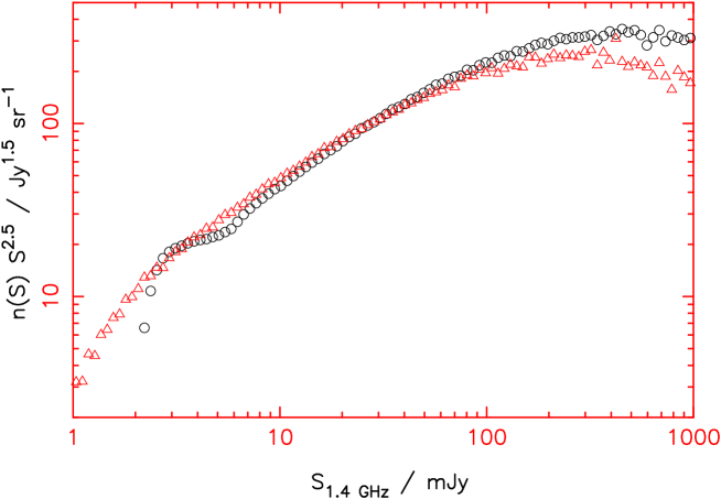
These comparisons demonstrate the significant impact of survey resolution and surface brightness sensitivity on the observed properties of radio galaxies. However, the effect of these flux biases on the deduced large-scale clustering should be minimal: the broadness of the radio galaxy luminosity function ensures that the observed clustering is not a strong function of flux density above 3.5 mJy.

4.2 Gradients in source surface density

Both the NVSS and FIRST surveys suffer from systematic fluctuations in source surface density across the sky above flux-density thresholds at which they are complete, affecting any attempt to quantify the large-scale structure present. Figures 6 and 7 illustrate these variations. In both surveys the magnitude of the effect depends on the flux-density threshold. The FIRST survey contains 10 per cent fluctuations in surface density over the sky at the stated completeness limit $S_{\rm 1.4\,GHz}=2$ mJy, dropping to below 5 per cent at 10 mJy. The variations appear to correlate with the different observing periods. The NVSS suffers from 2 per cent fluctuations at the completeness limit $S_{\rm 1.4\,GHz}=3.5$ mJy, with significant density steps at the declinations where the array configuration is changed from D to DnC, but these fluctuations have become insignificant by 15 mJy. These NVSS effects originate from difficulties in compensating for the sparse $uv$-plane coverage of the survey, constructed from “snapshot” radio observations, and are purely declination-dependent: the projection of array baselines on the sky changes with declination, whereas the data acquisition and analysis software should be insensitive to the right ascension of sources. Note that the NVSS flux-density errors are dominated by a constant additive bias that affects weak sources much more strongly than powerful sources (unlike a multiplicative calibration error).

Figure 6: Variations in NVSS source surface density as a function of declination for sources with integrated flux densities above 3.5 mJy (solid circles) and 15 mJy (open circles). Sources have been binned in declination bands of width $10^{\circ}$. The declination range of each array configuration is also marked on. The error bar on the number of sources $N$ in a band is $\sqrt{N}$. The area within $5^{\circ}$ of the Galactic plane is ignored.

Figure 7: Variations in FIRST source surface density as a function of declination for sources with integrated flux densities above 2 mJy (solid circles) and 10 mJy (open circles). Sources have been binned in declination bands of width $3^{\circ}$; the error bar on the number of sources $N$ in a band is $\sqrt{N}$. The approximate year in which the observations in each declination region were made is also shown.

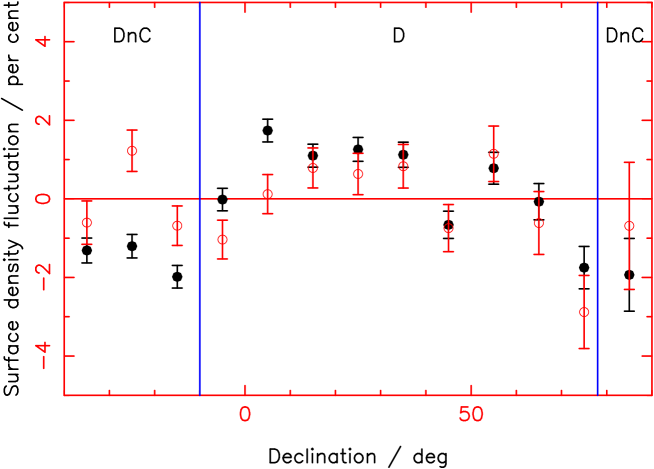
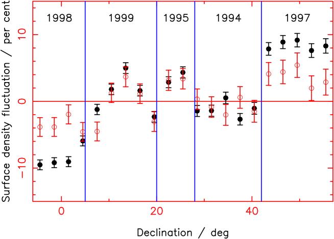
A varying source density $\sigma$ will spuriously enhance the measured value of the angular correlation function $w(\theta)$. This is because the number of close pairs of galaxies in any region depends on the local surface density ($DD\propto\overline{\sigma^{2}}$), but the number of close pairs in the comparison random distribution depends on the global average surface density ($RR\propto(\overline{\sigma})^{2}$). Systematic fluctuations mean that $\overline{\sigma^{2}}>(\overline{\sigma})^{2}$, thus $w(\theta)$ is increased. The variance of counts-in-cells, as quantified by the statistic $y(L)$ (§6.1), will also be increased: a spread in the mean surface density across the cells will inevitably broaden the overall probability distribution $P(N)$, which is constructed from fluctuations about those means. We can show that on angular scales less than those on which $\sigma$ is varying, both $w(\theta)$ and $y(L)$ are subject to the same spurious constant offset $\overline{\delta^{2}}$, where $\delta=(\sigma-\overline{\sigma})/\overline{\sigma}$ is the surface overdensity.

To estimate the magnitude of this effect, take a simple toy model in which a survey is divided into two equal areas between which there is a fractional surface density shift $\epsilon$. For this model, $\overline{\delta^{2}}=\epsilon^{2}/4$. Thus for example the expected offsets on $w(\theta)$ are $\overline{\delta^{2}}\sim 2.5\times 10^{-3}$ for FIRST sources above 2 mJy ($\epsilon\sim 0.1$) and $\overline{\delta^{2}}\sim 2\times 10^{-4}$ for NVSS sources above 3.5 mJy ($\epsilon\sim 0.03$).

In this study, analysis of the radio surveys was restricted to flux-density ranges for which surface gradients were negligible. The alternative approach is to modulate the random comparison sets with the same surface gradients as contained in the data. The gradients are not known in advance and must be measured from the data itself; it was found that this could not be done sufficiently accurately to subtract the offset completely.

4.3 Multiple-component sources

The large linear sizes and complex morphologies of radio sources mean that a single radio galaxy can be resolved in a radio survey (and appear in a survey catalogue) as two or more closely-separated components of radio emission. When investigating the clustering of individual galaxies, these multiple-component sources will produce spurious clustering at small separations. There is no set of criteria that will reliably distinguish multiple-component sources from closely-separated independent galaxies; we instead choose to incorporate their effect into the fitted clustering model. As it turns out, this effect may be successfully disentangled from that of galaxy-galaxy clustering.

The influence of multiple-component sources on the angular correlation function is quantified in detail in our analysis of the NVSS $w(\theta)$ (Blake & Wall 2002), in which it is stressed that even a tiny fraction of giant radio galaxies can substantially affect clustering measurements at small angles. This is because a very small number of close pairs determine the value of $w(\theta)$: we find that we cannot neglect the effect of radio galaxies of size $\theta$ until $\theta\sim 0.1^{\circ}$. At angles $\theta<0.1^{\circ}$, $w(\theta)$ effectively measures the size distribution of radio galaxies; at $\theta>0.1^{\circ}$, the clustering of individual galaxies dominates the pair count. This reasoning is evidenced by the observed numbers and sizes of giant radio sources (Lara et al. 2001) as well as a clear break in the measured $w(\theta)$ at $\theta\approx 0.1^{\circ}$ (see Figure 8). Hence the influence of multiple-component sources may be disentangled from that of galaxy clustering.

At angles where the clustering of individual galaxies dominates the pair count, the fact that these galaxies may be split into multiple radio sources is unimportant. For if the mean number of radio components per galaxy is $\overline{n}$, then the number of pair separations $N_{p}$ at any angle is increased by a factor $(\overline{n})^{2}$, and the source surface density $\sigma$ is increased by a factor $\overline{n}$. As $N_{p}\propto\sigma^{2}\times(1+w)$, the measured correlation function is unaffected.

The effect of multiple-component sources on the moments of counts-in-cells is modelled in Section 6.2.

5 The radio galaxy angular correlation function

5.1 Measurement of the NVSS angular correlation function

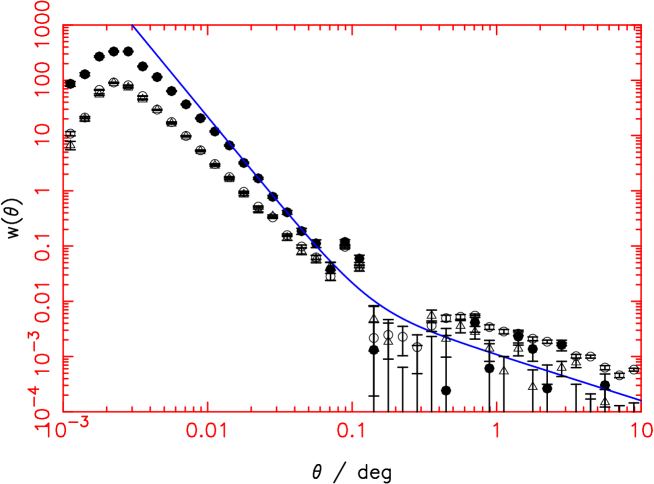
Our measurements of the NVSS $w(\theta)$ for different flux-density thresholds are described in Blake & Wall (2002); the results for 10 mJy and 20 mJy are compared in Figure 8. The angular correlation function at all thresholds can be fit by a sum of two power-laws. A convincing interpretation is that the steep small-angle power-law is created by multiple-component radio sources and hence indicates their size distribution, whereas the shallow large-angle power-law describes the clustering between different radio galaxies.

Figure 8: Measurement of the NVSS angular correlation function for flux-density thresholds $S_{\rm 1.4\,GHz}=20$ mJy (solid circles) and 10 mJy (open circles). The best-fitting sum of two power-laws for the 20 mJy data is overplotted (as are the individual power-laws). The amplitude of the small-angle power-law, which is due to multiple-component sources, decreases with flux-density threshold owing to the increasing surface density (see Blake & Wall 2002). The parameters of the large-angle power-law, which is due to galaxy clustering, are independent of flux-density threshold.

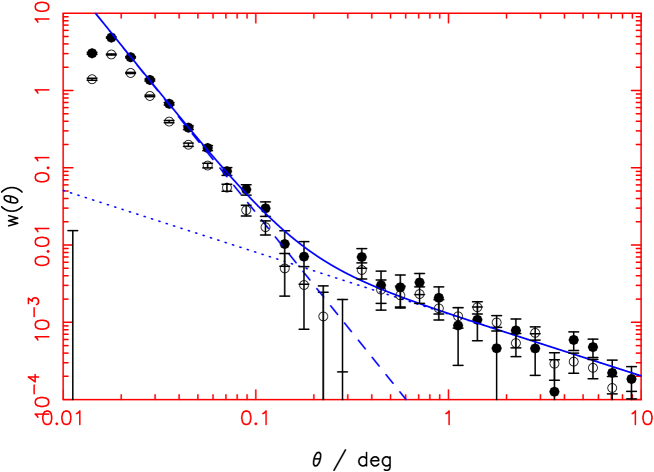
Table 1 displays the results of fitting the function $w(\theta)=A\,\theta^{-\alpha}+B\,\theta^{-\beta}$ to the measurements for flux-density thresholds $S_{\rm 1.4\,GHz}=10,15,20$ mJy. The fits were performed to angles $\theta>0.02^{\circ}$, safely above the resolution limit of the NVSS ($\theta_{{\rm res}}=0.0125^{\circ}$). Figure 8 reveals a fall-off in $w(\theta)$ with decreasing $\theta$ in the lowest separation bins. This is not real, but is a signal-to-noise problem caused by the failure of the survey to resolve weak double sources with separations slightly greater than the beam-width. As $\theta$ increases, a rapidly increasing fraction of doubles of size $\theta$ can be successfully resolved.

Table 1: The best-fitting amplitudes and slopes of the double power-law model $w(\theta)=A\,\theta^{-\alpha}+B\,\theta^{-\beta}$ for the NVSS angular correlation function at different flux-density thresholds; $\theta$ is measured in degrees. The best fit is obtained by minimizing the $\chi^{2}$ statistic. The errors in the parameters are derived by varying each in turn from the best-fitting combination (keeping the others fixed) and determining the variation for which $\Delta\chi^{2}=1$, the appropriate 1-sigma increment when varying one fitted parameter. The value of $\chi^{2}$ is not strictly meaningful given the possible correlations between adjacent separation bins. The reduced $\chi^{2}$ of the best fit and the number of sources $n$ analyzed at each flux-density threshold are also indicated.

$S_{\rm 1.4\,GHz}$	$n$	$A$ / $\times 10^{-3}$	$\alpha$	$B$ / $\times 10^{-5}$	$\beta$	$\chi_{{\rm red}}^{2}$
$>20$	292,962	$1.22\pm 0.15$	$0.76\pm 0.08$	$2.49\pm 0.09$	$3.05\pm 0.01$	1.15
$>15$	375,697	$1.10\pm 0.12$	$0.84\pm 0.07$	$1.62\pm 0.03$	$3.11\pm 0.01$	2.25
$>10$	522,341	$1.08\pm 0.09$	$0.83\pm 0.05$	$0.95\pm 0.02$	$3.18\pm 0.01$	2.24

For all flux-density thresholds, the slope of the clustering power-law is consistent with $\alpha=0.8$ (in agreement with other classes of objects) with an amplitude $A\approx 1\times 10^{-3}$ (with $\theta$ in degrees). Blake & Wall (2002) describe a preliminary analysis of the implications for spatial clustering.

5.2 Comparison with the FIRST angular correlation function

For comparison, we measured $w(\theta)$ from the FIRST catalogue over the region $123^{\circ}<\alpha<247^{\circ}$, $5^{\circ}<\delta<58^{\circ}$ for all objects above flux-density thresholds $S_{\rm 1.4\,GHz}=10$ mJy and 2 mJy. As a precautionary measure, we placed circular masks of radius $0.5^{\circ}$ around all sources with $S_{\rm 1.4\,GHz}>1$ Jy; this left respectively 88,873 and 305,872 objects at the two thresholds. Figure 9 displays the results, compared to the best-fitting NVSS sum of two power-laws at 10 mJy. The FIRST measurement at $\theta\approx 0.1^{\circ}$ is known to be contaminated with sidelobes as described by Cress et al. (1996).

The FIRST 10 mJy and NVSS 10 mJy measurements agree well at small angles, in the regime of multiple-component sources. At bigger angles, the large FIRST error bars mean that $w(\theta)$ is poorly constrained, although the measurement is consistent with the NVSS result ($\chi_{{\rm red}}^{2}=1.84$ for $\theta>0.02^{\circ}$ excluding the two points at $\theta\approx 0.1^{\circ}$). The FIRST 2 mJy $w(\theta)$ measurement has much smaller errors but is offset by the source surface density gradients described in Section 4.2. To verify this, we re-ran the 2 mJy analysis for the more uniform declination region $42^{\circ}<\delta<57^{\circ}$, prompted by Figure 7, using right ascension range $107^{\circ}<\alpha<263^{\circ}$. The re-determined FIRST 2 mJy $w(\theta)$ is in much better agreement with the NVSS result at large angles (see Figure 9). The amplitude of the small-angle FIRST $w(\theta)$ drops between 10 mJy and 2 mJy due to the increased surface density, consistent with the hypothesis that $w(\theta)$ in this regime is entirely governed by multiple-component sources (see Blake & Wall 2002).

Figure 9: Measurements of $w(\theta)$ from the FIRST catalogue. This Figure plots the whole-survey measurements at 10 mJy (solid circles) and 2 mJy (open circles) and the $42^{\circ}<\delta<57^{\circ}$ measurement at 2 mJy (triangles). The solid line is the best-fitting NVSS sum of two power-laws at 10 mJy (see Table 1). The smaller angular resolution of the FIRST survey permits us to explore $w(\theta)$ down to $\theta\approx 0.001^{\circ}\approx 5$ arcsec.

6 Comparison with the radio galaxy counts-in-cells

We also performed a counts-in-cells analysis of the radio surveys. Our motivation was twofold: to quantify the clustering imprint with an independent statistic to compare with $w(\theta)$, and to make contact with previous work (Magliocchetti et al. 1998, 1999).

6.1 Relation of counts-in-cells variance to $w(\theta)$

Consider an unclustered distribution of sources, distributed randomly and independently with surface density $\sigma$. The expected number of sources in a cell of area $S$ is $<N>=\sigma\times S$. The expected probability distribution $P(N)$ is the Poisson distribution with mean $<N>$ and variance $<N>$. We define the following statistic to quantify the increased variance of a clustered distribution:

$$y=\frac{\mu_{2}-\overline{N}}{(\overline{N})^{2}}$$

Hence $<y>=0$ for no clustering, as $<\mu_{2}>=<\overline{N}>=<N>$. (Actually, as there is statistical error in the denominator, $y$ contains a slight bias which may be neglected). We can show (Peebles 1980, equation 36.6) that for a given $w(\theta)$, the expected value of $y$ is

$$<y>=\frac{\int_{{\rm cell}}\int_{{\rm cell}}w(\theta)\,dS_{1}\,dS_{2}}{S^{2}}=\int w(\theta)\,\frac{dG_{p}}{d\theta}d\theta$$ (1)

where in the final expression, $dG_{p}$ is the fraction of all pairs of area elements within the cell lying in the separation range $\theta\rightarrow\theta+d\theta$ (using the notation of Landy & Szalay 1993). $dG_{p}$ may be calculated analytically for simple geometries:

• For a square of side $L$, putting $x=\theta/L$,

  $$\frac{dG_{p}}{dx}=\cases{2x\,(\pi-4x+x^{2})&$0\leq x\leq 1$\cr 2x\,[\pi-2+4\sqrt{x^{2}-1}-4\arccos{(1/x)}-x^{2}]&$1\leq x\leq\sqrt{2}$\cr}$$ (2)

• For a circular cell of diameter $L$, putting $x=\theta/L$,

  $$\frac{dG_{p}}{dx}=\frac{16\,x}{\pi}\left(\arccos{(x)}-x\sqrt{1-x^{2}}\right)$$ (3)

We now calculate $<y>$ for a power-law angular correlation function. If the survey has angular resolution $\theta_{{\rm res}}$ then

$$w(\theta)=\cases{-1&$\theta<\theta_{{\rm res}}$\cr(\theta/\theta_{0})^{-\alpha}&$\theta>\theta_{{\rm res}}$\cr}$$

Hence from equation 1,

$$<y>=-\int_{0}^{\theta_{{\rm res}}}\frac{dG_{p}}{d\theta}\,d\theta+\int_{\theta_{{\rm res}}}^{\theta_{{\rm max}}}\left(\frac{\theta}{\theta_{0}}\right)^{-\alpha}\,\frac{dG_{p}}{d\theta}\,d\theta$$

where $\theta_{{\rm max}}=L$ for a circular cell of diameter $L$ and $\theta_{{\rm max}}=L\sqrt{2}$ for a square cell of side $L$. To unveil the clustering pattern we measure the variation of $<y>$ with cell size $L$, for fixed cell shape. This is elegantly done by the substitution $x=\theta/L$:

$$<y(L)>=-\int_{0}^{\theta_{{\rm res}}/L}\frac{dG_{p}}{dx}\,dx+\left(\frac{\theta_{0}}{L}\right)^{\alpha}\int_{\theta_{{\rm res}}/L}^{x_{{\rm max}}}x^{-\alpha}\,\frac{dG_{p}}{dx}\,dx$$ (4)

The quantity $dG_{p}/dx$ is determined purely by the cell shape, not size (see equations 2 and 3). For small $x$, $dG_{p}/dx=kx$ independently of cell shape ($k=8$ for circular cells and $k=2\pi$ for square cells). Assuming that $\theta_{{\rm res}}\ll L$, this solves the first integral of equation 4:

$$<y(L)>=-\frac{k}{2}\left(\frac{\theta_{{\rm res}}}{L}\right)^{2}+\left(\frac{\theta_{0}}{L}\right)^{\alpha}\int_{\theta_{{\rm res}}/L}^{x_{{\rm max}}}x^{-\alpha}\,\frac{dG_{p}}{dx}\,dx$$

• If the slope of $w(\theta)$ is steep enough ($\alpha>2$), the non-Poisson clustering will be dominated by close pairs ($x\ll 1$) and for all cell shapes we can neglect edge effects by assuming that $dG_{p}/dx=kx$ and $x_{{\rm max}}=\infty$. This allows us to solve the second integral of equation 4 and obtain:

  $$<y(L)>=k\left(\frac{\theta_{{\rm res}}}{L}\right)^{2}\left[\frac{1}{(\alpha-2)}\left(\frac{\theta_{0}}{\theta_{{\rm res}}}\right)^{\alpha}-\frac{1}{2}\right]$$ (5)

• Otherwise, cell shape is important and the exact solution is

  $$<y(L)> = k\left(\frac{\theta_{{\rm res}}}{L}\right)^{2}\left[\frac{1}{(\alpha-2)}\left(\frac{\theta_{0}}{\theta_{{\rm res}}}\right)^{\alpha}-\frac{1}{2}\right]$$ (6)

  $$+ \left(\frac{\theta_{0}}{L}\right)^{\alpha}\left[\int_{x_{{\rm min}}}^{\infty}x^{-\alpha}\frac{dG_{p}}{dx}dx-\frac{k}{(\alpha-2)x_{{\rm min}}^{\alpha-2}}\right]$$

  where $x_{{\rm min}}=\theta_{{\rm lim}}/L_{{\rm min}}$, and the integral must be solved numerically.

Thus equation 6 shows that in general, $<y>$ has a variation with cell size of the form

$$<y(L)>=a\,L^{-2}+b\,L^{-\alpha}$$ (7)

where $a$ and $b$ are constants. The limited angular resolution $\theta_{{\rm res}}$ reduces the variance: the existence of an object in a cell limits the available space in which other objects can appear. This effect varies with cell size because it depends on the scale of the resolution relative to the cell size. If a survey has sharp enough angular resolution then the first term of equation 7 may be neglected (if $\alpha<2$), and $<y>\propto L^{-\alpha}$. This is the case for the FIRST survey but not for the NVSS; thus equation 9 of Magliocchetti et al. (1998) only contains the second term of our equation 7.

The following statistic is commonly defined to characterize the departure of the skewness from a Poisson distribution:

$$z=\frac{\mu_{3}-3\mu_{2}+2\overline{N}}{(\overline{N})^{3}}$$ (8)

This has the expectation value

$$<z>=\frac{\int_{{\rm cell}}\int_{{\rm cell}}\int_{{\rm cell}}W(\theta_{12},\theta_{13},\theta_{23})\,dS_{1}\,dS_{2}\,dS_{3}}{S^{3}}$$

where $W(\theta_{12},\theta_{13},\theta_{23})$ is the three-point angular correlation function. The significance of the skewness is summarized in Section 3 above.

6.2 Effect of multiple-component sources on the counts-in-cells moments

The existence of multiple-component sources increases the moments of counts-in-cells. This is because the fraction of radio sources within a cell that are split into multiple components varies from cell to cell, which acts to broaden the probability distribution of counts-in-cells. The simplest model is to suppose that a fraction $e$ of the galaxies are double sources (i.e. two sources appearing at the same location in space) and a fraction $f$ are triple sources. It can be shown (Blake 2002) that the expected offsets in the variance and skewness statistics are

$$\Delta y=\frac{1}{\sigma\,S}\left(\frac{2e+6f}{1+e+2f}\right)$$ (9)

$$\Delta z=\frac{1}{(\sigma\,S)^{2}}\left(\frac{6f}{1+e+2f}\right)$$ (10)

where $S$ is the cell area and $\sigma$ is the surface density of all components (i.e. catalogue entries). Thus skewness is sensitive only to triple sources.

This simple model neglects the fact that the components of a radio galaxy have a range of non-zero separations, but this should only matter if the cell size is not much greater than the maximum component separation ($\sim 0.1^{\circ}$). A more sophisticated treatment is to model the separation distribution by the effective (small-angle) $w(\theta)$ of Figure 8. We can compute the effect on the variance statistic $y$ using equation 7, thus the general expression for $y(L)$ can be modified to

$$<y(L)>=a\,L^{-2}+b\,L^{-\alpha}+c\,L^{-\beta}$$

where $c$ is a constant and $\alpha$ and $\beta$ are respectively the slopes of the shallow (galaxy clustering) and steep (multiple component) $w(\theta)$ power-laws.

It is easy to show that this more sophisticated model reduces in the appropriate limit to the more simple treatment initially outlined. As component separations tend to zero, the slope $\beta$ of the effective $w(\theta)$ becomes large and we can use the “steep clustering” approximation of equation 5, which reproduces the dependence $y\propto L^{-2}$ of equation 9.

6.3 Error on the counts-in-cells moments

Variance and skewness measurements are subject to statistical error due to averaging over a finite number of cells $N_{c}$. Calculating the standard error on the statistics $y$ and $z$ in the case of a random (unclustered) distribution yields

$$\sigma_{y}=\sqrt{\frac{2}{N_{c}\,(\overline{N})^{2}}}$$ (11)

$$\sigma_{z}=\sqrt{\frac{6}{N_{c}\,(\overline{N})^{3}}}$$ (12)

The probability distribution of the clustered data does not depart greatly from a Poisson distribution ($y\ll 1$, $z\ll 1$), so that these expressions are very good approximations to the actual statistical errors.

6.4 Measuring the counts-in-cells moments from a real survey

To measure the counts-in-cells we used the simple technique of defining a grid of touching circular cells of diameter $L$ on the sky and counting the number of sources that fall inside each cell. This only utilises a fraction $\pi/4$ of the available area, but the cell shape is constant over the sky. We note that the methodology of counts-in-cells was revolutionized by Szapudi (1998) who showed that it was valid to throw a very large number of randomly-placed cells over the sky, heavily oversampling the survey area. We prefer the former, simpler approach for a first investigation aiming to show consistency with the $w(\theta)$ analysis.

Surveys do not encompass the whole sky: there are boundaries and masked regions. Hence some cells in the grid are partially filled, the $i$th cell having fraction of useful area $f_{i}$ (say). To determine $f_{i}$ for each cell we populated the sky with random points subject to the same boundaries and masks as the real survey. Counting the number of random points that fall in each cell accurately measures the useful area. We then boosted the data count in the $i$th cell by a factor $1/f_{i}$, unless $f_{i}$ was less than a threshold $f_{{\rm rej}}=0.75$ in which case we rejected the cell. To measure the factors $f_{i}$ accurately enough it is essential to average over a sufficiently large number of random realizations that statistical noise does not dominate. Let there be $m$ random sets, each with the same surface density as the survey. The lower limit on $m$ is determined by the following considerations:

• The correction of cell counts by factors $1/f_{i}$ creates extra variance in the counts-in-cells (because all cells are corrected, whether they are partially filled or not). This extra systematic variance must be much smaller than the statistical error of equation 11. This condition is equivalent to

  $$m\gg m_{1}=\sqrt{\frac{N_{c}}{2}}\left(1+\frac{1}{\overline{N}}\right)$$

• The cell areas must be determined precisely enough that a negligible fraction of “unspoilt” cells are rejected with $f_{i}<f_{{\rm rej}}$. This condition is equivalent to

  $$m\gg m_{2}=\frac{1}{\overline{N}\,(1-f_{{\rm rej}})^{2}}$$

When evaluating the moments of the counts-in-cells distribution we assume that all cells are populated independently. This is not strictly true given that clustered sources have correlated positions, but the assumption should be a very good approximation if the cells are large enough. With this consideration in mind, we adopted a minimum cell size $L_{{\rm min}}=0.3^{\circ}$ for our analysis; below this cell size the average number of sources contained in a cell drops below $\overline{N}=1$ at the relevant flux-density thresholds.

6.5 Measurement of the NVSS counts-in-cells moments

Using these methods, we measured the counts-in-cells variance statistic $y(L)$ from the NVSS for circular cells of diameters $0.3^{\circ}<L<10^{\circ}$ for flux-density thresholds $S_{\rm 1.4\,GHz}=10$ mJy and 20 mJy. As described in Blake & Wall (2002), we masked out all NVSS catalogue entries within $5^{\circ}$ of the Galactic plane and also within 22 additional masked regions around radio sources that appear in the NVSS catalogue as a large number of separate elliptical Gaussians. As discussed in Section 5.1, the difficulty in resolving faint doubles with separations just greater than the beam-width causes some variation in the effective survey angular resolution, as evidenced by the fall-off in $w(\theta)$ with decreasing $\theta$ in the lowest separation bins of Figures 8 and 9. To ensure a consistent value of $\theta_{{\rm res}}$ for the prediction of the counts-in-cells variance from $w(\theta)$, we ran a linking algorithm that combined together all pairs of sources with angular separations less than 1 arcmin, thus artificially establishing $\theta_{{\rm res}}=1$ arcmin. This left 289,981 NVSS catalogue entries above 20 mJy and 516,782 entries above 10 mJy.

The variance measurements at the two flux-density thresholds are plotted in Figure 10, with error bars from equation 11. We also plot the predictions generated from the double power-law model for $w(\theta)$ with best-fit coefficients at the appropriate flux-density thresholds as listed in Table 1. The counts-in-cells variance is visually consistent with the prediction of the measured angular correlation function, verifying the agreement of these two independent methods of quantifying angular structure in the NVSS. The $\chi^{2}$ statistics between the data and the prediction are $\chi_{{\rm red}}^{2}=0.69$ at 20 mJy and $\chi_{{\rm red}}^{2}=1.64$ at 10 mJy. However, the value of $\chi^{2}$ is not strictly meaningful because the variances for different cell sizes are not independent. Note that multiple-component sources produce an approximately constant offset in $y\,L^{2}$ in Figure 10. The variance statistic for the 10 mJy threshold falls below that for the 20 mJy measurement because this offset is proportional to $1/\sigma$, where $\sigma$ is the source surface density (see equation 9).

Figure 10: The NVSS counts-in-cells variance statistic $y(L)$ is plotted for thresholds 20 mJy (solid circles) and 10 mJy (open circles) together with the predictions of the double power-law $w(\theta)$ model at 20 mJy and 10 mJy (the solid lines). The dashed and dotted lines show the separate contributions to $y(L)$ at 20 mJy of the steep (multiple-component) $w(\theta)$ and shallow (galaxy clustering) $w(\theta)$. The angular correlation function predictions provide a good fit to the measurements of the variance, demonstrating the consistency of these independent methods of quantifying angular structure in the NVSS.

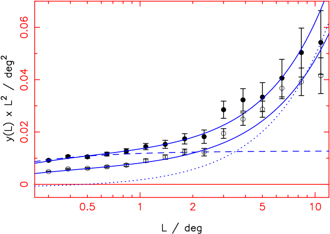
The angular correlation function model used to generate the predictions is a sum of two power-laws, representing respectively multiple-component sources ($w(\theta)\propto\theta^{-3.1}$) and galaxy clustering ($w(\theta)\propto\theta^{-0.8}$). To assess the contribution of each effect to the overall counts-in-cells variance we separately converted each of the two 20 mJy power-laws to a variance and plotted the result on Figure 10. For small cell sizes ($L<1^{\circ}$) the extra variance produced by multiple-component sources dominates. For larger cell sizes the extra variance produced by galaxy clustering becomes increasingly important. This type of transition is expected, as the number of extra pairs at angle $\theta$ scales as $w(\theta)\times 2\pi\theta\,d\theta$, which varies as $\theta^{-2.1}$ for multiple-component sources and $\theta^{+0.2}$ for pairs of galaxies.

By converting the measured $w(\theta)$ into an equivalent variance we have shown that the angular correlation function and counts-in-cells analyses are entirely consistent. Alternatively, we can make an independent determination of the angular correlation function parameters by finding the best fit to $y(L)$. We varied the amplitude and slope of the clustering power-law $w(\theta)=A\,\theta^{-\alpha}$, whilst keeping the multiple-component $w(\theta)$ parameters fixed at their best-fitting values from Table 1. Thus for each point in the $(A,\alpha)$ grid we obtained a model $y(L)$, which we compared with the measured $y(L)$ using the $\chi^{2}$ statistic. The best-fitting clustering parameters were in good agreement with those derived from the original $w(\theta)$ analysis (see Figure 11).

Figure 11: Constraints on the clustering parameters $w(\theta)=A\,\theta^{-\alpha}$ from counts-in-cells. The angular correlation function may be converted into a variance of counts-in-cells (Section 6.1) and thereby compared with the counts-in-cells measurements. Multiple components are modelled as a second power-law $w(\theta)$, the coefficients of which are held constant at their best-fitting values (Table 1). The Figure shows $1\sigma$ and $2\sigma$ contours in the space of $(A,\alpha)$ for flux-density thresholds of 10 mJy (solid) and 20 mJy (dashed). As the plot is in the space of two varying parameters, these contours are defined by $\chi^{2}$ increasing by respectively 2.30 and 6.17 from its minimum, although as variance measurements for different cell sizes are not independent, the value of $\chi^{2}$ is not strictly meaningful.

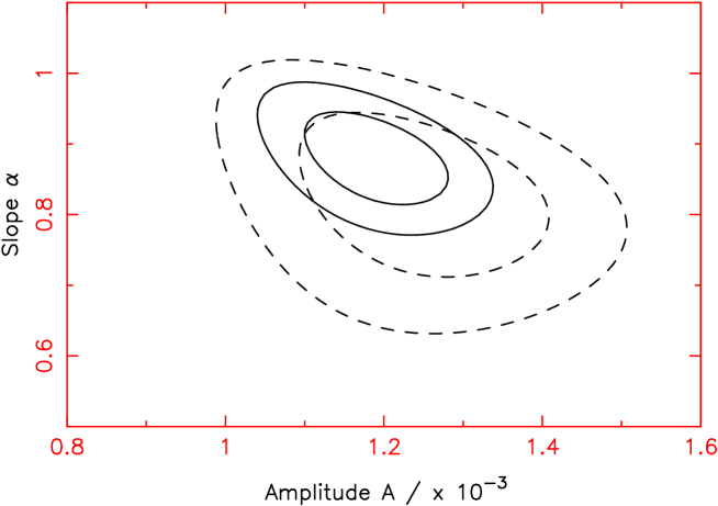
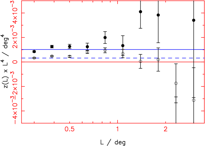
Figure 12 displays measurements of the skewness statistic $z(L)$ (equation 8) from the NVSS at 20 mJy and 10 mJy. The result is a significant detection of skewness. However, the fact that $z$ scales roughly as $L^{-4}$ suggests that the skewness is dominated by multiple-component sources, especially as the amplitude of the skewness scales with surface density in accordance with equation 10. On Figure 12 we plot the multiple-component skewness predictions at 10 mJy and 20 mJy assuming that 7 per cent of radio galaxies are doubles (see Blake & Wall 2002) and 1 per cent are triples (i.e. $e=0.07$, $f=0.01$). This fraction of triple sources is reasonable; analyzing NVSS sources into groups using link-length $\theta_{{\rm link}}=5$ arcmin (a reasonable approximation to the range of dominance of multiple-component sources, see Figure 8) produces groups of which 9.8 per cent are doubles and 1.5 per cent are triples. These skewness predictions due to multiple components produce a fairly good fit to the data. The NVSS hence provides no convincing evidence for cosmological skewness.

Figure 12: Measurement of the NVSS skewness statistic $z(L)$ for thresholds 20 mJy (solid circles) and 10 mJy (open circles). The prediction of the multiple-component model of equation 10 is also plotted for 20 mJy (solid line, $\sigma=9.37$ deg^-2) and 10 mJy (dashed line, $\sigma=16.69$ deg^-2) assuming a fraction of doubles $e=0.07$ and triples $f=0.01$. The skewness statistic becomes dominated by noise for cell sizes $L>1^{\circ}$ due to the decreasing number of cells contained in the grid. It is most convenient to plot $z\times L^{4}$ against $L$ to illustrate the influence of multiple components.

6.6 Comparison with the FIRST counts-in-cells variance

We also derived counts-in-cells for the FIRST radio survey, previously studied by Magliocchetti et al. (1998). Our results are not directly comparable to those of Magliocchetti et al. (1998) as we make no attempt to combine multiple-component sources. We analyzed the three FIRST sub-samples used in the angular correlation function study of Section 5.2. To ensure a consistent survey angular resolution we first ran the source-combining algorithm with link-length $\theta_{{\rm res}}=0.003^{\circ}$.

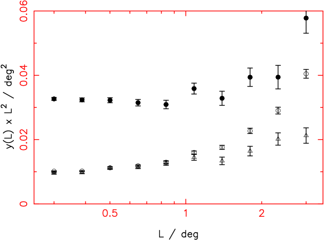
The variance results for the three FIRST sub-samples are plotted in Figure 13. In all samples there is a strong contribution from multiple components ($y\,L^{2}=$ constant) which dominates at small cell sizes. The amplitude of this contribution varies as $1/\sigma$ where $\sigma$ is the source surface density (equation 9), which accounts for the overall shift between the 10 mJy and 2 mJy samples (between which $\sigma$ varies by a factor $\approx 3.4$). Angular resolution effects are unimportant for FIRST; hence there is no dip in the variance at small $L$. Galaxy clustering becomes important at higher $L$ ($y\propto L^{-\alpha}$). The difference between the two samples at 2 mJy arises from the surface density gradients present in the whole-sky sample. Gradients offset the counts-in-cells variance by $\Delta y=$ constant (Section 4.2), as is apparent from the increasing difference between the plotted triangles and open circles in Figure 13 (which plots $y\,L^{2}$ against $L$). Comparing Figures 13 and 10, the greater angular resolution of FIRST with respect to NVSS leads to an increased abundance of multiple-component sources and thus a greater variance signal for a given flux-density threshold.

Figure 13: The FIRST counts-in-cells variance $y(L)$ is plotted for the three samples defined in the text: 10 mJy all-sky (solid circles), 2 mJy all-sky (open circles) and 2 mJy reduced area (triangles). The errors in the data points are determined using equation 11.

6.7 Comparison with previous work

Our results differ from those of Magliocchetti et al. (1998) in two respects:

1. Magliocchetti et al. (1998) reported a much steeper slope for the correlation function, $\gamma=2.5\pm 0.1$ (where $w(\theta)\propto\theta^{1-\gamma}$) compared to our NVSS measurement $\gamma=1.83\pm 0.05$ (Table 1). Magliocchetti et al. adopted a combining algorithm for multiple components and assumed that, after the operation of this algorithm, any remaining pairs were independent radio galaxies. However, no set of criteria can unequivocally distinguish multiple components from independent galaxies, and a small number of residual multiple-component sources can have a dramatic effect on the clustering statistics on angular scales up to several arc-minutes (see Blake & Wall 2002). As demonstrated by Figure 8, multiple components are the dominant provider of close pairs in the NVSS up to $\theta\approx 0.1^{\circ}$, whereas the fraction of closely-separated pairs combined by Magliocchetti et al. becomes negligible by $0.02^{\circ}$. Thus the steep slope found by Magliocchetti et al. may be a manifestation of the remaining multiple-component sources, and not of galaxy clustering. Furthermore, it is difficult to understand a steep slope $\gamma=2.5$ persisting to small angles, given that the $\gamma\approx 1.8$ clustering law is obeyed by all other studied classes of galaxy including local optically-selected galaxies (both spirals and ellipticals, e.g. Loveday et al. 1995) and high-redshift QSOs (Croom et al. 2001).

2. Magliocchetti et al. (1998) reported a cosmological skewness. We suggest that this may also be produced by uncombined doubles. The relation $z\propto y^{2}$ used by Magliocchetti et al. as evidence for the non-linear gravitational growth of perturbations (their equation 20) is also naturally produced in a model where multiple components dominate – it results from combining our equations 9 and 10. An alternative explanation lies in the different flux-density limits (10 mJy for NVSS versus 3 mJy for FIRST). The FIRST sample may contain a non-negligible fraction of low-redshift starburst galaxies which trace non-linear clustering and hence are a source of skewness.

7 Conclusions

We have quantified the angular clustering in the NVSS and FIRST radio surveys using two independent methods: the two-point angular correlation function and the variance on counts-in-cells. Our results may be summarized as follows:

1. The results of angular correlation function and counts-in-cells analyses of the surveys are entirely consistent.

2. The larger area and greater number of sources in the NVSS yield a much clearer description of the clustering imprint. The correlation function has two contributions: that due to multiple components of the same galaxy, dominant at $\theta<0.1^{\circ}$, and that due to clustering between galaxies, which dominates at larger angles. A clear break in $w(\theta)$ is evident between these scales. Both of these contributions are needed to explain the observed variance on counts-in-cells.

3. The clustering part of the correlation function has a slope consistent with that measured in the optical regime, $w(\theta)\propto\theta^{-0.8}$; this is confirmed by our counts-in-cells measurements.

4. Both the NVSS and FIRST surveys suffer from systematic fluctuations in source surface density at flux-density thresholds at which they purport to be complete.

Our work disagrees with some previous conclusions drawn from the FIRST survey:

1. We find a galaxy correlation slope consistent with that measured in the optical, $\gamma\approx 1.8$, in contrast to somewhat steeper slopes reported in previous analyses. These steeper slopes may have been produced by residual multiple component radio sources.

2. The skewness reported by Magliocchetti et al. (1998) may also be due to these residual double sources.

This investigation has improved our understanding of the methodology of angular clustering analyses for large-scale radio surveys, of relevant observational effects present in such surveys, and of the derived structural parameters. There is now the basis to use these surveys to derive three-dimensional information on the very largest structural scales, adopting more powerful statistical methods in conjunction with the redshift databases to be provided by surveys such as 2dF and SDSS.

References

- [1] Baleisis A., Lahav O., Loan A.J., Wall J.V., 1998, MNRAS, 297, 545
- [2] Becker R.H., White R.L., Helfand D.J., 1995, ApJ, 450, 559
- [3] Bhavsar S., Barrow J., 1983, MNRAS, 205, 61
- [4] Blake C.A., 2002, PhD thesis, University of Oxford
- [5] Blake C.A., Wall J.V., 2002, MNRAS, 329, L37
- [6] Chiang L., Coles P., 2000, MNRAS, 311, 809
- [7] Condon J.J., Cotton W.D., Greisen E.W., Yin Q.F., Perley R.A., Taylor G.B., Broderick J.J., 1998, AJ, 115, 1693
- [8] Cress C.M., Helfand D.J., Becker R.H., Gregg M.D., White R.L., 1996, ApJ, 473, 7
- [9] Cress C.M., Kamionkowski M., 1998, MNRAS, 297, 486
- [10] Croom S.M., Shanks T., Boyle B.J., Smith R.J., Miller L., Loaring N.S., Hoyle F., 2001, MNRAS, 325, 483
- [11] Kooiman B.L., Burns J.O., Klypin A.A., 1995, ApJ, 448, 500
- [12] Krzewina L., Saslaw W., 1996, MNRAS, 278, 869
- [13] Landy S.D., Szalay A.S., 1993, ApJ, 412, 64
- [14] Lara L., Cotton W.D., Feretti L., Giovannini G., Marcaide J.M., Marquez I., Venturi T., 2001, A&A, 370, 409
- [15] Loan A.J., Wall J.V., Lahav O., 1997, MNRAS, 286, 994
- [16] Loveday J., Maddox S.J., Efstathiou G., Peterson B.A., 1995, ApJ, 442, 457
- [17] Maddox S.J., Efstathiou G., Sutherland W.J., 1996, MNRAS, 283, 1227
- [18] Magliocchetti M., Maddox S.J., Lahav O., Wall J.V., 1998, MNRAS, 300, 257
- [19] Magliocchetti M., Maddox S.J., Lahav O., Wall J.V., 1999, MNRAS, 306, 943
- [20] Peebles P.J.E., 1980, The Large-Scale Structure of the Universe, Princeton Univ. Press, Princeton, NJ
- [21] Rengelink R.B., Miley G.K., Rottgering H.J.A., Bremer M.N., de Bruyn A.G., Tang Y., 1998, in Observational Cosmology with the New Radio Surveys, Kluwer Academic Publishers, p.143
- [22] Szapudi I., 1998, ApJ, 497, 16
- [23] White R., Becker R., Helfand D., Gregg M., 1997, ApJ, 475, 479