Stellar Structure Modeling using a Parallel Genetic Algorithm for Objective Global Optimization

Abstract

Genetic algorithms are a class of heuristic search techniques that apply basic evolutionary operators in a computational setting. We have designed a fully parallel and distributed hardware/software implementation of the generalized optimization subroutine PIKAIA, which utilizes a genetic algorithm to provide an objective determination of the globally optimal parameters for a given model against an observational data set. We have used this modeling tool in the context of white dwarf asteroseismology, i.e., the art and science of extracting physical and structural information about these stars from observations of their oscillation frequencies. The efficient, parallel exploration of parameter-space made possible by genetic-algorithm-based numerical optimization led us to a number of interesting physical results: (1) resolution of a hitherto puzzling discrepancy between stellar evolution models and prior asteroseismic inferences of the surface helium layer mass for a DBV white dwarf; (2) precise determination of the central oxygen mass fraction in a white dwarf star; and (3) a preliminary estimate of the astrophysically important but experimentally uncertain rate for the ${}^{12}{\rm C}(\alpha,\gamma)^{16}{\rm O}$ nuclear reaction. These successes suggest that a broad class of computationally-intensive modeling applications could also benefit from this approach.

1 Astrophysical Context

About 5 billion years from now, the hydrogen fuel in the center of the Sun will begin to run out and the helium that has collected there will begin to gravitationally contract, increasing the rate of hydrogen burning in a shell surrounding the core. Our star will slowly bloat into a red giant—eventually engulfing the inner planets, perhaps even the Earth. As the helium core continues to contract under the influence of gravity, it will eventually reach the temperatures and densities needed to fuse three helium nuclei into a carbon nucleus (the $3\alpha$ reaction). Another nuclear reaction will compete for the available helium nuclei at the same temperature: the carbon can fuse with an additional helium nucleus to form oxygen. The amount of oxygen produced during this process is largely determined by the relative rates of these two competing reactions [1]. Since the Sun is not very massive by stellar standards, it will never get hot enough in the center to produce nuclei much heavier than carbon and oxygen. These elements will collect in the center of the star, which will then shed most of its red giant envelope—creating a planetary nebula—and emerge as a hot white dwarf star [2].

Once a white dwarf star forms and the nuclear reactions have ceased, its structural and thermal evolution is dominated by cooling, and regulated by the opacity of its thin atmospheric outer layers. It will slowly fade as it radiates its residual thermal energy into space—eventually cooling through a narrow range of temperatures that will cause it to vibrate in a periodic manner, sending gravity-driven seismic waves deep through the interior and bringing information to the surface in the form of brightness variations. This is fortunate, because a detailed record of the nuclear history of the star is locked inside, and pulsations provide the only known key to revealing it.

We can determine the internal composition and structure of pulsating white dwarfs using the techniques of high speed photometry to observe their variations in brightness over time, and then matching these observations with a computer model which behaves the same way. The observational aspects of this procedure have been addressed by the development of the Whole Earth Telescope (WET) network [3], a group of astronomers at telescopes around the globe who cooperate to produce nearly continuous time-series photometry of a single target for 1-2 weeks at a time. The Fourier spectra of such observations reveal dozens of excited modes with periods in the range 100–1000 seconds, supporting our interpretation of them as non-radial oscillations with gravity as the restoring force ($g$-modes). The WET has now provided a wealth of seismological data on the different varieties of pulsating white dwarf stars.

The physical property of white dwarf models that most directly determines the pulsation frequencies is the radial profile of the Brunt-Väisälä (buoyancy) frequency, which is given by

$$N^{2}=-g\left({d\ln\rho\over dr}-{1\over\Gamma_{1}}{d\ln P\over dr}\right),$$ (1)

where $g$ is the local gravity, $\rho(r)$ the density, $P(r)$ the pressure, and $\Gamma_{1}$ is $(\partial\ln P/\partial\ln\rho)$ at constant entropy. The magnitude of $N^{2}$ reflects the difference between the actual and the adiabatic density gradients, and sets the local propagation speed of internal gravity waves. The observed frequencies, in turn, are a measure of the average (inverse) wave speed in the portion of the interior where the waves propagate. Inferring the $N^{2}$ internal profile from the observed pulsation frequencies is thus a classical inverse problem, on par in scope and complexity with similar problems encountered in helio- and geo-seismology.

Consider first the complementary forward problem, which consists in computing the oscillation frequencies of a given white dwarf structural model. The forward modeling procedure begins with a static, non-rotating, unmagnetized, spherically symmetric model of a pre-white dwarf, which we allow to evolve quasi-statically until it reaches the desired surface temperature. The models must initially satisfy two of the basic equations of stellar structure: the condition of hydrostatic equilibrium, which balances the outward pressure gradient against the inward pull of gravity

$${dP\over dr}={GM_{r}\over r^{2}}\rho\ ,$$ (2)

and the continuity equation ensuring mass conservation

$${dM_{r}\over dr}=4\pi r^{2}\rho\ ,$$ (3)

where $M_{r}$ is the mass contained within a spherical shell of radius $r$. White dwarf stars are compact objects supported mainly by electron degeneracy pressure ($P_{e}$), and we can describe the core with a simple polytropic equation of state of the form

$$P_{e}\propto\left({\rho\over\mu_{e}}\right)^{5/3},$$ (4)

where $\mu_{e}$ is the mean molecular weight per free electron. Cooling is achieved by leaking the internal thermal energy through the opacity of the thin atmospheric layers at a rate consistent with the star’s luminosity, and adjusting the interior structure accordingly. Although we initially ignore a third equation of stellar structure (which ensures thermal balance), we do use it to evolve the models in a self-consistent manner. The cooling tracks of our polytropic models quickly forget the unphysical initial conditions and converge with the evolutionary tracks of self-consistent pre-white dwarf models well above the temperatures at which the hydrogen- and helium-atmosphere white dwarfs are observed to be pulsationally unstable [4].

Next, the $g$-mode pulsation frequencies ($\sigma_{g}$) of the evolved models must be calculated for comparison with the observations. Working in the usual spherical polar coordinates $(r,\theta,\phi)$, the first step is to express the radial displacement ($\Xi_{r}$) experienced by an oscillating fluid element as

$$\Xi_{r}(r,\theta,\phi,t)=\xi_{r}(r)Y_{\ell}^{m}(\theta,\phi)\exp(i\sigma_{g}t)~{},$$ (5)

where the $Y_{\ell}^{m}$ are the usual spherical harmonic functions [5]. For a given set of angular and azimuthal quantum numbers $(\ell,m)$, the linearized adiabatic non-radial oscillation equations reduce to a one-dimensional linear eigenvalue problem for $\sigma_{g}$ and $\xi_{r}$, described by the following set of equations:

$$\frac{1}{r^{2}}\frac{d}{dr}(r^{2}\xi_{r})-\frac{g}{c_{s}^{2}}\xi_{r}+\left(1-\frac{L_{\ell}^{2}}{\sigma_{g}^{2}}\right)\frac{P^{\prime}}{\rho c_{s}^{2}}=\frac{\ell(\ell+1)}{\sigma_{g}^{2}r^{2}}\Phi^{\prime},$$ (6)

$$\frac{1}{\rho}\frac{dP^{\prime}}{dr}+\frac{g}{\rho c_{s}^{2}}P^{\prime}+(N^{2}-\sigma_{g}^{2})\xi_{r}=-\frac{d\Phi^{\prime}}{dr},$$ (7)

$$\frac{1}{r^{2}}\frac{d}{dr}\left(r^{2}\frac{d\Phi^{\prime}}{dr}\right)-\frac{\ell(\ell+1)}{r^{2}}\Phi^{\prime}=4\pi G\rho\left(\frac{P^{\prime}}{\rho c_{s}^{2}}+\frac{N^{2}}{g}\xi_{r}\right),$$ (8)

where $\Phi^{\prime}$ is the perturbation of the gravitational potential, $c_{s}$ is the sound speed, $L_{\ell}^{2}\equiv\ell(\ell+1)c_{s}^{2}/r^{2}$ is the Lamb or acoustic frequency, and $\xi_{r}$ is the (small) radial displacement associated with a given mode of frequency $\sigma_{g}$ (see [6] for a detailed derivation). The eigenmodes associated with a given set of $(\ell,m)$ values possess radial harmonics which can be labeled with a third quantum number ($k$) related to the number of nodes in the corresponding radial eigenfunction, so that the frequencies of individual eigenmodes are best labeled as $\sigma_{k\ell m}$.

Inverting a continuous function, in our case $N^{2}(r)$, from a discrete set of data (the pulsation periods) is well known to be a mathematically ill-posed problem [7, 8]. However, the situation is not as critical as one might imagine because strong physical constraints can be placed on the variations with depth of the Brunt-Väisälä frequency. In white dwarf interiors, the $N^{2}(r)$ profile is determined by the structural stratification (e.g., variations of density and pressure with depth), which in turn depends on the star’s evolutionary history as well as a number of physical parameters such as stellar mass, core chemical composition, surface temperature, and the mass of its surface helium layer, to name but a few. The ill-posed inverse problem for $N^{2}$ can be then recast in the form of an optimization problem that consists in finding the numerical values for the set of these parameters that yields the optimal fit between the oscillation periods of the corresponding white dwarf structural model, as computed via the forward procedure outlined above, and the observed periods. From the point of view of numerical optimization, this is now a well-posed problem.

With detailed observations and a theoretical model in hand, the next step is to select a suitable numerical optimization method. Models of all but the simplest physical systems are typically non-linear, so finding the optimal match to the observations requires an initial guess for each parameter. Some iterative method is generally used to improve on this first guess until successive iterations do not produce significantly different answers. There are at least two potential problems with this standard approach to model-fitting. The first guess is often derived from the past experience of the person who is fitting the model. This subjective method is even worse when combined with a local approach to iterative improvement. Many optimization schemes, such as differential corrections [9] or the simplex method [10], yield final results that depend to some extent on the choice of initial model parameters. This does not have serious consequences if the parameter-space contains a single, well-defined minimum. But if there are many local minima, then it can be more difficult for a traditional approach to find the globally optimal solution (e.g., see Fig. 1 of [11]).

The multi-modal nature of the optimization problem is not the only modeling pitfall to be reckoned with. A good fit between model periods and data certainly suggests that the model adequately reflects the actual physical structure of the stars themselves. However, the possibility can never be ruled out that other physical characteristics of the white dwarf models, considered known and held fixed in the present modeling work, could also be varied to yield comparably good fits to the observed frequencies. As with any inverse problem, asteroseismic inferences are plagued by the potential for non-uniqueness of the solutions. With this caveat firmly in mind, we proceed.

2 Genetic Algorithms

An optimization scheme based on a genetic algorithm (GA) can avoid the problems inherent in many traditional approaches. The range of possible values for each parameter is restricted only by observations and by the constitutive physics of the model. Although the parameter-space defined in this way is often quite large, a GA provides a relatively efficient means of searching globally for the optimal model. Although it is more difficult for GAs to find precise values for the optimal set of parameters efficiently, they are well suited to search for the region of parameter-space that contains the global minimum. In this sense, the GA is an objective means of obtaining a good first guess for a more traditional local hill-climbing method, which can narrow in on the precise values and uncertainties of the optimal solution.

Genetic algorithms [12, 13, 14, 15], arguably still the most popular class of evolutionary algorithms [16, 17], were inspired by Charles Darwin’s notion of biological evolution through natural selection [18]. The basic idea is to solve an optimization problem by evolving the global solution, starting with an initial set of purely random guesses. The evolution takes place within the framework of the model, with the individual parameters serving as the genetic building blocks. Selection pressure is imposed by some goodness-of-fit measure between model and observations. Several books have been written to describe how these ideas can be applied in a computational setting [12, 13], but we provide a basic overview below.

To begin, the GA samples the parameter-space at a fixed number of points defined by a uniform selection of randomly chosen values for each parameter. The GA evaluates the model for each set of parameters, and the predictions are compared to observations. Each point in the “population” of trials is subsequently assigned a fitness based on the relative quality of the match. A new generation of sample points is then created by selecting from the current population of points according to their computed fitness, and then modifying their defining parameter values with two genetic operators in order to explore new regions of parameter-space.

Rather than modifying the parameter values directly, the genetic operators are applied to encoded representations of the parameter sets. The simplest way to encode them is to convert the numerical values of the parameters into a string of digits. The string is analogous to a chromosome, and each digit is like a gene. For example, a point defined by two parameters with numerical values $a_{1}=0.123$ and $b_{1}=0.456$ could be encoded into the string 123456.

The two basic genetic operators are crossover, which emulates sexual reproduction, and mutation which emulates somatic defects. The crossover procedure pairs up the strings, chooses a random position for each pair, and swaps the two strings from that position to the end. For example, suppose that the encoded string above is paired with another point having $a_{2}=0.567$ and $b_{2}=0.890$, which encodes to the string 567890. If the second position between numbers on the string is chosen, the strings become:

$${\tt 12}\framebox{\tt 3456}\rightarrow{\tt 12}\framebox{\tt 7890}$$ (9)

$${\tt 56}\framebox{\tt 7890}\rightarrow{\tt 56}\framebox{\tt 3456}$$ (10)

To help keep favorable combinations of parameters from being eliminated or corrupted too hastily, this operation is not applied to all of the pairs. Instead, it is assigned a fixed occurrence probability ($p_{c}$) per selected pair.

The mutation operator spontaneously replaces a digit in the string with a new randomly chosen value. In our above example, if the mutation operator is applied to the fourth digit of the second string, the result might be

$${\tt 563}\framebox{\tt 4}{\tt 56}\rightarrow{\tt 563}\framebox{\tt 2}{\tt 56}$$ (11)

Such digit replacement occurs with a small probability ($p_{m}$), often dubbed the mutation rate.

After both operators have been applied, the strings are decoded back into sets of numerical values for the parameters. In this example, the new first string 127890 becomes $a^{\prime}_{1}=0.127$ and $b^{\prime}_{1}=0.890$, and the new second string 563256 becomes $a^{\prime}_{2}=0.563$ and $b^{\prime}_{2}=0.256$. Note that mutation in this case has caused a significant “jump” in parameter-space, from the value $b^{\prime}_{2}=0.456$ that would have been generated by the crossover operation only. The new genetically-shuffled set of points replaces the original set, and the process is repeated until some termination criterion is met.

What is the justification for this rather contorted way to produce two new trial points from two existing ones? One could have instead simply formed the arithmetic averages of the pairs $a_{1},a_{2}$, and $b_{1},b_{2}$. However, under the “pressure” of fitness-based selection, crossover acting on successive generations of strings modifies the frequency of a given substring in the population at a rate proportional to the difference between the mean fitness of the subset of strings incorporating that substring, and the mean fitness of all strings making up the current population. This mouthful is given quantitative expression in the so-called schema theorem [12, 14, 15], which continues to form the basis of most theoretical analysis of GAs. The GA can be thought of as a classifier system that continuously sorts out and combines the most advantageous substrings that happen to be present across the whole population at a given time. In this context the role of mutation is to inject “novelty” continuously, by producing new digit values at specific string positions, which might not otherwise have been present in the population or may have been selected against during earlier evolutionary phases.

It should be clear already from this brief introductory discussion that the operation of a GA involves a number of random processes, so that the resulting search algorithm is stochastic in nature. Consequently, there is always a finite probability that the GA will not find the globally optimal solution in a given run. This probability decreases gradually, of course, as the evolution is pushed through more and more generations. Alternately, one can run the GA for fewer generations, but do so several times with different random initialization. This form of higher-level Monte Carlo simulations makes it possible to establish the validity of the optimal set of model parameters with an acceptable degree of confidence.

3 The PIKAIA subroutine

PIKAIA is a self-contained, genetic-algorithm-based optimization subroutine developed at the High Altitude Observatory, and available in the public domain (http://www.hao.ucar.edu/public/research/si/pikaia/pikaia.html). PIKAIA maximizes a user-specified FORTRAN function through a call in the body of the main program. Unlike many GA packages available commercially or in the public domain, PIKAIA uses decimal (rather than binary) encoding. This choice was motivated by portability issues—binary operations are usually carried out through platform-dependent functions in FORTRAN, which makes it more difficult to port the code between PC and workstation platforms. While originally designed primarily as a learning tool, PIKAIA’s portability, ease of use, and robustness have made it by all appearances the software of choice for a wide variety of modeling problems requiring global optimization capabilities (see [19, 20, 21, 22] for sample applications; and the PIKAIA web page for a compilation of past and present users and their research applications).

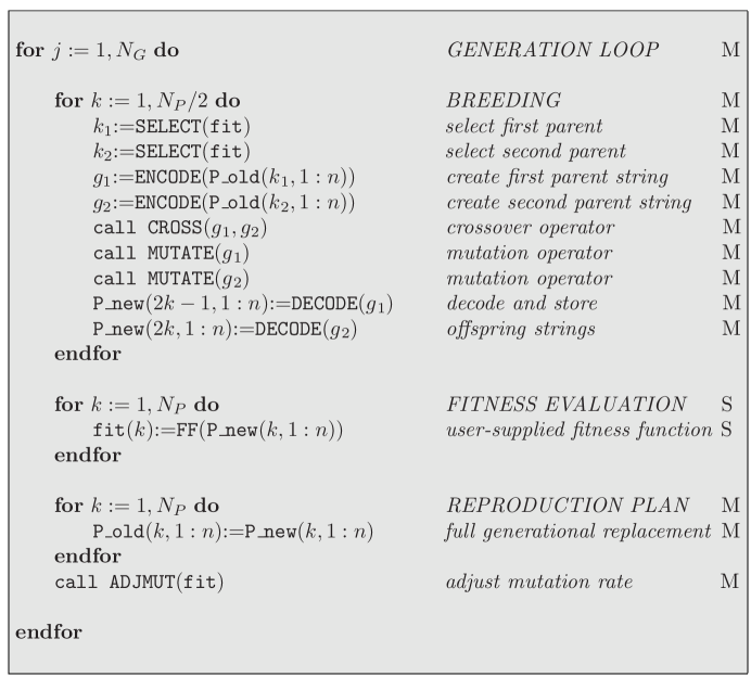
Figure 1:  Minimal pseudo-code for the PIKAIA genetic algorithm optimization subroutine, operating in Full-Generational-Replacement mode. The number of model parameters being optimized is $n$, $N_{P}$ is the (fixed) population size, and $N_{G}$ is the number of (time-like) generations over which the evolution is carried out. The functions ENCODE and DECODE convert a $n$-dimensional floating-point array to a string, and vice-versa. The function SELECT picks a single individual (flagged by an integer, here $k_{1}$ or $k_{2}$), with a probability proportional to its fitness-based rank in the current population. Note that the strings $g_{1}$, $g_{2}$ are modified upon exit from CROSS and MUTATE, and since each breeding event produces two offspring, the first inner loop only needs to repeat $N_{P}/2$ times to produce a new, full-size population. Operations and function calls labeled “M” are carried out serially by the Master program, and those labeled “S” are executed in parallel by the Slave processes (see §4 for more details).

3.1 GA structure: Select-Breed-Evaluate-Replace

Fig. 1 shows, in pseudo-code form, the algorithmic structure of PIKAIA. The inner workings of the various functions and subroutines appearing therein have been described at length elsewhere [11, 23], and so are only outlined in what follows. We do describe in some detail in §3.2 and §3.3 below additional strategies and operators not originally included in the public-release version PIKAIA 1.0.

The task at hand is the maximization of the user-supplied function FF, which accepts as input an $n$-dimensional floating-point array x($1:n$) containing a set of parameter values defining one instance of the model being optimized, and returning a measure of goodness-of-fit (based, e.g., on a $\chi^{2}$ measure if the model output is being compared to data). The code evolves a population of $N_{P}$ trial points in the $n$-dimensional search space, stored in the array P_old($1:N_{P},1:n$), through a preset number of generations $N_{G}$. The population is (usually) initialized with random deviates uniformly distributed in user-specified intervals defining the range of parameter-space to be explored, so that the evolutionary search remains bounded but otherwise entirely unbiased by the choice of initial conditions.

At each time-like generation (outer loop), pairs of “parents” are extracted from the current population, with selection probability increasing with the individual’s fitness, using a rank-based version of the classical Roulette Wheel Algorithm [13]. The two corresponding $n$-dimensional floating-point arrays are then encoded into two strings ($g_{1},g_{2}$), bred using crossover and mutation operators, and decoded back into two $n$-dimensional floating-point arrays that define the two “offspring” points. These are stored in the temporary array P_new, which concludes the breeding step. The fitness of the new population members is then computed via the user-supplied fitness function FF, and stored in the $N_{P}$-dimensional array fit. Finally, a reproduction plan is needed to insert some or all of the newly generated and evaluated trial points into the breeding population. The simplest strategy, dubbed “Full-Generational-Replacement”, consists in breeding a number of new trial points equal to that within the original population (first inner loop, repeating only $N_{P}/2$ times since each breeding event produces two offspring), and then replacing the old population with the new (third inner loop). This concludes one generational iteration, and the above steps are repeated anew.

3.2 Dynamical adjustment of the mutation rate

Of the various internal parameters governing the operation of the genetic algorithm itself, the mutation rate is one that often sensitively affects performance [12, 17]. This rate is more aptly defined as the probability ($0\leq p_{m}\leq 1$) that a single digit in the encoded strings will be subjected to replacement by another random digit, as already described briefly in §2. As with biological systems, mutation is very much a mixed blessing. It represents the only way to inject variability into the evolving population [14], which is extremely useful—some would say essential—for efficient exploration of parameter-space and displacement of the population away from secondary extrema. But too much mutation can also destroy the existing good solutions. Some sort of optimal tradeoff between these incompatible tendencies must be achieved by a proper choice of $p_{m}$.

Various “recipes” for setting $p_{m}$ have been put forth, starting with simple prescriptions such as setting $p_{m}=(N_{P}L)^{-1}$, where $L$ is the string length [24], detailed empirical modeling [25], all the way to meta-simulations where a higher-level GA evolves the combination of controlling parameters that yields the best performance of the underlying GA for the problem under consideration [26]. However, near-optimal performance is rarely sustained across wide ranges of problems. Moreover, because of the very large number of model evaluations involved, some of the more elaborate approaches rapidly become impractical if the modeling problem at hand is very computation intensive, as is the case with the problem considered here.

One way around this quandary is to allow $p_{m}$ to vary dynamically in the course of an evolutionary run, according to the degree of clustering of the current population as a whole. The public-release version of PIKAIA does so by monitoring the normalized difference ($\Delta$) between the fitness values of the best and median individuals in the population (ranking being based on fitness):

$$\Delta={\max({\tt fit})-{\rm med}({\tt fit})\over\max({\tt fit})+{\rm med}({\tt fit})},\qquad[{\rm fitness~{}based}].$$ (12)

A strongly clustered (scattered) population has $\Delta\to 0$ ($\Delta\to 1$). At the end of each generational iteration, $\Delta$ is computed, and if found to fall below (exceed) a preset lower (upper) bound $\Delta_{1}$ ($\Delta_{2}$), the mutation rate is multiplicatively incremented (decremented) by a factor $\delta$:

$$p_{m}\to\cases{p_{m}\times\delta,&$\Delta\leq\Delta_{1}$,\cr p_{m}/\delta,&$\Delta\geq\Delta_{2}$.\cr}$$ (13)

Experience reveals that the GA’s performance is not sensitively dependent on the adopted values for $\Delta_{1},\Delta_{2}$ and $\delta$, within reasonable bounds. Numerical values $\Delta_{1}=0.05$, $\Delta_{2}=0.25$, $\delta=1.5$ have proved to be robust over a variety of test problems, and are hardwired in PIKAIA’s mutation rate adjustment subroutine (ADJMUT in Fig. 1).

Clearly, Eq. (12) is not the only possible measure of population clustering. Another possibility is to use a measure of metric distance between the best and median individual in the population:

$$\Delta^{2}={1\over n}\sum_{k=1}^{n}(x_{k}^{\rm max}-x_{k}^{\rm med})^{2}\qquad[{\rm distance~{}based}],$$ (14)

where $x_{k}^{\rm max}$ ($x_{k}^{\rm med}$) represents the $k^{\rm th}$ element of the $n$-dimensional floating-point array containing the parameter values defining the current best (median) individual in the population. Which of Eqs. (12), (14) will yield the best optimization performance cannot be foretold, as the answer will depend on the shape of the fitness isosurface in parameter-space (and if these are known a priori in detail, then the optimization problem is already solved!). On synthetic white dwarf data, distance-based adjustment was found to increase the success rate (i.e., probability of locating the true global optimum) of the search process by $\sim$50% over fitness-based adjustment, all other GA control parameters being the same (see Fig. 2).

Dynamical adjustment of $p_{m}$ can lead to relatively large mutation rates in some evolutionary phases, with the potential danger of destroying good solutions. PIKAIA avoids this by making use of a small but very useful “cheat” known as elitism [24], which saves the fittest member of the breeding population (P_old) and recopies it to the new population (P_new) as the final step of the reproduction plan.

PIKAIA’s dynamical adjustment of the mutation rate represents a particularly simple form of self-adaptation (see [27], and articles therein). PIKAIA can function anywhere along a spectrum extending between two very qualitatively distinct search modes; as long as $p_{m}\ll 1$, PIKAIA operates as a classical genetic algorithm, with the crossover operator primarily responsible for the exploration of parameter-space. On the other hand, as $p_{m}\to\Delta_{2}$ PIKAIA behaves more and more like a stochastic iterated hill-climber. This peculiar algorithmic combination has proven to be both robust and efficient.

Figure 2:  Sample convergence curves for GA runs using different methods for dynamical adjustment of the mutation rate. The top panel shows the variance of the best trial in the population as a function of generation using distance-based adjustment with (solid) and without (dashed) creep mutation included, and using fitness-based adjustment with creep mutation (dotted). The bottom panel shows the corresponding mutation rate as a function of generation for the three methods. Crossover is primarily responsible for the initial rapid improvement in all three curves. Both distance-based curves converge to the global solution, though more slowly when creep mutation is included. The fitness-based method is much less successful escaping local minima, but eventually converges to the region of the global solution.

3.3 Creep mutation

The one-point mutation operator included in the public-release version of PIKAIA suffers from a well-known shortcoming, which may prove troublesome under certain problem-dependent circumstances. Consider the following portion of a string encoding a parameter value $a=0.1961$:

$${\tt...1961...}$$ (15)

Assume now that the optimal solution has $a^{\ast}=0.2050$, and that the search space is smooth enough that, at least early in the evolution, an individual with $a=0.1961$ has above-average fitness. The occurrence frequency of the above substring in the population will increase, and sequential action of one-point mutation is likely to lead to a gradual trend toward the substring

$${\tt...1999...}$$ (16)

But now we have a problem. Going from this substring to the optimal 2050 requires some simultaneous and well-coordinated digit substitutions on the part of one-point mutation, which, statistically, are highly unlikely. The string has become stuck at a so-called “Hamming wall”.

Encoding schemes can be designed such that successive single digit changes in the string translate into smooth variations of the decoded parameter values. Binary Gray coding [16, 28] is a well-known example. An alternate, often more practical solution is to make use of a new mutation operator known as creep mutation [13]. In the context of decimal encoding, this would operate as follows. Rather than randomly replacing a digit targeted for mutation, add or subtract $1$ (with equal probabilities) to the existing digit, and “carry over the one” when appropriate. For example,

$${\tt...19}\framebox{\tt 9}{\tt 9...}\rightarrow{\tt...1}\framebox{\tt 90}{\tt 9...}\rightarrow{\tt...}\framebox{\tt 100}{\tt 9...}\rightarrow{\tt...2009...}.$$ (17)

Clearly creep mutation can cross Hamming walls, but it lacks the ability to generate occasional large “jumps” in parameter-space the way one-point mutation can if it operates on a string element that decodes into a leading digit in the corresponding floating-point parameter. Since this latter property is advantageous for exploration of parameter-space, whenever carrying out mutation (call MUTATE in Fig. 1), it is preferable to pick either one-point or creep mutation with equal probabilities.

The use of creep mutation for our white dwarf modeling problem gave mixed results; it led to a higher probability of finding the exact set of optimal parameters, but at the expense of slightly slower convergence to the region of the global solution (see Fig. 2). This probably reflects the fact that there were no Hamming walls in the vicinity of the optimal solution. In other PIKAIA applications, however, creep mutation has been found to lead to significant improvements. As with so many other aspects of GA-based numerical optimization, the benefit of creep mutation is highly problem-dependent.

4 Parallel Implementation

In 1998 we began a project to adapt some well-established white dwarf evolution and pulsation codes to interface with PIKAIA. On the fastest processors available at the time, a single model would run in about 45 wallclock seconds. Knowing that the optimization would require $\sim$10^5-6 models, it was clear that a serial version of PIKAIA would require many months to finish on a single processor. So we decided to incorporate the message passing routines of the Parallel Virtual Machine (PVM) software [29] into PIKAIA.

4.1 General parallelization considerations

The PVM software allows a collection of networked computers to cooperate on a problem as if they were a single multi-processor parallel machine. All of the software and documentation is free. We had no trouble installing it on our Linux cluster [30] and the sample programs that come with the distribution made it easy to learn and use. The trickiest part of the procedure was deciding how to split up the workload among the various computers.

Figure 3:  The scalability of the parallel version of PIKAIA on a 64-node Linux cluster using the white dwarf fitness function. The cluster contains two types of CPUs (PIII and K6-2) running at slightly different speeds (300 and 366 MHz), but the points in this plot were produced using equal numbers of each, scaled relative to the average performance of the two types.

The GA-based fitting procedure for the white dwarf code quite naturally divided into two basic functions: evolving and pulsating white dwarf models, and applying the genetic operators to each generation once the fitnesses had been calculated. When we profiled the distribution of execution time for each part of the code, this division became even more obvious. Here, as with the vast majority of real-life applications, fitness evaluation (second inner loop on Fig. 1) is by far the most computationally demanding step. For our model-fitting application, 93% of CPU time is spent carrying out fitness evaluation, 4% carrying out breeding and GA internal operations (such as mutation rate adjustment), and 3% for system and I/O. It thus seemed reasonable to create a slave program to perform the model calculations, while a master program took care of the GA-related tasks.

In addition to decomposing the function of the code, a further division based on the data was also possible. Fitness evaluation across the population is inherently a parallel process, since each model can be evaluated independently of the others. Moreover, it requires minimal transfer of information, since all that the user-supplied function FF requires is the $n$-dimensional floating-point array of parameters defining one single instance of the model, and all it needs to return is the floating-point value corresponding to the model’s fitness. It is then natural to send one model to each available processor, so the number of machines available would control the number of models that could be calculated in parallel. Maximal use of each processor is then assured by choosing a population size $N_{P}$ that is an integer multiple of the number of available processors.

In practice, this recipe for dividing the workload between the available processors proved to be very scalable. Since very little data is exchanged between the master and slave tasks, our 64-node cluster provided a speedup factor of about 53 over the performance on a single processor (see Fig. 3).

4.2 Master Program

Starting with the slightly improved unreleased version of PIKAIA, including creep mutation and distance-based mutation rate adjustment, we used the message passing routines from PVM to create a parallel fitness evaluation subroutine. The original code evaluated the fitnesses of the population one at a time in a DO loop (equivalent to the second inner loop in Fig. 1). We replaced this procedure with a single call to a new subroutine that evaluates the fitnesses in parallel on all available processors. The parallel version of PIKAIA constitutes the master program, which runs on the central computer of our Linux cluster. A flow chart for the parallel fitness evaluation subroutine (PVM_FITNESS.F) is shown in Fig. 4.

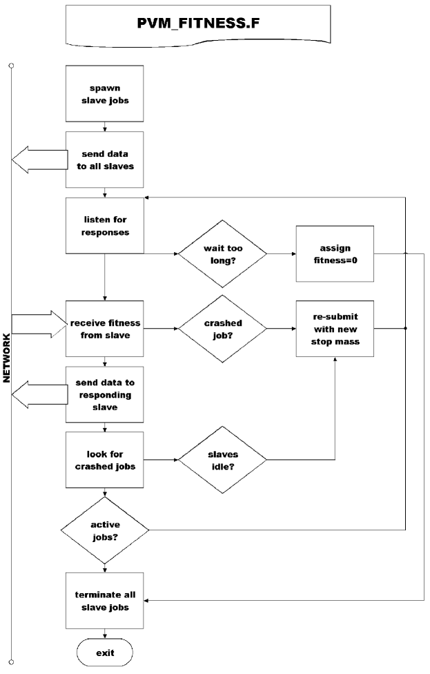
Figure 4:  Flow chart for the parallel fitness evaluation subroutine, which runs on the master computer.

After starting the slave program on every available processor, PVM_FITNESS.F sends an array containing scaled values of the parameters to each slave job over the network. In the first generation of the GA, these values are completely random; in subsequent generations, they are the result of the selection, crossover, and mutation of the previous generation, performed by the non-parallel portions of PIKAIA.

Next, the subroutine listens for responses from the network and sends a new set of parameters to each slave job as it finishes the previous calculation. When all sets of parameters have been sent out, the subroutine begins looking for jobs that may have crashed and re-submits them to slaves that have finished and would otherwise sit idle. If a few jobs do not return a fitness after an elapsed time much longer than the average runtime required to compute a model, the subroutine assigns them a fitness of zero. In a typical run, this was necessary for less than 1 in 10,000 model evaluations. When every set of parameters in the generation have been assigned a fitness value, the subroutine returns to the main program to perform the genetic operations—resulting in a new generation of models to calculate. The process continues for a fixed number of generations, chosen to maximize the success rate of the search.

In all simulation runs reported below, we kept the crossover probability fixed at $p_{c}=0.85$, used an initial mutation probability $p_{m}=0.005$, and retained a level of selection pressure corresponding to PIKAIA’s default settings. We determined the optimal number of generations by applying the method to synthetic data and looking at the fraction of runs that converged to the input model as a function of run length, up to 500 generations. To minimize the probability of missing the global solution for observed data, we fixed the number of generations to be slightly larger than the test run that converged the slowest. Within the range of control parameters we explored, our GA application exhibited a clear tradeoff effect between population size $N_{P}$ and number of generational iterations $N_{G}$. As long as the product $N_{P}N_{G}$ remained near $3\times 10^{4}$, the success probability of a single GA run was approximately constant at $\sim$70%.

4.3 Slave Program

The original white dwarf code came in three pieces: (1) the evolution code, which starts with a static polytropic approximation of a pre-white dwarf and allows it to cool quasi-statically until it reaches the desired temperature, (2) the prep code, which reformats the output of the evolution code, and (3) the pulsation code, which uses the output of the prep code to solve the adiabatic non-radial oscillation equations, yielding the mode periods to be compared with the observed periods.

To get the white dwarf code running in an automated way, we merged the three components of the original code into a single program, and added a front end that communicated with the master program through PVM routines. This code (FF_SLAVE.F) combined with the fitness function constitutes the slave program, and is run on each node of the Linux cluster. A flow chart for FF_SLAVE.F is shown in Fig. 5.

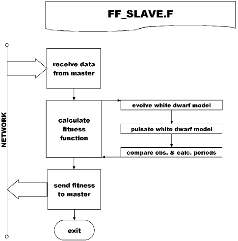
Figure 5:  Flow chart for the slave program of the parallel code, which runs on each node of the Linux cluster.

The operation of the slave program is relatively simple. Once it is started by the master program, it receives a set of parameters from the network. It then calls the fitness function (the white dwarf code in our case) with these parameters as arguments. Our fitness function rescales the dimensionless parameters into physical units, and cools a polytropic white dwarf model with the proper mass and structure down to the specified temperature. A typical model has several hundred spherical mass shells, and requires at most a few dozen time steps to cool down to the relevant temperatures.

The slave program then calculates the adiabatic non-radial pulsation periods within a specified range, given the spherical degree of the modes (only $\ell\leq 2$ have been observed in white dwarfs). This involves solving Eqs. (6)–(8), which is carried out numerically using an iterative scheme based on the Runge-Kutta-Fehlberg shooting method [31]. The first guess for the eigenvalue can be obtained from the following useful approximation of the $g$-mode pulsation frequencies:

$$\sigma_{k\ell m}\approx\left<{N^{2}\ell(\ell+1)\over k^{2}r^{2}}\right>^{1/2}+\left(1-{C_{k}\over\ell(\ell+1)}\right)m\Omega$$ (18)

where the second term is due to the slow rotation frequency $\Omega$ (which breaks the spherical symmetry), and the constant $C_{k}$ is of order unity [32]. Typically, only a few iterations are needed to achieve convergence on a radial mesh with several thousand effective zones, where the model quantities are interpolated by means of a cubic spline between the equilibrium model shells, equally spaced in mass.

Finally, each of the observed periods ($P_{\rm obs}$) are compared to the nearest model periods ($P_{\rm mod}$), and the variance ($\sigma$) is calculated,

$$\sigma=\left({1\over N}\sum_{j=1}^{N}(P_{\rm obs}-P_{\rm mod})^{2}\right)^{1/2}~{},$$ (19)

with $N=11$ for the data used here. The fitness is then defined as the inverse of this root-mean-square period residual, and is sent to the master program over the network. The node is then ready to run the slave program again and receive a new set of parameters from the master program.

5 Results

The ultimate goal of our project was to derive a measurement of the astrophysically important ${}^{12}{\rm C}(\alpha,\gamma)^{16}{\rm O}$ nuclear reaction rate. When a white dwarf star is being formed in the core of a red giant during helium burning, the $3\alpha$ and ${}^{12}{\rm C}(\alpha,\gamma)^{16}{\rm O}$ reactions compete for the available helium nuclei. The relative rates of the two reactions determines the final yield of oxygen deep in the core. The $3\alpha$ rate is well established, but the same is not true of the ${}^{12}{\rm C}(\alpha,\gamma)^{16}{\rm O}$ reaction. The extrapolation of its rate to stellar energies from high-energy laboratory measurements is complicated by interference between various contributions to the total cross-section, leading to a relatively large uncertainty [33]. This translates into similarly large uncertainties in our understanding of every astrophysical process that depends on this reaction, from supernovae explosions to galactic chemical evolution. A seismological measurement of the core oxygen mass fraction $X_{\rm O}$ in a pulsating white dwarf star can provide an independent way to determine the ${}^{12}{\rm C}(\alpha,\gamma)^{16}{\rm O}$ reaction at stellar energies.

Knowledge of the central oxygen mass fraction has other important astrophysical implications. Surveys of white dwarfs in our galactic neighborhood have demonstrated a marked deficit at luminosities below about $10^{-6}$ times the solar luminosity ($L_{\odot}$) [34]. The favored interpretation is that even the oldest white dwarfs in the galaxy have not yet had time to cool below the observed cutoff luminosity [35]. This opened the possibility to infer the age of the galactic disk, and thus obtain a lower limit on the age of the Universe. White Dwarf Cosmochronometry, as the subject has been called, evidently requires detailed knowledge of the white dwarf thermal energy content and cooling history [36]. The former turns out to depend significantly on the core chemical composition, primarily the mass ratio of carbon-to-oxygen ($X_{\rm C}/X_{\rm O}$), these being the two constituents that theoretically account for the near totality of the core mass.

Our first application of the parallel GA allowed only 3 parameters to be varied in the models: the surface temperature, the stellar mass, and the thickness of a surface helium layer. To the extent possible, we defined the boundaries of the search using only observational constraints and limits imposed by the underlying physics. It was the broadest survey of white dwarf pulsation models ever conducted, covering more than 100 times the search volume of previous studies. After demonstrating that the method was successful on synthetic data, we applied it to the best-observed star among the helium-atmosphere pulsators, GD 358, using data obtained by the Whole Earth Telescope [3]. The original analysis of these data [37] identified a series of eleven ($\ell=1,m=0$) pulsation modes of consecutive radial overtone ($k=8$–18) with periods between 400 and 900 seconds. The measured trigonometric parallax of GD 358 confirmed this $\ell$ identification beyond doubt, since the luminosity of models with higher $\ell$ modes could not be reconciled with this independent constraint. The initial asteroseismic study of GD 358 from these data concluded that the helium layer mass was near $10^{-6}~{}m/M_{*}$ [38], a result at odds with standard stellar evolution theory, which leads to an expected value near $10^{-2}~{}m/M_{*}$ [39].

Figure 6:  Front and side views of the three-dimensional GA search space (stellar mass; surface temperature; surface helium layer mass) for a C/O 50:50 core with a “steep” internal chemical profile. Square points mark the locations of every model found by the GA with root-mean-square period residuals smaller than 3 seconds. The dotted line shows the range of parameters considered in [38]. The best solution in family A has $\sigma=2.71$, while the best in family B has $\sigma=2.42$. Since the typical observational uncertainties in period determinations are about $\sim$0.05 seconds, the difference is statistically and physically significant. Note that the optimal solution for this core composition belongs to family B, but when the internal composition and structure are also optimized this is no longer the case (see [40, 41] for details).

The global search performed by the parallel GA led to the discovery of two families of reasonably good models for this object, with helium layer masses near $10^{-6}$ and $10^{-2}~{}m/M_{*}$ [40]. Fig. 6 shows front and side views of the complete 3-dimensional parameter-space covered by our search, along with the two good families of models. The dotted lines show the range of parameters covered by the earlier search. When we confined the GA to search within the dotted region, it found a solution consistent with that found by the earlier investigation. But the family of models with thicker helium layers ultimately provided a better fit to the observations ($\sigma=1.5$ seconds [40]), resolving the tension with stellar evolution theory. This discovery would not have been possible if we had confined our search using more subjective criteria.

Based on our initial success, we extended the method to include two additional parameters to describe the internal composition and structure of the white dwarf: the central oxygen mass fraction $X_{\rm O}$, and a parameter related to the width of the composition transition layer between the core and envelope of the white dwarf. After some initial difficulty, we realized that two of our model parameters were correlated, so we devised a system using the GA to iteratively optimize two sets of 4 parameters until both fits converged to the same point. With tests on synthetic data, we demonstrated that the success probability was 70-80% for an individual run (with $N_{G}=400+250$, $N_{P}=128$). By selecting the best solution from 10 independent runs, the probability of missing the global solution became negligible ($<10^{-6}$). The entire optimization procedure required 3 iterations between the subsets of 4 parameters. Each iteration consisted of 10 runs with a total of 650 generations of 128 points. In the end, the method required $2.5\times 10^{6}$ model evaluations, which was 200 times more efficient than enumerative search of the grid for each iteration at the same sampling density, or about 4,000 times more efficient than enumerative search of the entire 5-dimensional space.

Figure 7:  The internal oxygen profiles for a $0.65~{}M_{\odot}$ white dwarf model using the NACRE [42] nuclear reaction rates (solid line) between the upper and lower limits on the ${}^{12}{\rm C}(\alpha,\gamma)^{16}{\rm O}$ rate (hashed region). Also shown are the profiles resulting from the rates that match the central oxygen mass fraction derived for GD 358 (thick solid line) within the $\pm 1\sigma$ limits (shaded region) [43].

The end result of our new fit included a measured value for the crucial central oxygen mass fraction in GD 358: $X_{\rm O}=84\pm 3$ percent [41]. The age estimate of the galactic disk associated with white dwarf cooling to $10^{-6}\,L_{\odot}$ has been shown to vary by as much as 3.6 Gyr as $X_{\rm O}$ varies from zero (pure carbon core) to unity (pure oxygen core) [36]. If our measurement of $X_{\rm O}$ for GD358 is characteristic of most white dwarfs, this would imply an age for the galactic disk near the low end of the cosmochronologically allowed range (8.5-11 Gyr; see §3.2 and Figs. 6 & 7 in [36]).

Combined with detailed simulations of white dwarf internal chemical profiles, our determination of $X_{\rm O}$ also makes it possible to infer the ${}^{12}{\rm C}(\alpha,\gamma)^{16}{\rm O}$ reaction rate [41]. Using an evolutionary model that produced the same final mass as GD 358, the value of the ${}^{12}{\rm C}(\alpha,\gamma)^{16}{\rm O}$ rate was adjusted until the central oxygen mass fraction matched our asteroseismically inferred value (see Fig. 7). The implied reaction rate was $S_{300}=370\pm 40$ keV b [43]. Considering that the root-mean-square period residuals of our optimal model are still $\sim$1 second while the observational uncertainties are closer to $\sim$0.05 second, there is clearly more work to be done. But this new computational method will allow us to probe the fine details of white dwarf interior structure that were formerly inaccessible, like the detailed variation with depth of the interior composition.

Finally it is worth reiterating the non-uniqueness caveat mentioned in §1. While we are confident that the solutions obtained here are optimal from the point of view of residual minimization, they are only so within our modeling framework. We have reduced the possible variations of the internal stratification of white dwarfs to five primary parameters. In doing so we are sampling a small subset of the space of all possible and (physically consistent) internal stratifications. In order to draw firm conclusions from our results, we need to further assume that the subset defining our search space is representative of the full space of possible solutions. Encouraging evidence that this might well be the case has already been obtained, by using the GA to evolve physically motivated, local perturbations to the Brunt-Väisälä frequency profile that lead to further statistically significant improvement in the period residuals [41]. Nonetheless, the possibility still remains that even better and physically distinct families of solutions lie somewhere in dimensions of “model space” that we have not yet explored. This must be kept in mind when making a final assessment of the physical conclusions described above.

6 Discussion

The application of genetic-algorithm-based optimization to white dwarf pulsation models turned out to be very fruitful. We are now confident that we can rely on this approach to perform global searches and to provide objectively determined optimal models for the observed pulsation frequencies of white dwarfs, along with fairly detailed maps of the parameter-space as a natural byproduct. The method finally allowed us to measure the central oxygen mass fraction in a pulsating white dwarf star, with an internal precision of a few percent [40]. We used this value to derive a preliminary measurement of the ${}^{12}{\rm C}(\alpha,\gamma)^{16}{\rm O}$ reaction rate [41, 43], which turned out higher than most published values [33]. More work on additional white dwarf stars and possible sources of systematic uncertainty should help to resolve the discrepancy.

Our success with the parallel genetic algorithm leads us to believe that many other problems of interest in astronomy and physics could benefit from this approach. For models that can run in less than a few minutes on currently available processors, and where automated execution is possible, the parallel version of PIKAIA can provide an objective and efficient alternative to large grid searches without sacrificing the global nature of the solution. Although the number of model evaluations required is still large compared to what can be accomplished in reasonable wallclock time on a single desktop computer, Linux clusters are fast, inexpensive, and are quickly becoming ubiquitous. When combined with software like PIKAIA that can exploit the full potential of such distributed architectures, a new realm of modeling possibilities opens up.

We are grateful to the High Altitude Observatory Visiting Scientist Program for fostering this collaboration in a very productive environment for two months during the summer of 2000. This work was supported by grant NAG5-9321 from the Applied Information Systems Research Program of the National Aeronautics & Space Administration, and in part by the Danish National Research Foundation through its establishment of the Theoretical Astrophysics Center. The National Center for Atmospheric Research is sponsored by the National Science Foundation.

References

- [1] T. Weaver and S. Woosley, Nucleosynthesis in massive stars and the reaction rate, Phys. Reports 227, 65 (1993)
- [2] S. Kawaler and M. Dahlstrom, White dwarf stars, American Scientist 88, 498 (2000)
- [3] R. Nather, D. Winget, J. Clemens, C. Hansen, and B. Hine, The whole earth telescope – a new astronomical instrument, Astrophys. J. 361, 309 (1990)
- [4] M. Wood, Astero-archaeology: reading the galactic history recorded in the white dwarf stars, Pub. Astron. Soc. Pacific 102, 954 (1990)
- [5] M. Abramowitz and I. Stegun, Handbook of mathematical functions (Dover, New York, 1972)
- [6] W. Unno, Y. Osaki, H. Ando, and H. Shibahashi, Non-radial oscillations of stars (University of Tokyo Press, Tokyo, 1989)
- [7] I. Craig, and J. Brown, Inverse problems in astronomy: a guide to inversion strategies of remotely sensed data (Adam Hilger, Bristol, UK, 1986)
- [8] R. Parker, Geophysical inverse theory (Princeton University Press, Princeton, NJ, 1994)
- [9] D. Proctor and A. Linnell, Computer solution of eclipsing binary light curves by the method of differential corrections, Astrophys. J. Supp. 24, 449 (1972)
- [10] J. Kallrath and A. Linnell, A new method to optimize parameters in solutions of eclipsing binary light curves, Astrophys. J. 313, 346 (1987)
- [11] P. Charbonneau, Genetic algorithms in astronomy and astrophysics, Astrophys. J. Supp. 101, 309 (1995)
- [12] D. Goldberg, Genetic algorithms in search, optimization, and machine learning (Addison-Wesley, Reading, MA, 1989)
- [13] L. Davis, Handbook of genetic algorithms (Van Nostrand Reinhold, New York, NY, 1991)
- [14] J. Holland, Adaptation in natural and artificial systems (second ed., MIT Press, Cambridge, MA, 1992)
- [15] M. Mitchell, Introduction to genetic algorithms (MIT Press, Cambridge, MA, 1996)
- [16] Z. Michalewicz, Genetic algorithms Data structures Evolution Programs (Springer, New York, NY, 1996)
- [17] T. Bäck, Evolutionary algorithms in theory and practice (Oxford University Press, Oxford, UK, 1996)
- [18] C. Darwin, On the origin of species by means of natural selection (John Murray, London, 1859)
- [19] P. Charbonneau, S. Tomczyk, J. Schou, and M. Thompson, The rotation of the solar core inferred by genetic forward modeling, Astrophys. J. 496, 1015 (1998)
- [20] H. Peter, Analysis of transition region emission-line profiles from full-disk scans of the sun using the SUMER instrument on SOHO, Astrophys. J. 516, 490 (1999)
- [21] T. Harries and I. Howarth, Spectropolarimetric orbits of symbiotic stars: five S-type systems, Astron. & Astrophys. 361, 139 (2000)
- [22] C. Theis and S. Kohle, Multi-method-modeling of interacting galaxies. I. a unique scenario for NGC 4449?, Astron. & Astrophys. 370, 365 (2001)
- [23] P. Charbonneau and B. Knapp, A user’s guide to PIKAIA 1.0, (NCAR/TN-418+IA, National Center for Atmospheric Research, Boulder, CO, 1995)
- [24] K. De Jong, An analysis of the behavior of a class of genetic adaptive systems (Ph.D. Thesis, University of Michigan, 1975)
- [25] R. Myers and E. Hancock, Empirical Modeling of Genetic Algorithms, Evol. Comp. 9, 461 (2001)
- [26] J.J. Grefenstette, Optimization of control parameters for genetic algorithms, IEEE transactions on systems, man, and cybernetics 16, 122 (1986)
- [27] T. Bäck, Self-adaptation, Evol. Comp. 9, iii (2001)
- [28] W. Press, S. Teukolsky, W. Vetterling, and B. Flannery, Numerical Recipes (second ed., Cambridge University Press, Cambridge, UK, 1992)
- [29] A. Geist, A. Beguelin, J. Dongarra, W. Jiang, R. Manchek, and V. Sunderam, PVM: Parallel Virtual Machine, a users’ guide and tutorial for networked parallel computing (MIT Press, Cambridge, 1994)
- [30] T. Metcalfe and R. Nather, The asteroseismology metacomputer, Baltic Astron. 9, 479 (2000)
- [31] C. Hansen and S. Kawaler, Stellar interiors. Physical principles, structure, and evolution (Springer-Verlag, New York, 1994)
- [32] D. Winget, Asteroseismology of white dwarf stars, J. Phys.: Condens. Matter 10, 111247 (1998)
- [33] R. Kunz, M. Jaeger, A. Mayer, J. Hammer, G. Staudt, S. Harissopulos, and T. Paradellis, Astrophysical reaction rate of Phys. Rev. Let. 86, 3244 (2001)
- [34] J. Liebert, C. Dahn, and D. Monet, The luminosity function of white dwarfs, Astrophys. J. 332, 309 (1988)
- [35] D. Winget, C. Hansen, J. Liebert, H. Van Horne, G. Fontaine, R. Nather, S. Kepler, and D. Lamb, An independent method for determining the age of the universe, Astrophys. J. 315, L77 (1987)
- [36] G. Fontaine, P. Brassard, and P. Bergeron, The potential of white dwarf cosmochronology, Pub. Astron. Soc. Pacific 113, 409 (2001)
- [37] D. Winget et al., Whole earth telescope observations of the DBV white dwarf GD 358, Astrophys. J. 430, 839 (1994)
- [38] P. Bradley and D. Winget, An asteroseismological determination of the structure of the DBV white dwarf GD 358, Astrophys. J. 430, 850 (1994)
- [39] F. D’Antona and I. Mazzitelli, White dwarf external layers, Astron. & Astrophys. 74, 161 (1979)
- [40] T. Metcalfe, R. Nather, and D. Winget, Genetic-Algorithm-based asteroseismological analysis of the DBV white dwarf GD 358, Astrophys. J. 545, 974 (2000)
- [41] T. Metcalfe, D. Winget, and P. Charbonneau, Preliminary constraints on from white dwarf seismology, Astrophys. J. 557, 1021 (2001)
- [42] C. Angulo et al. A compilation of charged-particle induced thermonuclear reaction rates Nuc. Phys. A 656, 3 (1999)
- [43] T. Metcalfe, M. Salaris, and D. Winget, Measuring from white dwarf asteroseismology, Astrophys. J. 573, 803 (2002)