Interstellar Scintillation of the Polarized Flux Density in Quasar, PKS 0405-385

Abstract

The remarkable rapid variations in radio flux density and polarization of the quasar PKS 0405-385 observed in 1996 are subject to a correlation analysis, from which characteristic time scales and amplitudes are derived. The variations are interpreted as interstellar scintillations. The cm wavelength observations are in the weak scintillation regime for which models for the various auto- and cross-correlations of the Stokes parameters are derived and fitted to the observations. These are well modelled by interstellar scintillation (ISS) of a $30\times 22\mu$as source, with about 180 degree rotation of the polarization angle along its long dimension. This success in explaining the remarkable intra-day variations (IDV) in polarization confirms that ISS gives rise to the IDV in this quasar. However, the fit requires the scintillations to be occurring much closer to the Earth than expected according to the standard model for the ionized interstellar medium (IISM). Scattering at distances in the range 3-30 parsec are required to explain the observations. The associated source model has a peak brightness temperature near $2\times 10^{13}$K, which is about twenty-five times smaller than previously derived for this source. This reduces the implied Doppler factor in the relativistic jet, presumed responsible to 10-20, high but just compatible with cm wavelength VLBI estimates for the Doppler factors in Active Galactic Nuclei (AGNs).

1 Introduction

Fluctuations on times of a day or less in the flux density of compact, flat spectrum extragalactic sources at GHz frequencies were first discovered by Heeschen (1984). This, so called, flickering of radio sources was attributed to the flux density scintillation in the interstellar medium of our Galaxy (Heeschen & Rickett 1987). The subsequent discoveries of much stronger and more rapid intraday variability (IDV) in a number of AGN (Witzel et al. 1986; Kedziora-Chudczer et al. 1997 [KCJ]; Dennett-Thorpe and de Bruyn 2000a [DTB]; Quirrenbach, et al. 2000; Qian et al. 2000, 2001), ignited a debate as to their origin. Many AGN radio sources were already known to show strong variability, though a thousand times slower, which was interpreted as intrinsic to the source. Therefore intrinsic processes were originally used to explain IDV as well.

However an intrinsic interpretation of strong IDV in extragalactic radio sources leads to a high brightness temperature, far in excess of the $T_{B}=10^{12}$ K Compton limit for the synchrotron emission (Kellermann & Pauliny-Toth 1969). This problem was temporarily solved by postulating strong beamed emission from a relativistic jet in IDV sources (Quirrenbach et al. 1992). Radiation from a relativistic shock in such a jet was subsequently postulated to reduce the bulk Lorentz factor needed to explain the short time scales (Qian et al., 1991). However the IDV of quasar, PKS 0405-385 (KCJ), with 50% flux density changes within an hour, would require a Doppler factor, D$\sim 10^{3}$, to explain the inferred variability brightness temperature $T_{B}^{var}\sim 10^{21}$K of a source as small as $10^{-10}$ arcsec.

The explanation of IDV in terms of relativistic beaming with a Doppler factor higher than $10^{2}$ is difficult due to the very high energy requirements in the source (Begelman, Rees & Sikora 1994). In addition such extreme relativistic beaming is not supported by the VLBI observations of superluminal sources (Vermeulen & Cohen, 1994; Kellermann, et al., 2000).

Rickett et al. (1995) [R95] analyzed the IDV of one particular well-studied quasar (B0917+624) and concluded that it was due to ISS in the ionized medium of our Galaxy. Narayan (1992) also noted that the intrinsic interpretation of IDV implies sources so small that they should also show strong effects of scintillation at radio frequencies.

Though the brightness temperature derived from ISS models depends on the variability time scale, it also depends critically on the distance ($L$) to the scattering plasma and on the level of intensity modulation observed. In the two extreme IDV sources (PKS 0405-385 and J1819+385) the modulation index (rms/mean flux density) was found to peak at tens of percent at a frequency near 5 GHz (KCJ and DTB). From this one can derive the angular size of the scintillating component as approximately the same as that of the first Fresnel zone at this critical frequency, which divides the strong and weak scattering region. For PKS 0405-385 KCJ estimated the size of the scintillating component, 5 $\mu$arcsec, corresponding to a brightness temperature $T_{b}>5\times 10^{14}$ K, by assuming the distance to the scattering region to be 500 pc (from the model for the interstellar plasma of Taylor and Cordes, 1993 [TC93]) and assuming a velocity of 50 km s^-1 relative to the line of sight. Though such a brightness is over six orders of magnitude less than derived under an intrinsic interpretation, a Doppler factor of $\sim 1000$ is still needed, since the brightness deduced by ISS methods scales linearly with $D$. Thus the problem remains of how to explain such high $D$ values (see Marscher, 1998).

Conclusive evidence for the ISS interpretation of IDV comes from the observations of the time delay in the variability pattern observed in PKS 0405-385 between the ATCA and VLA (Jauncey et al., 2000) and between Westerbork and the VLA for J1819+385 (Dennett-Thorpe and de Bruyn, 2002). Further, annual changes of the time scale of variability due to orbital motion of the Earth have been observed for sources J1819+385 (Dennett-Thorpe 2000) and B0917+624 (Rickett et al. 2001; Jauncey and Macquart, 2001). Neither of these phenomena can be explained as intrinsic variation.

One argument against the ISS interpretation of IDV is based on the misconception that scintillations cannot cause variability in the fractional polarized flux density, which is observed in IDV sources. Although a single isolated point source cannot cause rapid changes in the degree or angle of linear polarization, IDV in the polarized flux density can be caused by two or more polarized components with misaligned position angles, at least one of which scintillates (Quirrenbach et al. 1989, R95). Simonetti (1991) also proposed polarized substructure viewed through a thin (0.04 AU) shock with a high plasma density (500 cm^-3) as the cause of a single rapid rotation in the 6-cm polarization angle from 0917+624 observed during ongoing IDV-ISS.

In this paper we present the linear polarization observations for the quasar, PKS 0405-385 obtained during a period when the source exhibited its most rapid and strongest IDV (Section 2). We describe the methods of statistical data analysis in Section 3. In Section 4 we introduce the theory of weak scintillation, which requires a detailed model for the source brightness distribution and also for the distance, velocity and density spectrum of the scattering plasma. We compare the shape and time scale of the auto-correlation of total intensity with theory, assuming a single Gaussian scintillating component and an extended non-scintillating component. We conclude that the scattering plasma is highly anisotropic and given its velocity relative to the Earth, we obtain a new observational constraint on the effective source size and scattering distance.

In Section 5 we use ISS theory for a source with a polarized brightness that differs from that of its total brightness to obtain expressions for the mutual cross-correlations between the Stokes parameters ($I,Q,\&U$). In Section 6, after fixing the scattering distance and axial ratio of the plasma, we fit the theoretical correlations to the observations and obtain a polarization model of the source on the scale of 10 $\mu$as. Though the modelling is not unique, its success confirms that ISS can indeed explain the remarkable and complex pattern of variability in this source. We discuss the implications for the source and the IISM in Section 7.

2 Observations

Intraday variability of the quasar, PKS 0405-385 was discovered during the IDV Survey of the Australia Telescope Compact Array (ATCA), as described by Kedziora-Chudczer et al., (1997, 2001). Follow-up monitoring of the source in June 1996 revealed the unique nature of these variations, when rapid and strong, quasi-periodic fluctuations were found at the four ATCA frequencies: 8.6, 4.8, 2.4 and 1.4 GHz (KCJ). The data were sampled on a 24 min cycle: the two higher frequencies were sampled every 70 seconds for about 14 min, switching to the two lower frequencies for about 10 min. Figures 1 and 2 of KCJ showed the resulting time series for total flux density at all four frequencies for nearly 12 hr on June 8, 9 and 10, 1996. Data were also recorded for several hours on June 7th and 11th. Here we concentrate on results from the three days with full 12 hr observations.

The variability of the total flux density with a typical time scale of an hour was strongly correlated between the two highest frequencies. At 2.4 and 1.4 GHz fluctuations were slower and their amplitude decreased with decreasing frequency. KCJ interpreted these data in terms of ISS in the weak (at 8.6 & 4.8 GHz) and strong (at 2.4 & 1.4 GHz) scattering regimes. They found that the observed spectrum of modulation index agreed with a theoretical prediction based on the TC93 model of interstellar medium, assuming that the fraction of the flux density in the scintillating source component was 15% at all frequencies.

Figure 1: Time series for $I,Q,U$ with $1\sigma$ errors at 8.6 GHz for June 8-10, 1996. Times are relative to 0hr UT on June 7. The thin solid lines (best fits of the variations in $I$ to the variations in $Q$ and $U$) represent the expected variability due a polarized point source or a linearly polarized extended source with uniform degree and angle of polarization.

The IDV in PKS 0405-385 continued for about two months and then ceased and did not reappear until November 1998. The fastest time scale during this second episode was $\sim 2$ times slower than the time scale observed in June 1996, and the highest amplitude of variability was half of that in the previous episode of IDV. The maximum amplitude occurred in January 1999 and the IDV ceased again in March 1999. The transient behaviour of IDV in PKS 0405-385 is presumed to be due to an expansion of the scintillating component, which reduced the amplitude and increased the time scale of the ISS.

The long term monitoring of PKS 0405-385 revealed that although the first period of IDV was followed by a brightening of the source at all frequencies (Kedziora-Chudczer et al. 2001), the second episode of IDV coincided with a gradual decrease in the average total flux density. As of October 2001, the source remains in a low state $\sim 1$ Jy at 4.8 GHz and is quiescent. The goal of the present paper is to discuss the observations from June 1996 and to present a detailed interpretation of the variations including the very rapid IDV in linear polarization.

Figure 2: Time series for $I,Q,U$ with $1\sigma$ errors at 4.8 GHz for June 8-10, 1996, in the same format as in Figure 1.

2.1 Polarization calibration

The variations in linear polarization of PKS 0405-385 were measured with the ATCA at all four frequencies. The observations were performed with 10 sec integration time in continuum mode with 128 MHz bandwidth divided into 16 channels each from the X and Y polarizations. This configuration enables measurements of four polarization products (XX,YY,XY and YX) for each frequency. The three Stokes parameters $I,Q\&U$ were determined by calibration of the complex gains of the two polarization channels of the array. The instrumental leakages were corrected for by using a primary flux density calibrator, PKS 1934-638, which is known to be unpolarized (Komesaroff et al. 1984).

The phase calibration is routinely done for each polarization channel separately. To combine information from polarization channels it is necessary to know the phase difference between channels. In the ATCA this difference is measured with a noise diode by injecting a signal into two polarization channels synchronously. The polarization leakage terms are used to correct the complex gain solutions. The gains are applied to the visibilities to solve for Stokes $Q,U$ as a function of time as follows:

$$I = \frac{1}{2}(XX+YY),$$

$$Q = \frac{1}{2}[(XX-YY)\cos(2\chi_{\rm par})-(XY+YX)\sin(2\chi_{\rm par})],$$ (1)

$$U = \frac{1}{2}[(XX-YY)\sin(2\chi_{\rm par})+(XY+YX)\cos(2\chi_{\rm par})],$$

where the linear feeds (X,Y) are corrected for instrumental leakages. The parallactic angle, $\chi_{\rm par}$ varies as a function of time.

Figure 3: Time series for $I,Q,U$ with $1\sigma$ errors at 2.4 GHz for June 8-10, 1996, in the same format as in Figure 1.

The rms error of the polarized flux density measured over the observing session is a function of instrumental leakages and gain calibration. The instrumental polarization remains effectively constant for the ATCA, therefore the main contribution to the observed rms comes from the system gain stability. The 70 second estimates of $I,Q$ or $U$ were found by averaging the 10 second estimates from typically 8 central frequency channels (8 MHz each) and up to 15 baselines. The rms in these 10 sec estimates allowed an rms error to be estimated for each 70 second sample. This error was less than 4 mJy at all frequencies, as determined for the large sample of the flat spectrum, compact sources (Kedziora-Chudczer et al. 2001). Figures 1, 2, 3 and 4 show three 12-hr observations of $I$, $Q$ and $U$ at 8.6, 4.8, 2.4 and 1.4 GHz, respectively. The errors are plotted as vertical bars where they are larger than the height of the symbol.

Figure 4: Time series for $I,Q,U$ with $1\sigma$ errors at 1.3 GHz for June 8-10, 1996, in the same format as in Figure 1.

3 Data Analysis

Overall the variations in $I,Q$ and $U$ appear to be stochastic with no identifiable “events”, and so we characterize them by their various auto- and cross-correlations. As noted by KCJ and, as can be seen in the figures, the $I$-variations are clearly correlated between 8.6 and 4.8 GHz. This is quantified by the auto- and cross-correlations plotted in Figure 5a. At 2.4 and 1.4 GHz the $I$-variations are more than a factor two slower but are not correlated with the higher frequencies and only partially correlated with each other as shown by their auto- and cross-correlations in Figure 5b.

Since the samples were taken on a nearly periodic cycle with gaps while the other frequency pair was sampled, there are gaps in the time lags available for display. The method used was to exclude time lags where the number of available products was less than one third of the number of samples. The method for correcting the correlation functions for additive noise is described in Appendix A, where we also discuss how we estimate the errors.

Figure 5: Auto- and cross-correlations of total intensity for two pairs of frequencies: (a) 8640 and 4800 MHz; (b) 2382 and 1376 MHz; the auto-correlation at the lower frequency of each pair is plotted against negative time lag. The $\pm 1\sigma$ errors are plotted as dots above and below. In (a) theoretical acfs curves are overplotted for screen models by lines, whose thickness indicates the axial ratio from thickest to thinnest: 0.25, 0.5, 1.0 and 2.0, as described in the text. For the cross correlations a positive lag indicates a variation observed at the higher frequency before the lower frequency.

Figures 1 to 4 show that the variations in $Q$ and $U$ are clearly faster than in $I$ at each frequency, with some signs of a relation between themselves and with $I$. So we also computed the correlations between $I,Q$ at one frequency, defined in terms of the deviation $\Delta$ in each quantity from its mean:

$$C_{II,t}(\tau)=<\Delta I(t)\Delta I(t+\tau)>$$

$$C_{QQ,t}(\tau)=<\Delta Q(t)\Delta Q(t+\tau)>$$

$$C_{UU,t}(\tau)=<\Delta U(t)\Delta U(t+\tau)>$$ (2)

$$C_{IQ,t}(\tau)=<\Delta I(t)\Delta Q(t+\tau)>$$

$$C_{IU,t}(\tau)=<\Delta I(t)\Delta U(t+\tau)>$$

$$C_{QU,t}(\tau)=<\Delta Q(t)\Delta U(t+\tau)>$$

In Figures 6 and 7 we show all of these correlations for the four frequencies; the $\pm 1\sigma$ errors in the individual points in these correlation functions are shown by dots above and below each symbol. As discussed in Appendix A, the errors are dominated by the estimation error with only small contributions from system noise. Thus they are not independent from one time-lag to the next and are correlated over a typical time scale for each data set. This can be seen clearly from the substantial ripples that remain at large time lags (i.e. 3–8 hr).

Figure 6: Auto- and cross-correlations for $I,Q,U$ with $1\sigma$ errors indicated by dots above and below. Upper panels at 8.6 GHz, lower panels at 4.8 GHz. Data were combined from June 8,9 & 10 June 1996

We estimate the variances and characteristic time scales from each auto-correlation function, as tabulated with their errors in Table 1. We choose to define the characteristic time scale for each Stokes parameter ($\tau_{I}$, $\tau_{Q}$ & $\tau_{U}$) as the HWHM of its auto-correlation function, as used in R95. There are several other alternative definitions for a characteristic time scale. KCJ used the average time interval between peaks in the observed flux density time series, reporting 2 hrs as the time scale at 4.8 GHz, compared with 0.55 hrs from our definition. As we shall see later, the time for the first minimum in the auto-correlation function is another important time scale (which is about three times $\tau_{I}$ at 4.8 GHz). Whereas the definition is simply a matter of convention, it must be applied consistently to both observation and theory, which we do in section 4.

Figure 7: Auto- and cross-correlations for $I,Q,U$, with $1\sigma$ errors indicated by dots above and below. Upper panels at 2.4 GHz, lower panels at 1.4 GHz. Data were combined from June 8,9 & 10 June 1996

We have also computed the cross-correlations in $I$ between neighbouring frequency bands and tabulated the correlation coefficients at zero-lag in Table 2. Since the sampling at the low and high frequencies were interleaved the zero-lag correlation between 4.8 and 2.4 GHz was found by interpolation.

Freq.	$<S>$	$S_{\rm min}$	$I_{rms}$	$Q_{rms}$	$U_{rms}$	$\tau_{I}$	$\tau_{Q}$	$\tau_{U}$
GHz	Jy	Jy	mJy	mJy	mJy	hr	hr	hr
8.64	1.85	1.44	138 $\pm$ 8	9.5 $\pm$ 0.4	8.0 $\pm$ 0.3	0.41 $\pm 0.06$	0.20 $\pm$ 0.02	0.20 $\pm$ 0.02
4.80	1.58	1.21	185 $\pm$ 13	7.4 $\pm$ 0.3	6.3 $\pm$ 0.3	0.55 $\pm 0.07$	0.20 $\pm$ 0.02	0.22 $\pm$ 0.02
2.38	1.05	0.88	98 $\pm$ 12	3.1 $\pm$ 0.2	3.1 $\pm$ 0.2	1.6 $\pm 0.6$	0.5 $\pm$ 0.1	0.4 $\pm$ 0.1
1.38	0.80	0.66	51 $\pm$ 8	1.8 $\pm$ 0.2	1.7 $\pm$ 0.1	2.6 $\pm 1.3$	1.0 $\pm$ 0.4	0.7 $\pm$ 1.0

Table 1: Estimates of the mean and minimum flux densities and the rms variation in Linear Stokes parameters and the associated time scales.

Frequency	Frequency	$\rho$
GHz	GHz
8.64	4.80	0.77 $\pm$ 0.06
4.80	2.38	0.2 $\pm$ 0.2
2.38	1.38	0.4 $\pm$ 0.2

Table 2: Correlation coefficients for the intensity between pairs of frequencies

The Stokes’ correlations were computed by combining the three 12-hr tracking observations on June 8, 9 and 10, 1966. We also examined these correlations from each individual day. The daily 8.6 GHz cross-correlations of $IQ$, $IU$ and $QU$ were of the same general form as in the three day average (Figure 6a). In particular the time offsets between the $IQ$ and $IU$ correlations were evident in each day, as was the narrow peak in $QU$ at a time lag of about 20 min. However, in contrast the Stokes’ cross-correlations at 4.8 GHz were not consistent over the three days, with the exception of the persistence of a peak in $IU$ at about 1 hr which is visible in the three-day average. In comparing the rms amplitudes in Table 1, we see that the 4.8 GHz $I_{rms}$ is 30% larger than at 8.6 GHz, but $Q_{rms}$ and $U_{rms}$ are lower by 25%. Thus fractionally the polarization IDV at 4.8 GHz is well below that at 8.6 GHz. This suggests that there may be a greater depolarization of the linear polarized structure at 4.8 GHz than at 8.6 GHz.

In Figure 8 we show the temporal power density spectrum (PDS) for the total and polarized flux density at 4.8 and 8.6 GHz. The spectra were computed using the Lomb (1976) method for the analysis of unevenly sampled data. The PDS is the average of the spectra from June 8, 9 and 10. Since our data sampling was for 14 min out of every 24 min, there is an effective Nyquist frequency at 1.25 cycles per hr (cph). The total flux density spectra show clear peaks around 0.4 cph, corresponding to a period of 2.5 hr, and fall steeply out to the Nyquist frequency. Thus the spectra are only slightly aliased. However, the variations in the polarized flux density are faster, and its PDS extends to higher frequencies. As a consequence the spectra in Figure 8c and d are flatter and so are more heavily aliased. The interpretation of the observed PDS features, in terms of anisotropic scattering, is given in section 4.2.

Figure 8: Temporal power spectrum for PKS 0405-385 averaged from data on June 8, 9 and 10. (a) and (c) are at 8.6 GHz; (b) and (d) are at 4.8 GHz. (a) and (b) show power spectrum for $I$; (c) and (d) are for $P$.

4 Interstellar Scintillation

The variations in total and polarized flux density have a stochastic appearance consistent with ISS and so we model the variations as purely due to ISS, with no intrinsic variation. We estimate correlation functions from the observations and compare them with computations from ISS theory.

A marked difference exists between weak and strong ISS (see Rickett 1990 and Narayan 1992 for reviews). Most information on the phenomena has been obtained from pulsar measurements below about 2 GHz and from lines of sight that are so heavily scattered that the angular broadening can be observed with Earth-based VLBI. These are observed in the strong scintillation regime, in which there are two distinct time scales of variation in flux density - a diffractive time scale $\tau_{d}$ in the range minutes to an hour characterized by 100% modulations (with narrow band properties) and a refractive time scale $\tau_{r}$ in the range of hours to days over a broad-band with a smaller amplitude. The two time scales are related to characteristic spatial scales $s_{d}=V\tau_{d}$ and $s_{r}=V\tau_{r}$ via the relative velocity $V$ of the observer with respect to the diffraction pattern. These scales are in turn related to the Fresnel scale $r_{F}$

$$s_{d}s_{r}=r_{F}^{2}=L/k,$$ (3)

where $k$ is the radio wavenumber and $L$ characterizes the distance to the scattering medium – as a screen distance or as the path length (to 1/e) for an extended scattering medium.

As the observing frequency is raised on a given line of sight these two scales converge, and, at a transition frequency $f_{w}$ they become equal. At still higher frequencies the scintillations have a single time scale $\tau_{I}$

$$\tau_{I}=r_{F}/V,$$ (4)

and are referred to as “weak”, though the amplitude is approximately 100% at $f_{w}$ and decreases as an inverse power of frequency. From the TC93 model the expected transition frequency is about 5 GHz for the line of sight to PKS 0405-385 at -48 degrees Galactic latitude. Note that this value was obtained from Walker (2001), which corrected his 1998 calculation, adjusted for our definition that $f_{w}$ is the frequency at which the IISM causes one radian rms across the Fresnel scale. Thus our two higher frequencies should be described by weak ISS and the two lower frequencies by strong ISS. Although the standard model for the distribution of the scattering plasma (TC93) is only approximate and there is substantial uncertainty in $f_{w}$ on any particular line of sight, the high correlation observed between 5 and 8 GHz confirms this division.

The influence of the source diameter on the visibility of the scintillations is crucial in our interpretation, as it was in the work of R95 on their ISS interpretation of the IDV from quasar 0917+624. The basic point is as simple as “stars twinkle, planets don’t” – i.e. the absence of optical atmospheric twinkling from planets whose angular size is substantially greater than that of stars. In the same way most radio sources subtend too large an angular diameter to exhibit the effects of ISS, while the angular size of pulsars is so small that they exhibit the full range of ISS phenomena. Though the compact cores of active galactic nuclei (AGN) are larger in angular size than pulsars, many are small enough to show some level of ISS. In particular, the phenomenon of low frequency variability is now thought to be due to refractive ISS, rather than intrinsic to the source (Rickett, 1986). Low amplitude flickering over a few days at 3.3 GHz is also thought to be ISS (Heeschen and Rickett, 1987).

The influence of source structure on scintillation can be described simply when the scattering occurs in a localized region modelled as a phase screen at a distance $L$ from the observer. If the emission is spatially incoherent, the scintillation intensity pattern from an extended source is the pattern from a point source convolved by the source brightness distribution scaled by the lever-arm $L$. Accordingly, scintillations will be suppressed when the source size $\theta_{\rm so}$ is larger than the angular size of the relevant scale in the diffraction pattern subtended at the observer. Thus in strong ISS diffractive scintillations are suppressed if $\theta_{\rm so}\mathbin{\lower 3.0pt\hbox{$\hbox to0.0pt{\raise 5.0pt\hbox{$\char 62\relax$}\hss}\mathchar 29208\relax$}}\theta_{d}$, where $\theta_{d}=s_{d}/L$. Similarly refractive scintillations are suppressed if $\theta_{\rm so}\mathbin{\lower 3.0pt\hbox{$\hbox to0.0pt{\raise 5.0pt\hbox{$\char 62\relax$}\hss}\mathchar 29208\relax$}}\theta_{r}=s_{r}/L=1/(ks_{d})$. In weak ISS the scintillations are suppressed if $\theta_{\rm so}\mathbin{\lower 3.0pt\hbox{$\hbox to0.0pt{\raise 5.0pt\hbox{$\char 62\relax$}\hss}\mathchar 29208\relax$}}\theta_{w}=r_{F}/L$. Thus depending on the observing frequency and the effective diameters of the various components that make up a radio source, it may exhibit ISS in any of the three regimes (e.g. figure 1 of Rickett, 2001). For a scattering plasma distributed along the line of sight, similar conditions govern the observation of the three regimes; however, the corresponding inequalities depend on the form of the scattering profile.

We know from radio imaging studies that the brightness distributions of AGNs typically contain structures on scales ranging from an arcsecond to the resolution limit of VLBI (smaller than 1 milli-arcsecond - mas). The observed parameters of typical IDV include rms amplitudes of only a few percent and time scales of hours to days (e.g.Quirrenbach et al. 1992). These are consistent with ISS in which the smallest source size is large enough to partially quench the weak and refractive scintillations and fully quench diffractive scintillation. This agrees with the low upper limits on diffractive scintillation obtained by Condon and Backer (1975) and, in particular for PKS 0405-385 by Kedziora-Chudczer, Jauncey and Macquart (2002). Consequently, we now assume the diffractive regime to be entirely quenched, allowing us to use the simplified theory of Coles et al. (1987).

The overall goal of our analysis is to compare the IDV observed in PKS 0405-385 with quantitative predictions of ISS. We first examine the range of possible ISS models for the IDV in total intensity and postpone analysis of the polarization to sections 5 and 6

4.1 An ISS model for IDV

Consider, first, a characterization of the IDV by its rms amplitude in total flux density ($S_{\rm rms}=I_{\rm rms}$) and its characteristic time scale ($\tau_{I}$) at each frequency. KCJ observed a clear maximum in the modulation index ($S_{\rm rms}$/$<S>$) of 0.13 at 4.8 GHz, from which they concluded that 4.8 GHz is close to the transition frequency ($f_{w}$) which divides weak from strong scintillation. Simulations have shown that weak ISS theory can be used to a good accuracy, even near the transition frequency (see the discussion in Rickett et al., 2000). Thus as in KCJ we use weak ISS theory at both 4.8 and 8.6 GHz.

KCJ also made estimates of the source diameter and brightness temperature, by assuming that the distance to the scattering plasma is about 500 pc, based on the TC93 model. In what follows we remove this assumption and explore what range of scattering distance is compatible with the total intensity observations; in turn this provides an allowable range for the source diameter and brightness temperature.

Since the source may well have substantial flux density in components that are too large to scintillate, but remain unresolved in VLBI, the average flux density $S_{c}$ of the scintillating component is not known. Since it can be no more than the total average flux density $S_{\rm T}$ and cannot be negative, we find $S_{\rm T}\geq S_{c}\geq S_{\rm T}-S_{\rm min}$, where $S_{\rm min}$ is the lowest flux density observed. Consequently we can constrain the actual modulation index of the compact core $m_{c}=S_{\rm rms}/S_{c}$ by:

$$S_{\rm rms}/S_{\rm T}=m_{\rm app}\leq m_{c}\leq S_{\rm rms}/(S_{\rm T}-S_{\rm min})\;.$$ (5)

Considering the 4.8 GHz observations from June 8-10 1996, we obtain: $0.13\leq m_{c}\leq 0.52$ for the scintillation index and constrain the time scale $0.45\leq\tau_{I}\leq 0.65$ hrs. At 8.6 GHz the limits are $0.08\leq m_{c}\leq 0.32$ and $0.31\leq\tau_{I}\leq 0.51$ hrs (see Table 1). We now investigate how these parameters of the ISS can be used to constrain the source diameter and scattering distance.

Here we model the source as a single Gaussian component with compact flux density $S_{c}$ and a diameter (FWHM) $\theta_{\rm mas}$ in milli-arcsec (in contrast to HWHM definition for time scale). We model the density spectrum of the scattering plasma by the Kolmogorov form (see Armstrong et al., 1995) with anisotropy included:

$$P_{ne}(\kappa_{x},\kappa_{y},\kappa_{z})=C_{N}^{2}(z)(R\kappa_{x}^{2}+\kappa_{y}^{2}/R+\kappa_{z}^{2}/R_{z})^{-(\alpha+2)/2},$$ (6)

where $\alpha=5/3$ makes it a Kolmogorov spectrum (at wavenumber $\kappa_{x},\kappa_{y},\kappa_{z}$), and the axial ratio is $R$ when projected onto the $x,y$ plane; note that ISS is not sensitive to any longitudinal structure represented by $\kappa_{z}$ and $R_{z}$ (see Backer and Chandran, 2002 for a related discussion). We use the theory of weak ISS, as given by Coles et al. (1987), excluding the refractive cut-off in the spectrum and generalized to anisotropic scattering.

The profile of scattering strength is assumed to be either a thin screen at distance $L$

$$C_{N}^{2}(z)=C_{N0}^{2}\;\;\;\;\;\;L-\delta L/2\leq z\leq L+\delta L/2$$ (7)

or a Gaussian function of distance $z$ from the Earth with scale length $L_{g}$:

$$C_{N}^{2}(z)=C_{N0}^{2}\exp(-z^{2}/L_{g}^{2})\;.$$ (8)

The velocity of the scattering medium is another critical parameter, which is not well known. We adopt a value of 36 km s^-1, which is the velocity of the Earth relative to the local standard of rest (LSR) at the time of the June 1996 observations. We note that this is consistent with the measurement a time delay in the ISS between the VLA and ATCA, which gave an upper limit to the velocity of 75 $\pm 15$ km s^-1 (Jauncey et al., 2000). Velocities close to that of the LSR are also supported by the recognition of annual modulation in the timescale of IDV in two sources (Rickett et al., 2001, Jauncey & Macquart, 2001 and Bignall, 2002). A velocity of about 35 km s^-1 relative to the LSR was obtained for the scintillations of quasar J1819+385 both from and intercontinental time delay measurement and from the annual modulation in that source (Dennett-Thorpe and de Bruyn, 2002a,b).

4.2 Anisotropic Scattering

With the foregoing model assumptions, we computed auto-correlation functions (acfs) at 8.6 GHz and 4.8 GHz for particular screen models and compared them with the observations. We initially assumed isotropic scattering ($R=1$) and chose the screen distance to match the width of the observed acf. With a small enough source diameter we expect $\tau_{I}\sim r_{F}/V$, which implies a screen distance $L\sim 16$ pc. However, the comparison showed that the observed acfs have a much deeper minimum than the theory. In Figure 5a the first minimum at time lag of 1.3-1.5 hrs is near -0.5, which is more than 4$\sigma$ below the isotropic model. Consequently, we also explored anisotropic models, since they can explain this phenomenon which we term a negative “overshoot”.

In the upper left panel of Figure 5 the observed acfs at 4.8 and 8.6 GHz are overplotted with computed curves for axial ratios: 2.0, 1.0, 0.5 and 0.25. The axial ratio 1.0 corresponds to isotropic scattering, for the ratio 2.0 the orientation of the velocity vector is parallel to the long axis of the plasma irregularities, while for 0.5 and 0.25 it is parallel to the short axis. The solid line with the smallest axial ratio (greatest anisotropy) gives the best match to the depth of the negative overshoot and also the narrowest width. Consequently, in these plotted curves we increased the screen distance to 25 pc, to match the observed width for an axial ratio of 0.25. Changing the ellipse orientation from parallel to perpendicular changes the shape smoothly from the dashed to the dotted curves. Note that there is a quite wide range ($\pm 45$ degrees) in orientation angle over which a substantial negative overshoot is obtained, as can be seen in Figure 11 which shows the point source correlation function in two dimensions. In the calculation the source diameter was set to be small enough that it does significantly broaden the time scale ($\theta_{\rm mas}=0.015$ mas was used).

The overshoot phenomenon can be visualized by considering an intensity pattern in the form of a sinusoidal wave such as an idealized ocean wave. When sampled along its direction of motion the time series is a sinewave whose autocorrelation is a cosine function; this gives an overshoot depth of -1. If a range of wave directions and wavelengths were added, the first minimum in the correlation would be gradually filled in. Thus the depth of its first minimum is a useful measure of the spectral purity of the phenomenon . In Figure 9 the filled circles show how the minimum depth is related to the axial ratio $R$. As the axial ratio decreases the overshoot saturates with a lowest value of -0.48 for a screen. The curves in Figure 5 give a satisfactory fit to the observations and a clear need to include anisotropy, but it is clear that the parameters are by no means unique. Furthermore the 25 pc distance is 20 times smaller than expected in the TC93 model. Thus we must explore the trade-off between source size and screen distance. First, however, we consider an extended scattering medium as an alternative to a localized screen.

Figure 9: Filled symbols show the depth of the first minimum in the auto-correlation of intensity for a point source against the axial ratio of the scattering irregularities, for a screen and an extended Gaussian profile of scattering strength. The open symbols are for a single source whose diameter is large enough to reduce the scintillation index by a factor of about 3

Under weak ISS the effect of distributed scattering is simply given by summing the contributions from each layer in the medium considered as a screen. (This is sometimes referred to as the Born approximation or single scattering, in that the perturbations from each layer are assumed to be of low enough amplitude to neglect multiple scatterings by subsequent layers of an already scattered wave). The correlation function for an extended scattering medium can thus be found by summing suitably scaled versions of the screen models weighted according to an assumed profile of $C_{N}^{2}$. We computed the correlation functions for the Gaussian profile of equation (8). Compared to the screen curve there are two differences. First, the time scale $\tau_{I}$ for an extended medium of scale length, say, 25 pc is only about half of that for a screen at 25 pc. Second, the negative overshoot is somewhat reduced in amplitude. This second effect is illustrated in Figure 9, where we plot the depth of the first minimum in the acf as a function of the axial ratio. As before, axial ratios less than 1.0 correspond to velocity vectors aligned along the minor axis of the irregularities. One sees that a negative overshoot is obtained for a point source scattered by anisotropic irregularities in both the screen and Gaussian profiles, but that the overshoot is deeper for the screen model. When the source is sufficiently extended to reduce the scintillation index by a factor 3, the overshoot is also reduced, and the reduction is greater for the extended profile.

In our observations we find overshoot values near -0.55 with an error of about 0.1, which is just consistent with the deepest screen values, and conclude that the axial ratio $\mathbin{\lower 3.0pt\hbox{$\hbox to0.0pt{\raise 5.0pt\hbox{$\char 60\relax$}\hss}\mathchar 29208\relax$}}0.3$. Consequently, in our detailed modelling of the correlation functions in section 5, we emphasize screen models over extended scattering models and adopt an axial ratio of 0.25, since smaller values make very little difference. Physically, we imagine that the screen would be a localized region of relatively dense and irregular plasma with a relatively uniform mean magnetic field defining the major axis of the irregularities, perhaps covering a quite narrow region of the sky.

The depth of the negative overshoot in the acf can also be viewed as a measure of the quasi-periodic nature of the flux density variations, which are also quantified by the temporal spectrum for $I$ and for polarized flux density $P$, as are shown in Figure 8. The $I$-spectra clearly show peaks in power near frequencies of 0.3-0.5 cph. Since the acf is the Fourier transform of the power spectrum, a peak in the spectrum corresponds to a periodic feature in the acf. Thus these peaks near 0.3-0.5 cph correspond to periods of $\sim 2.5$ hr in the acfs in Figure 5. The overshoots are the minima in the acfs at half of this period.

Now consider the effect from weak scintillation theory. The intensity spectrum $P_{II}$ versus spatial wavenumber is a filtered version of the ISM density spectrum. Explicitly (see Coles et al. 1987 and the Appendices of R95) we have:

$$P_{II}(\kappa_{x},\kappa_{y})=8\pi r_{e}^{2}\lambda^{2}C_{N}^{2}\delta z\;(R\kappa_{x}^{2}+\kappa_{y}^{2}/R)^{-\alpha-2}\sin^{2}(z\kappa^{2}\lambda/4\pi)\times$$

$$|V_{I}(\kappa_{x}z/2\pi,\kappa_{y}z/2\pi)|^{2}$$ (9)

Here $r_{e}$ is the classical electron radius, the transverse wavenumber is $(\kappa_{x},\kappa_{y})$ (magnitude $\kappa$). We have used equation 6 for the density spectrum in a layer of thickness $\delta z$ with $R$ as the projected axial ratio of the scattering medium and where $\alpha=5/3$ gives the Kolmogorov spectrum.

The filter is itself a product of the sine-squared function of the Fresnel filter, which cuts off the spectrum at low wavenumbers, times the squared visibility function of the source, which cuts off the spectrum at high wavenumbers. Thus the filter acts as a bandpass. The wavenumber spectrum $P_{II}$ is then mapped to a temporal spectrum by the velocity of the pattern relative to the observer. Mathematically, this involves a strip-integration over wavenumbers oriented perpendicular to the velocity vector. It turns out that, when the velocity is oriented within 45 degrees of the wide direction of the wavenumber spectrum, there is a significant peak in the temporal spectrum displaced from zero frequency as observed (Figure 8). There is no such peak for the othogonal orientation. As already noted such a peak gives a quasi-periodic appearance to the flux density variations and a negative overshoot in the acf.

It is important to note that an anisotropic source structure cannot duplicate this effect. The negative overshoot in the acf happens when there is a dip at low wavenumbers in the temporal intensity spectrum. The effect of the source is to multiply the density spectrum by $|V_{I}|^{2}$. Since the magnitude of any visibility function must be greatest at zero baseline (and equal to total source flux density), the multiplication cannot cause a dip at low-frequencies. However, as the source diameter increases it starts to control the scintillation time scale and if large enough could suppress the oscillatory phenomenon, as shown by the open symbols in Figure 9.

4.3 Constraining the Scattering Distance, Source Diameter and Brightness

We now explore the range of possible scattering distances and source diameters that match the observed scintillation index and time scale. Here scattering distance $L$ refers either to the distance to a screen or to $L_{g}$ for a Gaussian profile of scattering strength as in equation 8. We computed the acf of intensity using weak scintillation theory over a grid of values of scattering distance and FWHM source diameter. These assumed either a screen or Gaussian profile of scattering and an axial ratio of 0.25, as argued above. From each acf the scintillation index $m_{c}$ and time scale $\tau_{I}$ were found by the same algorithm as used for the observations.

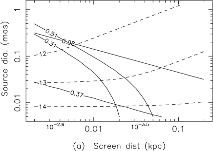
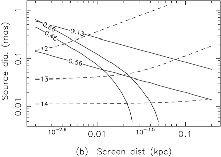
Figure 10: The trade-offs possible between scattering distance and angular diameter of the compact source. Solid contours are shown for the upper and lower observational limits on the scintillation time scale ($\tau_{I}$ in hours) and the scintillation index $m_{c}$ for the compact component. The dashed contours give the source brightness temperature (K) marked by the exponent of 10. (a) is for scattering from a screen at 8.6 GHz (b) is for a screen at 4.8 GHz. The distance axis is also annotated with the scattering measure as explained in the text.

The results are shown in Figure 10a as contours of $m_{c}$ and $\tau_{I}$ in the plane of $\log_{10}(L_{kpc})$, $\log_{10}(\theta_{\rm mas})$ calculated at 8.6 GHz for a screen. The observations constrain the values of $m_{c}$ and $\tau_{I}$, as described in Section 4.1. Hence the allowed scattering distance and source diameter are bounded by the two pairs of solid contours. Approximately, the screen distance is constrained by $2\mathbin{\lower 3.0pt\hbox{$\hbox to0.0pt{\raise 5.0pt\hbox{$\char 60\relax$}\hss}\mathchar 29208\relax$}}L\mathbin{\lower 3.0pt\hbox{$\hbox to0.0pt{\raise 5.0pt\hbox{$\char 60\relax$}\hss}\mathchar 29208\relax$}}50$ pc with associated source diameter $0.3\mathbin{\lower 3.0pt\hbox{$\hbox to0.0pt{\raise 5.0pt\hbox{$\char 62\relax$}\hss}\mathchar 29208\relax$}}\theta_{\rm mas}\mathbin{\lower 3.0pt\hbox{$\hbox to0.0pt{\raise 5.0pt\hbox{$\char 62\relax$}\hss}\mathchar 29208\relax$}}0.005$ mas. The peak brightness of the source can also be estimated for each point on the plane and is shown by the dashed contours, computed as follows. To find the brightness temperature we need the mean compact flux density $S_{c}$ and its angular diameter. The diameter is given at each point and $S_{c}$ can be estimated as $S_{rms}/m_{c}$ where $S_{rms}$ is the observed rms in flux density and $m_{c}$ is calculated for each point. Thus the diagram shows the allowed range in $\theta_{\rm mas}$, $L_{kpc}$ and $T_{b}$. Figure 10b shows a similar screen calculation based on the 4.8 GHz observations. The latter give the constraints $1\mathbin{\lower 3.0pt\hbox{$\hbox to0.0pt{\raise 5.0pt\hbox{$\char 60\relax$}\hss}\mathchar 29208\relax$}}L\mathbin{\lower 3.0pt\hbox{$\hbox to0.0pt{\raise 5.0pt\hbox{$\char 60\relax$}\hss}\mathchar 29208\relax$}}30$ pc with associated source diameter $0.6\mathbin{\lower 3.0pt\hbox{$\hbox to0.0pt{\raise 5.0pt\hbox{$\char 62\relax$}\hss}\mathchar 29208\relax$}}\theta_{\rm mas}\mathbin{\lower 3.0pt\hbox{$\hbox to0.0pt{\raise 5.0pt\hbox{$\char 62\relax$}\hss}\mathchar 29208\relax$}}0.04$ mas.

Though the limits on $L$ from the two frequencies clearly overlap, the two diameter limits at first appear to be less consistent. However, in comparing source diameters at 4.8 GHz with those at 8.6 GHz, we need to consider how the effective compact source diameter might depend on frequency. We first considered a uniform self-absorbed synchrotron source with diameter independent of frequency ($f$). However, the predicted frequency scaling for $S_{\rm rms}$ was then inconsistent with the observed $S_{\rm rms}\propto f^{-0.5}$.

We proceed by assuming that the core is limited by the same maximum brightness temperature at 4.8 and 8.6 GHz and that $S_{c}$ has a spectral index equal to 0.3, as observed for the avearge total flux density between these frequencies. This gives the effective diameter $\theta_{\rm mas}\propto f^{-1}\sqrt{S_{c}}\propto f^{-0.85}$. Accordingly, the angular diameter limits at 4.8 GHz are expected to be greater by a factor of 1.65 than at 8.6 GHz, though the factor is uncertain because of uncertainty in the fraction of flux density in the compact core. So in Figure 10b the 4.8 GHz angular diameter divided by 1.65 can be interpreted as the effective diameter at 8.6 GHz and compared with limits in Figure 10a. Thus dividing the 4.8 GHz diameter limits by 1.65 we find $0.36\mathbin{\lower 3.0pt\hbox{$\hbox to0.0pt{\raise 5.0pt\hbox{$\char 62\relax$}\hss}\mathchar 29208\relax$}}\theta_{8.6,\rm mas}\mathbin{\lower 3.0pt\hbox{$\hbox to0.0pt{\raise 5.0pt\hbox{$\char 62\relax$}\hss}\mathchar 29208\relax$}}0.025$ mas. The joint constraint on the diameter at 8.6 GHz is $0.36\mathbin{\lower 3.0pt\hbox{$\hbox to0.0pt{\raise 5.0pt\hbox{$\char 62\relax$}\hss}\mathchar 29208\relax$}}\theta_{8.6,\rm mas}\mathbin{\lower 3.0pt\hbox{$\hbox to0.0pt{\raise 5.0pt\hbox{$\char 62\relax$}\hss}\mathchar 29208\relax$}}0.025$ mas associated with $2\mathbin{\lower 3.0pt\hbox{$\hbox to0.0pt{\raise 5.0pt\hbox{$\char 60\relax$}\hss}\mathchar 29208\relax$}}L\mathbin{\lower 3.0pt\hbox{$\hbox to0.0pt{\raise 5.0pt\hbox{$\char 60\relax$}\hss}\mathchar 29208\relax$}}30$pc and $5\times 10^{11}\mathbin{\lower 3.0pt\hbox{$\hbox to0.0pt{\raise 5.0pt\hbox{$\char 60\relax$}\hss}\mathchar 29208\relax$}}T_{b}\mathbin{\lower 3.0pt\hbox{$\hbox to0.0pt{\raise 5.0pt\hbox{$\char 60\relax$}\hss}\mathchar 29208\relax$}}2\times 10^{13}$ K. Also noted on the horizontal axis of the diagram are values for the scattering measure of the screen ($SM$), which is the line-of-sight integral of $C_{N}^{2}$.

The allowed ranges of $L$ and $\theta_{\rm mas}$ also depend on several of the other assumptions in the model which we now discuss. Changing the axial ratio to 1.0 causes longer scintillation times and so shifts the time scale contours about a factor 1.4 toward even smaller distances; however, we have already argued that isotropic models are excluded, since they do not explain the negative overshoot in the acfs.

Another variable is the transition frequency $f_{w}$ between weak and strong scintillation, which we have taken to be 4.0 GHz. For a point source $m_{c}$ peaks near $f_{w}$. As the source size increases $m_{c}$ is reduced and its peak is shifted to frequencies below $f_{w}$, as can be seen from Figure 3 of R95. We observe a peak in $m_{c}$ near 4.8 GHz and so $f_{w}$ could possibly be above 4.8 GHz. Such a change would shift the $m_{c}$ contours upward in Figure 10, which further reduces both the scattering distance and the source brightness.

We also examined the effect of a Gaussian profile of scattering with the 1/e path length $L_{g}$. Since such a model includes some scattering very close to the Earth, this allows an increase in $L_{g}$ (compared to screen distance $L$), by a factor of about 1.5, allowing a smaller diameter (and brighter) source and a scattering path length up to 70 pc. However, given that the Gaussian profile does not fit the overshoot behavior in the auto-correlations, we now confine our attention to the screen models.

The velocity for the diffraction pattern is another important parameter, which we assume to be 36 km s^-1, the velocity of the Earth relative to the LSR. Increasing the velocity to 75 km s^-1 (the upper limit from Jauncey et al., 2000) changes the mapping from time scale to spatial scale, allowing a larger distance and smaller source size. The contours for time $\tau_{I}$ depend on $V$, $L$ and $\theta_{\rm mas}$ such that the upper limit for $L$ scales as $V_{\rm iss}^{2}$, while the lower limit scales linearly with $V_{\rm iss}$. The combined limits from plots as in Figure 10 recomputed for 75 km s^-1 give ranges $8\mathbin{\lower 3.0pt\hbox{$\hbox to0.0pt{\raise 5.0pt\hbox{$\char 60\relax$}\hss}\mathchar 29208\relax$}}L\mathbin{\lower 3.0pt\hbox{$\hbox to0.0pt{\raise 5.0pt\hbox{$\char 60\relax$}\hss}\mathchar 29208\relax$}}100$ pc associated with $0.13\mathbin{\lower 3.0pt\hbox{$\hbox to0.0pt{\raise 5.0pt\hbox{$\char 62\relax$}\hss}\mathchar 29208\relax$}}\theta_{8.6,\rm mas}\mathbin{\lower 3.0pt\hbox{$\hbox to0.0pt{\raise 5.0pt\hbox{$\char 62\relax$}\hss}\mathchar 29208\relax$}}0.013$ mas and $2\times 10^{12}\mathbin{\lower 3.0pt\hbox{$\hbox to0.0pt{\raise 5.0pt\hbox{$\char 60\relax$}\hss}\mathchar 29208\relax$}}T_{b}\mathbin{\lower 3.0pt\hbox{$\hbox to0.0pt{\raise 5.0pt\hbox{$\char 60\relax$}\hss}\mathchar 29208\relax$}}6\times 10^{13}$ K.

The conclusion from the foregoing, rather lengthy discussion is that for our preferred model (with $f_{w}\sim 4$ GHz) the modulation index and time scale for IDV of PKS 0405-385 at 4.8 and 8.6 GHz require a very local scattering region, in a screen in the range 2 to 30 pc. The overshoot in the acfs, which require substantially anisotropic scattering (axial ratio $\mathbin{\lower 3.0pt\hbox{$\hbox to0.0pt{\raise 5.0pt\hbox{$\char 60\relax$}\hss}\mathchar 29208\relax$}}0.25$). We presume that the orientation of the anisotropic structure in the plasma is determined by the local mean magnetic field and that a pronounced anisotropy implies a uniform field through the scattering plasma. This is more reasonable physically if the scattering is localized in a thin layer (screen) rather than in an extended scattering medium, in which the magnetic field would tend to be disorganized.

Associated with the distance and velocity limits there are allowed ranges of maximum source brightness in the range $5\times 10^{11}$K to $\sim 6\times 10^{13}$K for the nominal screen model. Our nominal brightness limits are about 25 times lower than inferred by KCJ, who based their analysis on the greater scattering distances of the TC93 model for the IISM. We also note that there is an inverse relation of brightness and the fraction of the total flux density in the compact core (100% for the lowest brightness down to about 25% for the highest brightness).

5 ISS of the Stokes Parameters

In several IDV sources the fluctuations in $I$ are accompanied by fluctuations in the linear polarization parameters $Q$ and $U$. Figures 1 – 4 , 6 & 7 show that, for PKS 0405-385 the polarization parameters vary faster than does $I$, as is often the case for other IDV sources (Q89, Gabuzda, 2000a,b,c). As discussed below, in the ISS of a linearly polarized point-source $Q(t)$ and $U(t)$ should simply be scaled versions of the variations in $I(t)$. Figures 1, 2, 3 and 4 show that the Stokes’ variations in PKS 0405-385 are clearly inconsistent with such behaviour.

As will be shown below, when the polarization structure differs from that of the total flux density, the $Q$ and $U$ scintillations become partially decorrelated from those in $I$. We now develop the appropriate theory and in section 6 we search for a particular polarized source structure that matches the observations of PKS 0405-385. Though observers often display fluctuations in polarized flux density $P=\sqrt{Q^{2}+U^{2}}$ (or polarized degree $p=P/I$) and position angle $\chi=0.5\tan^{-1}(U/Q)$, we choose $Q,U$, since they sum linearly from incoherent regions of emission.

We analyze ISS from a source whose structure in $Q$ and $U$ may differ from that in $I$. An entirely parallel formulation can be done for $V$, though it is not considered in this paper. A brief outline of these results was given by Rickett (2000) and an entirely similar analysis was used by Medvedev (2000) in the context of strong scintillations, applied to the radio afterglows of gamma ray bursts. In Section 3 we quantified the relationship between fluctuations in $I$,$Q$ and $U$ by their six auto- and cross-correlation functions. Thus we develop the theory for these correlations, assuming weak or refractive ISS. The method is simply a repeated application of the smoothing formula as expressed by Little and Hewish (1966) and Salpeter (1967).

Consider a scattering layer (screen) of thickness $\delta z$ at distance $z$ from an observer who receives polarized waves from a source whose brightness distribution in $I$ is $B_{I}(\theta_{x},\theta_{y})$. Let $\Delta I_{o}(x,y)$ be the pattern of intensity fluctuation about its mean for a unit flux density point source located on the z-axis at a great distance. The net flux density is the sum of shifted terms weighted by each brightness element:

$$\Delta I(x,y)=\int\int\Delta I_{o}(x-z\theta_{x},y-z\theta_{y})B_{I}(\theta_{x},\theta_{y})d\theta_{x}d\theta_{y}\;,$$ (10)

where infinite limits are implied in this and subsequent integrals since the brightness functions are confined to small angles. Exactly similar equations can be written for $\Delta Q$ and $\Delta U$ for a source with polarized brightness functions $B_{Q}(\theta_{x},\theta_{y})$ and $B_{U}(\theta_{x},\theta_{y})$, since the ISS in, say, $Q$ due to each source element is simply $\Delta I_{o}(x-z\theta_{x},y-z\theta_{y})B_{Q}(\theta_{x},\theta_{y})d\theta_{x}d\theta_{y}$.

The important underlying assumption here is that the scintillation conditions in the right and left circular modes of propagation through the magneto-ionic plasma are essentially identical. For radio-astronomical signals travelling through the ISM the phase difference in the two modes is twice the angle of Faraday rotation on that line of sight. From the mean polarization angle observed versus wavelength we estimate a rotation measure $RM\sim 70$ rad m^-2, which at 8.6 GHz gives $\mathbin{\lower 3.0pt\hbox{$\hbox to0.0pt{\raise 5.0pt\hbox{$\char 60\relax$}\hss}\mathchar 29208\relax$}}0.2$ radian phase difference between left and right. This is very small compared to the total phase increment due to the plasma, for which a typical value might be $10^{7}$ radians ($\propto\lambda$). To put it more precisely, any scintillation in $p$ or $\chi$ for a point source will be negligible, if across a Fresnel scale there is a negligible change in this right-left phase difference. Observational evidence for this condition in the typical ISM is obtained from Haverkorn et al. (2000), who used the Westerbork telescope to observe the polarized Galactic background. They observed about 1 radian changes in its polarization angle over a scale as small a 4 arc-minutes near a Galactic latitude of 16 degrees at a wavelength of 1.1 meter. At an assumed distance of 500 pc for the magneto-ionic medium, this corresponds to about 0.5 pc and maps at 8.6 GHz to a typical change in the Faraday phase on scale $r_{F}$ of about $10^{-8}$ radians . This confirms that there should be negligible point-source scintillation in the degree or angle of polarization.

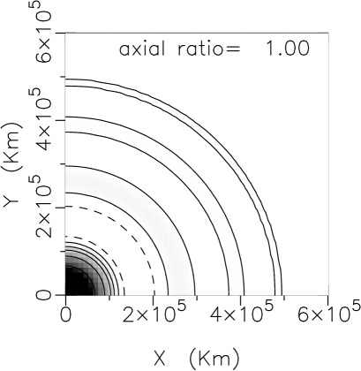
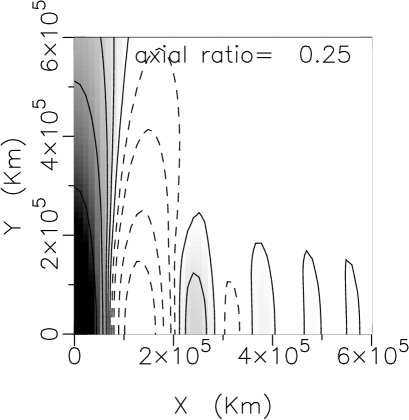
Figure 11: Contour plots of $C_{oo}(\vec{\sigma})$ in a single quadrant (function is symmetric about both axes). Axial ratio 1.0 in left panel and 0.25 in right panel. The dashed contours are negative at (-0.05, -0.1, -0.2, -0.3) only for only for the latter are there deep negative lobes; the shaded solid contours visible are at (0.4, 0.2, 0.1, 0.05, 0.0). Here $r_{F}=6.7\times 10^{4}$km.

For a very distant point source the ISS variations due to a screen are approximately statistically homogeneous, thus the spatial auto-correlation for $\Delta I_{o}$ depends only on the spatial separation $(\xi,\eta$), not on absolute position:

$$C_{oo}(\xi,\eta)=<\Delta I_{o}(x,y)\Delta I_{o}(x+\xi,y+\eta)>$$ (11)

Similar correlations versus spatial offsets can be defined for each pair of observed Stokes’ parameters in a fashion analogous to equations (3), for example:

$$C_{IQ}(\xi,\eta)=<\Delta I(x,y)\Delta Q(x+\xi,y+\eta)>$$ (12)

Substituting equation (10) and the parallel equation for $\Delta Q$ into (12), one finds:

$$C_{IQ}(\xi,\eta)=\int\int C_{oo}(\xi-z\alpha_{x},\eta-z\alpha_{y})R_{IQ}(\alpha_{x},\alpha_{y})d\alpha_{x}d\alpha_{y}\;,$$ (13)

where

$$R_{IQ}(\alpha_{x},\alpha_{y})=\int\int B_{I}(\beta_{x}-\alpha_{x}/2,\beta_{y}-\alpha_{y}/2)B_{Q}(\beta_{x}+\alpha_{x}/2,\beta_{y}+\alpha_{y}/2)d\beta_{x}d\beta_{y}\;.$$ (14)

There are also similar results for the other auto- and cross-correlations ($II$, $QQ$, $UU$, $IU$, $QU$). Each gives the observed correlation function as a convolution of the cross-correlation of the two brightness distributions by an ISS resolution function $C_{oo}(\xi,\eta)$, which is plotted in Figure 11 for axial ratios 1.0 and 0.25.

As mentioned in Section 4 we are concerned with refractive ISS in strong scintillation or with weak ISS. In both cases the convolution results apply and so theoretical expressions for $C_{oo}(\xi,\eta)$ are given by products in the wavenumber domain. Thus each spectrum is the product of the point source scintillation power spectrum by a source filter, which is the Fourier transform of the source brightness correlations $R_{II}$, $R_{IQ}$ etc. For $R_{II}$ the source filter is the squared magnitude of the visibility function as already given explicitly in equation 9. This is the so-called “Cohen-Salpeter” equation (Salpeter, 1967). For the cross-spectrum between $I$ and $Q$ the filter becomes complex (e.g. $V_{I}V_{Q}^{*}$), giving:

$$P_{IQ}(\kappa_{x},\kappa_{y})=8\pi r_{e}^{2}\lambda^{2}C_{N}^{2}\delta z\;(R\kappa_{x}^{2}+\kappa_{y}^{2}/R)^{-\alpha-2}\sin^{2}(z\kappa^{2}\lambda/4\pi)\times$$

$$V_{I}(\kappa_{x}z/2\pi,\kappa_{y}z/2\pi)V_{Q}^{*}(\kappa_{x}z/2\pi,\kappa_{y}z/2\pi)$$ (15)

Note that the x-direction is defined here by the orientation of the ellipse in wavenumber, such that for $R<1$ the minor axis of the spatial correlation ellipse lies along the x-axis; this defines the coordinate frame for our fitted source models. Equations (15 and 9) apply to weak scintillation and to refractive scintillation in which the source filter cuts-off the scintillations at a lower wavenumber than the refractive cut-off (at the inverse of the scattering disc size). Such conditions seem to apply for most extragalactic sources observed away from the Galactic plane.

We compare theory with the observations in the time domain and so we compute the model as a two-dimensional Fourier transform of each wavenumber spectrum – for example:

$$C_{IQ}(\xi,\eta)=\int\int P_{IQ}(\kappa_{x},\kappa_{y})\exp[i(\kappa_{x}\xi+\kappa_{y}\eta)]d\kappa_{x}d\kappa_{y}.$$ (16)

We then map spatial lags to temporal lags for a given model velocity.

The other geometry to be considered is a scattering medium that extends from the observer out through the Galactic disc. We have chosen to model this by the Gaussian in equation (8) with scale length $L_{g}$. Putting this into equation (15) and integrating over $z$ from zero to infinity gives expressions for the auto- and cross spectra, which can be integrated analytically for Gaussian brightness functions. Details are shown in Appendix B. The Gaussian functions give explicit equations that allow efficient computation. It is unlikely that different functional forms for the tapering of the tail of profile will make much difference to the calculations. Many other geometries can be considered between the extremes of a screen and a Gaussian profile. Coles (1988) shows that, when the scattering medium does not continue up to the observer for even a small fraction of $L_{g}$, the shape of the acf starts to approximate the screen result.

6 Model-Fitting the Stokes’ Correlations at 8.6 GHz

We note that it is not possible in general to construct model time series for $Q(t)$ and $U(t)$ from $I(t)$ for more than one source component, since the ISS creates a two dimensional stochastic pattern, of which the observations only sample a one-dimensional slice. Consequently, we compare the 8.6 GHz Stokes’ correlations with computed models using the theory of the previous section. We initially considered an algorithm like CLEAN, as used in image synthesis in which a model for the visibility function is built by adding a sequence of Gaussian components. However, this is not feasible here, since the Stokes’ correlations depend on the square of the visibility (equation 15). The associated cross-products between every pair of components makes the addition of components non-linear. Thus we used conventional least-squares minimization on the model correlation functions.

The models require specification of both the scattering medium and the polarized source structure, with parameters summarized in Table 3. The important parameters of the scattering medium have already been discussed. In our fitting we fixed $L=25$ pc, $\alpha=5/3$, at the Kolmogorov value. We also fixed the axial ratio $R$ to be 0.25 and the velocity of Earth relative to the scattering plasma $V_{iss}$ as described in section 4.1; though its orientation relative to the minor axis of the scattering irregularities was a fitted parameter.

We model the source structure as the superposition of circular uniformly polarized Gaussian components. Each is characterized by its flux density, its fractional linear polarization and position angle, its FWHM diameter and its angular position relative to a central component, again referred to the minor axis of the scattering irregularities. The number of parameters to model the source increases from 4 for a single source to 10 for two components to 16 for three components. We now describe attempts to model the data with one, two and three components.

We first considered a single Gaussian component of uniform polarized fraction $p_{1}$ and position angle $\chi_{1}$. In this case the brightness distributions of $Q$ and $U$ are exactly proportional to the brightness distribution in $I$, and so the polarized ISS will be like that for a polarized point source, in that the fluctuations $Q(t)$ and $U(t)$ should be simple linearly scaled versions of $\Delta I(t)=I(t)-<I>$. This model requires four constant coefficients, which we estimated from a least-squares fit to the observed $Q(t)$ and $U(t)$, as shown by the solid lines in Figure 1. These are clearly unsatisfactory. Expressed another way, the six Stokes’ correlation functions of Figure 6a would all follow the form of the acf, except that the ccfs could be sign inverted depending on the signs of $Q$ and $U$. This is also clearly incompatible with the observations. We conclude that a single component of uniform polarized fraction and position angle does not explain the polarized IDV. We note that this analysis and conclusion apply in the presence of an added non-scintillating component with a different linear polarization, even though in such a case the overall polarized fraction and angle may become time variable.

6.1 Multi-Component Models

Moving to multi-component source models, we use a non-linear least-squares optimization scheme to search for source parameters to best fit the six Stokes’ correlations. In Figure 6 we plotted the correlations averaged over the three full 12-hour tracks of the source (June 8, 9, 10) at both 4.8 and 8.6 GHz. It is difficult to estimate the statistical errors associated with these functions, and so we also computed the correlations for each of the individual days. Here it was clear that the main features of the 8.6 GHz correlations were recognizable in both auto- and cross- correlations for each of the individual days; however, at 4.8 GHz the features in the cross-correlations were much less repeatable. Consequently, we concentrate on model-fitting to the 8.6 GHz observations, since they show the most consistent behaviour in the correlation functions.

The theoretical expressions for the temporal correlations are obtained from the spatial correlation functions by mapping spatial lags to temporal lag ($\tau$) according the the velocity model ($V_{iss,x},V_{iss,y}$).

$$C_{IQ,t}(\tau)=C_{IQ}(\xi=V_{iss,x}\tau,\eta=V_{iss,y}\tau).$$ (17)

Here $C_{IQ}(\xi,\eta)$ is given by the Fourier transform (16) of the spectrum from equation (15). Thus for a given set of model parameters we compute the six correlations $C_{II,t}$, $C_{QQ,t}$, $C_{UU,t}$, $C_{IQ,t}$, $C_{IU,t}$, $C_{QU,t}$ at the time lags observed. We minimize the following function, which is the weighted sum of the squared differences (observation - theory) from all six correlation functions:

$$S^{2}=\Sigma^{i,q,j}wt(\tau_{j})[C_{iq,t,obs}(\tau_{j})-C_{iq,t,theory}(\tau_{j})]^{2}/\sigma_{iq,j}^{2}/\Sigma^{i,q,j}wt(\tau_{j})$$ (18)

where $i$ and $q$ are each $I,Q$ or $U$, $\sigma_{iq,j}$ is the rms error in the correlations and $wt(\tau_{j})$ is a triangular weight falling to zero at times of $\pm 3$ hrs. We choose these limits on time lag since it is known that errors in correlation estimates remain high at large lags, whereas the signal is expected to decrease. Therefore we do not consider source models in which there could be components separated by angles substantially greater than their diameters, since in that case correlations could extend to large time lags.

Figure 12: Auto- and cross-correlations at 8.6 GHz as in Figure 6, overplotted with a best fit model with 2 scintillating source components and scattering localized in a screen.

With two scintillating source components, there are 15 parameters, of which 4 were fixed at the values given in Table 3. In searching the remaining 11 parameters we find a satisfactory fit to five of the six correlation functions, as shown in Figure 12. However, the model fails to reproduce the offset peak visible at a time lag of 0.3 hrs in $C_{QU,t}(\tau)$. Further it does not fit the $Q-Q$ and $U-U$ correlations very well. The minimum value of the reduced chi-squared error ($S^{2}$) is 5.6, significantly worse than 1.0 expected for a satisfactory fit. If we exclude $C_{QU,t}(\tau)$ a better fit can be obtained to the remaining five correlations with a (satisfactory) minimum $S^{2}\sim 1.4$. Figure 13 shows the source brightness distribution for the fit of Figure 12. The brightness plots were calibrated in Kelvin by the following procedure.

Figure 13: Brightness distributions for the two component source model used in Figure 12. The angular scale is in mas, with the horizontal axis parallel to the minor axis of the ISM anisotropy ellipse (whose absolute orientation is not known). The relative direction of velocity vector is shown by the arrow. The left panel shows the total brightness temperature with the peak at $\sim 10^{14}$K. The right panel shows contours of polarized brightness $P$ with a maximum of 53% of the total with bars showing $P$ and position angle $\chi$. The contour levels decrease logarithmically (5 levels per decade)

The scaling of the brightness contours depends on the total compact flux density ($S_{c}$), which is not estimated during the model fitting, since the auto- and cross-correlations are normalized. However, $S_{c}$ can be estimated from $S_{rms}/m$, where $m$ is the scintillation index from the model. In addition to the other parameters, this requires an estimate of the scattering measure (SM), which we determined from our constraint on the transition frequency $3.0\mathbin{\lower 3.0pt\hbox{$\hbox to0.0pt{\raise 5.0pt\hbox{$\char 60\relax$}\hss}\mathchar 29208\relax$}}f_{w}\mathbin{\lower 3.0pt\hbox{$\hbox to0.0pt{\raise 5.0pt\hbox{$\char 60\relax$}\hss}\mathchar 29208\relax$}}4.8$ GHz, as already discussed; the corresponding uncertainty in the maximum derived brightness is about a factor two.

The brightness has a maximum of close to $10^{14}$K at the origin of the plot and the degree of polarization is a maximum of 43%. These interesting physical estimates will be discussed in the next section after presentation of three-component models. The basic topology that fits the polarization behaviour is a pair of components with approximately orthogonal linear polarization, separated by about 10 $\mu$as along the ISS velocity direction, which is inclined at about 30 degrees to the minor axis of the scattering irregularities. The components must also be displaced by some distance perpendicular to the velocity since the maximum $QU$ cross correlation is not 100%; a perpendicular separation of 5-10 $\mu$as ensures that the scintillation from the two components are only partially correlated. Since we were unable to find a two component model that matches all six correlations and we believe that the offset in the peak in $C_{QU,t}(\tau)$ is significant, we tried three components.

With three scintillating source components, there are 21 parameters, of which 4 were fixed as given in Table 3. In searching the 17 variable parameters we find good fits to all six correlation functions. However, the optimum is not uniquely determined – there is a set of satisfactory solutions, with minimum $S^{2}$ of about 1.4. Since there is still substantial uncertainty about the correct normalization of the errors in the auto- and cross-correlations, there is a corresponding uncertainty about the absolute normalization in $S^{2}$. Consequently, we accept 1.4 as a satisfactory fit and do not attempt a more complex model, which would require even more parameters. The example shown in Figure 14 is one which minimizes the peak brightness temperature. The brightness distribution in total flux density and in polarized flux density are shown in Figure 15, in which the maximum total brightness temperature is $\sim 2\times 10^{13}$K and the peak polarization degree of $\sim 70$%. Note that the model uses three components of uniform polarization degree and angle, with the central component extending over $\sim 30\mu$as. Since its polarization is nearly orthogonal to that of the other two smaller components, the net polarization has a minimum near the center, creating four regions of polarized brightness.

There are in fact many other source models with higher peak brightness (but no significant improvement in the fit), but there are no satisfactory fits with significantly lower brightness temperatures than in the fit displayed. Thus though the model shown here is by no means unique, it clearly demonstrates that a source model can be found to give a quantitative fit to the correlations among the Stokes’ parameters with a physically reasonable degree of polarization and with a maximum brightness $\sim 2\times 10^{13}$K. While this is high it is consistent with Doppler beaming factors implied from VLBI measurements of apparently superluminal motion in other AGNs.

Figure 14: Auto- and cross-correlations at 8.6 GHz as in Figure 6, overplotted with a fit to a 3-component model. This fit minimizes the peak brightness temperature among the other similar models

Figure 15: Brightness distributions for the three component source model used in Figure 14. The angular scale is in mas plotted in the format of Figure 13. The left panel is the total brightness temperature with the peak at about $2\times 10^{13}$K. The right panel is the polarized brightness with maximum $\sim 70$% of the total brightness.

Symbol	Parameter	2-comp	3-comp
$L$	screen distance (pc)	25*	25*
$R$	axial ratio	0.25*	0.25*
$V_{iss}$	ISS velocity (km s-1)	36*	36*
$\psi$	direction of ISS velocity	$28^{\circ}$	$11^{\circ}$
$\alpha$	spectral exponent	5/3*	5/3*
$S_{I,1}$	Total flux density (Jy)	0.38	0.48
$\theta_{1}$	FWHM ($\mu$as)	15	30
$P_{1}$	polarized flux density (Jy)	0.18	0.33
$\chi_{1}$	polarized PA	$23^{\circ}$	$-29^{\circ}$
$S_{I,2}$	Total flux density comp 2 (Jy)	0.19	0.024
$\theta_{2}$	FWHM ($\mu$as)	9.4	19
$P_{2}$	polarized flux density comp 2 (Jy)	0.17	0.22
$\chi_{2}$	polarized PA	$-65^{\circ}$	$63^{\circ}$
$\theta_{ox,2}$	comp 2 position ($\mu$as)	-1.9	-4.
$\theta_{oy,2}$	comp 2 position ($\mu$as)	-6	1.6
$S_{I,3}$	Total flux density (Jy)	0	0.091
$\theta_{3}$	FWHM ($\mu$as)	-	$19\mu$as
$P_{3}$	polarized flux density comp 2 (Jy)	-	0.11
$\chi_{3}$	polarized PA	-	$56^{\circ}$
$\theta_{ox,3}$	comp 3 position ($\mu$as)	-	11
$\theta_{oy,3}$	comp 3 position ($\mu$as)	-	-2

Table 3: Model parameters. The values with an asterisk were fixed in the fits. Angles are given relative to the minor axis of the scattering ellipse (defined in equation 15). Polarized position angles are defined as for the observations. Though the polarized flux densities for components 2 and 3 are greater than 70% of their individual total flux densities, the polarized brightness is everywhere less than 70% of the total brightness in these models, as displayed in Figures 13 and 15. See text concerning the lack of uniqueness in the parameters.

The fits displayed and discussed above are all based on a screen model for the scattering medium. As discussed in section 4.2 the effect of a Gaussian profile of scattering was also computed and shown to reduce the amplitude of the overshoot in the auto-correlations. While the screen model gives less overshoot than observed, it does agree within about $1\sigma$. The Gaussian profile models gave less overshoot and disagree by $\mathbin{\lower 3.0pt\hbox{$\hbox to0.0pt{\raise 5.0pt\hbox{$\char 62\relax$}\hss}\mathchar 29208\relax$}}2\sigma$. In view of this systematically worse fit, we did not attempt source model fits for the Gaussian profile.

6.2 Stokes’ Correlations at 4.8 2.4 and 1.3 GHz

The Stokes’ parameters at the three lower frequencies have generally lower amplitudes than at 8.6 GHz (Table 1) and their correlations have greater statistical errors. Consequently, we did not attempt detailed model fits to their Stokes’ correlation functions. Nevertheless, the lower frequency results are part of the IDV data to be explained. There are two relevant effects. The first is the possible suppression of ISS in the local screen by angular broadening in the “normal” Galactic plasma scattering. The second is increasing Faraday rotation and depolarization in the source itself. We suggest that a combination of these effects explains the lower amplitude IDV in $Q$ and $U$ and the lack of systematic correlation with the IDV in $I$.

The TC93 model predicts a path length through the IISM of about 1000 pc toward PKS 0405-385, at a Galactic latitude of -48 degrees. The model is a smooth representation of the dispersing and scattering observed for pulsars, which is known to be quite “patchy”. However, it would be surprising if on our line of sight there were no more distant scattering electrons than at 25-100 pc. The scattering measure ($SM$) on that line of sight, found by integrating the TC93 model for $C_{N}^{2}$, is $SM=2.0\times 10^{-4}$ m^-20/3 kpc, which is comparable to the values for the scattering model used in our model and in Figure 10.

This must cause an angular broadening, which may be sufficient to suppress the scintillation in the local region. The angular scattering diameter (FWHM), which depends on $SM$ and the frequency (see Cordes et al., 1991, for example), is 7 $\mu$as at 8.6 GHz and 24 $\mu$as at 4.8 GHz. This will be most critical in the ISS of the smallest structures in our 8.6 GHz model. which are low flux density highly polarized components with diameters $\sim 20\mu$as. If at 4.8 GHz these were scatter broadened to 24 $\mu$as the rms amplitude of their fluctuations would be significantly decreased over those at 8.6 GHz, while at the same time the rms amplitude in $I$ at 4.8 GHz will increase, since 4.8 GHz is above $f_{w}$.

Further reduction in $Q_{\rm rms}$ and $U_{\rm rms}$ will result from increasing depolarization within the source below 8.6 GHz. As is widely observed, internal Faraday depolarization increases strongly with decreasing frequency. The mean degree of polarization in PKS 0405-385 decreases below 8.6 GHz, and so too must the peak level of polarized brightness, which will reduce the amplitude of polarized ISS.

We interpret the 2.4 and 1.4 GHz IDV as refractive ISS at frequencies below $f_{w}$, since the time scales are substantially larger than at the two higher frequencies. In trying to compare these longer time scales with theory, we could compute the expected time scales for refractive ISS, following the R95 method. However, this method does not include the diffractive ISS contributions at frequencies just below $f_{w}$ and so overestimates the time scale and underestimates the modulation index for a source as compact as PKS 0405-385. Simulation techniques are needed to model the scattering at these frequencies.

In a separate investigation at 1.4 GHz, we considered the possibility that Faraday depolarization across the receiver bandpass could have reduced the peak polarization and so reduced the amplitude of ISS in $Q$ and $U$. We looked separately in the 8 sub-bands for $Q,U$ fluctuations and found no significant differences. Thus there is no evidence for more compact polarized components at 1.4 GHz, which might show more rapid (diffractive) ISS in polarization. This is consistent with the suggestion above that at the lower frequencies the fine structure in polarized brightness is suppressed by depolarization in or near the source.

6.3 Discussion of the Fits

Whereas two source components are adequate to model five of the six Stokes’ correlations, a third component is necessary to adequately model the $QU$ correlation. Thus the observed form of $C_{QU,t}(\tau)$ has a strong influence on the best fitting 3-component source model. In particular figure 14 shows peaks at lags of -2.0, -0.4 and 0.3 hrs and accompanying minima at -1.1, -0.2 and 0.8 hrs. The model shown matches well from -1 to 0.7 hrs, but fails to follow the peaks and valleys further out. On close inspection we also see that the negative overshoot in $C_{QQ,t}(\tau)$ and $C_{UU,t}(\tau)$ is also not well modelled.

The model shown has the least rms residual near one local minimum of the parameter space. There are nearby regions in which the residual changes little and the peak brightness increases. However, we did not search exhaustively for other local minima far removed from this one. In particular we did not explore models with component separations larger than about 0.04 mas, which when mapped into time by $\tau=L\theta/V$ corresponds to about 1.3 hrs. Thus our model does not include a source sufficiently extended that could generate peaks at lags of 2-3 hrs from the origin, such as those visible in several of the correlations. Looking at the correlations over time lags out to $\pm 7$ hrs in Figure 6, one sees that the large amplitude correlations do extend out to at least 3 hrs. While we chose to parameterize three circular components by their flux density, FWHM diameter, relative position, polarized flux density and position angle, it is possible that two elliptical components with gradients in position angle might also give satisfactory or better fits.

This discussion is relevant also to the lower level of the polarized ISS at the three lower frequencies (section 6.2). The ISS “resolution function” can be considered to be the function $C_{oo}(\xi,\eta)$ (in Figure 11) mapped into angular coordinates by dividing the spatial offsets by the scattering distance $L$. This function is elongated having a width equal to the Fresnel angle ($(Lk)^{-0.5}$) in $\theta_{x}$ and a factor four greater in $\theta_{y}$ for our assumed axial ratio. If at the lower frequencies there were polarized structures in which $Q$ or $U$ reversed sign on angles much smaller than the Fresnel angle, they would tend to average out to give little observable ISS in $Q$ or $U$ – that is they would be below the ISS resolution limit. We suggest that at the lower frequencies any polarized structures are subject to greater effects of internal Faraday rotation and depolarization, making complex polarization structure on scales finer than the Fresnel angle and so suppressing the polarized ISS. It is interesting that such a resolution limit does not apply for the ISS of total intensity since it cannot change sign. An assembly of sources finer than the Fresnel angle will still show ISS similar to that of a point source.

7 Discussion and Conclusions

Coupling of the Scattering and Source Models

In Section 4.3 we analyzed weak ISS at 4.8 and 8.6 GHz, caused in a localized layer of scattering at distance $L$ from the Earth, for a single Gaussian source component. A range $2\mathbin{\lower 3.0pt\hbox{$\hbox to0.0pt{\raise 5.0pt\hbox{$\char 60\relax$}\hss}\mathchar 29208\relax$}}L\mathbin{\lower 3.0pt\hbox{$\hbox to0.0pt{\raise 5.0pt\hbox{$\char 60\relax$}\hss}\mathchar 29208\relax$}}30$ pc matches the observations, with an associated range of source diameters $\theta_{\rm mas}$ (and a generally inverse relationship between these two parameters). A major finding of the paper is a reduction in the peak source brightness temperature to $\sim 2\times 10^{13}$ K, which is a factor 25 less than inferred in the earlier analysis of KCJ. This brings the relativistic bulk Doppler factor for the presumed jet closer to the inferred values from the superluminal motion of VLBI sources. While we assumed that the IISM velocity was that of the LSR (36 km s^-1 relative to the Earth in June), a velocity of 75 km s^-1, which is the upper bound from the intercontinental time delay in the ISS, changes the allowed ranges to $8\mathbin{\lower 3.0pt\hbox{$\hbox to0.0pt{\raise 5.0pt\hbox{$\char 60\relax$}\hss}\mathchar 29208\relax$}}L\mathbin{\lower 3.0pt\hbox{$\hbox to0.0pt{\raise 5.0pt\hbox{$\char 60\relax$}\hss}\mathchar 29208\relax$}}100$ pc, and $0.13\mathbin{\lower 3.0pt\hbox{$\hbox to0.0pt{\raise 5.0pt\hbox{$\char 62\relax$}\hss}\mathchar 29208\relax$}}\theta_{8.6,\rm mas}\mathbin{\lower 3.0pt\hbox{$\hbox to0.0pt{\raise 5.0pt\hbox{$\char 62\relax$}\hss}\mathchar 29208\relax$}}0.013$ mas and $2\times 10^{12}\mathbin{\lower 3.0pt\hbox{$\hbox to0.0pt{\raise 5.0pt\hbox{$\char 60\relax$}\hss}\mathchar 29208\relax$}}T_{b}\mathbin{\lower 3.0pt\hbox{$\hbox to0.0pt{\raise 5.0pt\hbox{$\char 60\relax$}\hss}\mathchar 29208\relax$}}6\times 10^{13}$ K, which is still a factor 8 smaller than inferred by KCJ.

Degree of Polarization

The observations provide values for $Q_{\rm rms}$ and $U_{\rm rms}$, but these were not included in the fitting, initially, since the normalized correlation functions are unaffected by the overall degree of polarization. This was remedied by adding two data points to the computation of the fitting residual $S^{2}$. The squared difference between model and observation of $Q_{\rm rms}$ and $U_{\rm rms}$ was added to $S^{2}$, with a weight such that each would be approximately equivalent to one of the auto-correlations. When included in the fit process, this reduced the peak brightness in the best fitting source models, and raised the maximum degree of polarization.

In the final two and three component models of Figures 13 and 15 the peak polarization degree is about 70%, which is close to the theoretical maximum from a uniform synchrotron source (see Gardner and Whiteoak 1966). However, this is not a coincidence, rather it is a result of an upper bound being placed on the maximum degree of linear polarization during the fitting process. The degree of polarization might also be affected by the addition of a polarized component, which is too extended to scintillate; depending on its position angle this would either increase or decrease the maximum degree of polarization. However, our model has about 1.3 Jy in a structure that is larger than $\mathbin{\lower 3.0pt\hbox{$\hbox to0.0pt{\raise 5.0pt\hbox{$\char 62\relax$}\hss}\mathchar 29208\relax$}}0.2$ mas, for which the peak brightness is too small to change the polarized brightness significantly. The model shown in Figure 14 has structure in $Q$ and $U$ on significantly finer scales than in $I$. Our model is the sum of three circular Gaussian components, creating a somewhat elongated structure. The polarized flux density of each component was constrained to be less than 70% of the total flux density of component 1. Though this allows weak Gaussian components with individual degrees of polarization greater than 100% (see Table 3), it keeps the polarization brightness less than 70 % of the total brightness at all points across the source, consistent with synchrotron theory. With this constraint the two-component model gave close agreement in $Q_{\rm rms}$ and $U_{\rm rms}$, while for the three-component model these quantities were about 25% below the observed values.

VLBI Observations and Time Evolution of the ISS

VLB observations of PKS 0405-385 were made in June 1996, revealing two components, barely resolved at 1 mas resolution (Kedziora-Chudczer et al., 2001). The flux density at 8.4 GHz in the “core” was 1.5 Jy with 0.24 Jy in a NW extension. We can ask how such a model might be reconciled with the episode of fast IDV in June 1996. Our results suggest that the IDV was due to 30 by 22 $\mu$as compact structure of about 0.5 Jy at 8.6 GHz and with $\sim 1.3$ Jy in a more extended component (jet?), part of which was picked up as a NW extension in the VLB image. From the observed IDV the compact core has a brightness temperature of $\sim 2\times 10^{13}$K, which we interpret as $\sim 3\times 10^{11}$K Doppler boosted in a relativistic jet. This implies a minimum Doppler factor of about 14, including the $1+z$ factor ($z=1.285$) in Marscher’s (1998) expression. Depending on the angle of the jet to the line of sight this corresponds to an apparent superluminal expansion of about 0.13 mas in two months. Thus the ultra compact feature causing the ISS may have expanded from 0.03 mas to 0.13 mas, which could have quenched the ISS substantially on the time scale of two months. Such behaviour differs considerably from the long-lived scintillation seen in the other two very rapid scintillating sources, J1819-4835 (DTB, Bignall et al., 2002)

Subsequently the total flux density of the source almost doubled over 1.5 years indicating further expansion of the previously scintillating component. In a separate paper we model this long term time evolution of the PKS 0405-385 as expanding compact knots in a more extended jet. However, we cannot yet rule out the alternative hypothesis that the changes in IDV are due to changes in the scattering in the local ISM.

The Local ISM

By greatly reducing the scattering distance, we have greatly reduced the source brightness temperature over that inferred by KCJ. Having replaced a source puzzle by an interstellar puzzle, we now consider the implications for the local interstellar medium (ISM) and look for any corroborating evidence on the line of sight toward the quasar ($l=119^{\circ},b=-48^{\circ}$).

The $SM$ values in the local ISM responsible for the IDV in PKS 0405-385 are $\sim 3\times 10^{-4}$ m^-20/3 kpc. This is comparable to value in the TC93 Galactic disk, which extends more than 10 times further than our screen distance. With a screen thickness of say 5 pc the local value of the scattering strength parameter ($C_{N0}^{2}$) must be about 100 times greater than in the TC93 model. This suggests we have detected a remarkable nearby concentration of very irregular plasma.

We compare this with the enhanced scattering at the edge of the “local bubble” (Bhat et al. 1998). They model their pulsar observations by an ellipsoidal shell with $SM=6\pm 3\times 10^{-5}$ m^-20/3 kpc, at 134 pc in the direction toward PKS 0405-385 (including the factor 3 reduction according to appendix C of Rickett et al., 2000). In the set of pulsars that they observed the closest was 45^∘ from our line-of-sight. Thus taking our observations and theirs together requires a much less regular structure than their ellipsoidal model of uniform $SM$, such that the scattering layer toward PKS 0405-385 has a 5 times greater $SM$ and lies at only 25-100 pc from the Earth. In an approximately orthogonal direction Rickett et al. (2000) deduced a deficit in scattering on the 310 pc line toward PSR B0809+74 and suggested patchiness in the shell of enhanced scattering. We can only conclude that the local IISM is spatially inhomogeneous in its turbulence, and we now consider other evidence on the local ISM toward PKS 0405-385.

The diffuse ionized component of the ISM mapped in the Southern H_α Sky Survey (Gaustad et al. 2001) does not reveal any distinct ionized region in this direction. The possibility of a turbulent stellar wind from a nearby star crossing the line of sight is also excluded on the basis of the SUPERCOSMOS measurements (Miller et al. 1991) and our optical imaging with the 1 m telescope at the Mount Stromlo and Siding Spring Observatory. The images show no bright star closer than 1.5’, and although they do show a nearby galaxy at 0.5’, the optical spectrum of the quasar shows an absorption feature at $z=0.8$ (KCJ), but this is too distant to cause the rapid variability.

Various observers have reported observations of the local interstellar medium (see Breitschwerdt et al., 1998). For example, Génova et al.  (1998) report measurements of Na I absorption lines over a wide range of Galactic longitudes, from which they deduced the kinematics of several local interstellar clouds. They identify an interstellar cloud “P” with velocity of 13.8 km s^-1 (toward $l=225^{\circ},b=5.4^{\circ}$) covering a large solid angle that includes PKS 0405-385. Since the degree of ionization and distance to this cloud are not clear, we have no grounds for identifying it as being associated with the enhanced scattering.

Radio observations of the Galactic continuum show the presence of various arcs and spurs (e.g. Haslam et al., 1982). Spoelstra (1972) analyzed the radio data in terms of spherical shells and modelled the “Cetus Arc” as a sphere subtending an angular radius of 50^∘ with its center 110 pc from the Earth toward $l=110^{\circ},b=-30^{\circ}$. The spherical shell has a radius of 84 pc and thickness $\sim 11$ pc. Though Spoelstra did not explicitly suggest it this gives a shortest distance to the inner edge of the shell as 26 pc. The direction toward the quasar is only $15^{\circ}$ from the center and hence the distance to the shell is $\sim 27$ pc, which is remarkably close to the 25 pc used in our model. This could well be a coincidence but nevertheless it points to a possible cause of the enhanced scattering layer needed to explain the rapid ISS observed.

Polarized IDV at Cm-Wavelength

Since ISS can explain the very rapid polarized IDV in 0405-385, one can ask if ISS can explain the generally slower polarized IDV at centimeter wavelengths from other sources. Q89 reported rapid polarized IDV from quasar 0917+624, which was subsequently explained as ISS by R95 and Qian et al. (2001).

More recently Gabuzda et al. (2000a,b,c) have reported IDV in polarized flux density and position angle, observed during VLB observations of three compact sources at 5 GHz. They report changes in polarized flux density on time scales as short as 4 hours, which are faster and of larger fractional amplitude than changes in total flux density. They argue that these changes are intrinsic to particular components found in the VLB images. While intrinsic changes are clearly a viable explanation, we suggest the alternative of polarized ISS from complex very fine structure in the polarized emission (such as due to a rapid position angle rotation, finer than the VLBI resolution) and a smoother distribution in total brightnes that quenches the ISS in $I$. However, we have not considered a quantitative ISS model for their observations.

Conclusions

• Weak ISS can explain the rapid IDV at 8.6 GHz and 4.8 GHz, if it is caused by a local enhancement in scattering (and turbulence?) at about 25 pc from the Earth. We have assumed that the scattering plasma is stationary in the LSR and so we used the velocity of the Earth relative to the LSR at the time of the observations. At most the velocity might be twice our assumed value, which would increase the scattering distance to 100 pc.

• The scattering is found to be highly anisotropic with an axial ratio 1:4, in which the narrow dimension of the density micro-structure is within about $25^{\circ}$ of the effective velocity. This provides evidence in support of strongly anisotropic plasma turbulence as proposed by Goldreich and Sridhar (1995, 1997), see also Nakayama (2001) and Backer and Chandran (2002). Further the high degree of anisotropy implies a well-ordered magnetic field, as might be expected in a relatively thin scattering layer.

• The peak total brightness temperature in the scintillating component, which we associate with the compact core of a jet source, is about $2\pm 1\times 10^{13}$ K, This is comparable to other highly beamed jet models with Doppler factors in the range 14-20.

• The detailed inter-relations of the linear Stokes’ parameters at 8.6 GHz can be modelled quantitatively by ISS of a plausible source model in which 0.5 Jy is in an inner compact component with dimensions $30\times 22\mu$as. The peak degree of polarization is $\sim 70$% and there is a rapid rotation by about $180^{\circ}$ of the angle of polarization across the longer axis of the source. The results indicate polarized structure on a linear scale of 0.2 pc, which can be compared with parsec scales recently reported on 12 blazars at 15 and 22 GHz VLBI by Homan et al. (2002). The remaining 1.3 Jy is in a more extended structure larger than, say, 0.2 mas which may be polarized but is too large to scintillate. We emphasize that this model is not uniquely determined, but that other models with similar features can also be found.

• The local enhanced scattering poses a puzzle, which may be resolved by observations of nearby pulsars. A possible explanation is enhanced turbulence thought to exist at the edge of the local interstellar bubble. However, in such a case the boundary of the bubble is quite irregular and far from a simple ellipsoid. An alternative is scattering in the nearside of an expanding shell, identified in continuum radio maps as the Cetus arc, which is presumed to be a remnant of an expanding supernova shell of about 84 pc in radius.

• We have continued regular monitoring of the the flux density and polarization of the source since 1996, and will present the results in a future paper, including the second episode of rapid IDV. Models for the evolution of the source and of the local scattering medium will be discussed.

Appendix A Appendix. Correlation Functions: Correction for Noise and Error Analysis

Errors in the correlation functions result from additive receiver system (radiometer) noise and from estimation errors due to the finite observing span of a stochastic process. The receiver noise is effectively “white” and independent of the scintillation, and contributes a spike at zero lag in the auto-correlations. As described in section 2, an error was computed for each 70 second sample of the Stokes parameters, (derived from the rms scatter in the 10 second visibility estimates from the independent frequency channels and baselines). Combining these 70 second errors allows us to estimate the height of the spike, which is then subtracted from the measured auto-correlation. Thus the auto-correlations displayed have been corrected for system noise, though in most cases the correction is quite small.

The estimation errors in the auto- and cross-correlations cannot be removed and are correlated over a range in time lag, that is approximately equal to the characteristic time scale of the data in question. Thus the errors are found in two steps, the first of which is to estimate the appropriate time scale $\tau$ as defined in section 3. The second step is to calculate the number of independent samples of the scintillation in the observing time $T_{obs}$. We then approximate the estimation error in the normalized auto-correlation at time-lag $t$ by

$$\sqrt{(1-\exp[-2(t/1.2\tau)^{2}])1.25\tau_{I}/T_{obs}}$$ (A1)

Here the exponential factor is used as an approximation to the form of the correlation and reflects the fact that the error in the normalized auto-correlation function goes to zero at zero lag. The noise correction is too small to invalidate this approximation in most cases. We used a similar formula for the error in the cross-correlation functions, with the following differences: the relevant time scale is taken to be the geometric mean of the two time series involved; the exponential term is reduced in amplitude by a factor equal to the cross-correlation coefficient between the two time series. The point here is that for two time series that are highly correlated estimates of their mutual cross-correlation coefficient become increasingly accurate as their peak correlation approaches unity. This formulation is only appropriate for strongly correlated time series with no systematic time offset.

Appendix B Weak ISS from Gaussian scattering profile and multiple Gaussian source components

For an extended medium with a Gaussian profile of scattering strength, we can write the typical cross-spectrum as

$$P_{IQ}(\kappa_{x},\kappa_{y})=8\pi r_{e}^{2}\lambda^{2}C_{N0}^{2}(R\kappa_{x}^{2}+\kappa_{y}^{2}/R)^{-\alpha-2}Y(\kappa_{x},\kappa_{y})$$ (B1)

where the $z$ integral is

$$Y(\kappa_{x},\kappa_{y})=\int_{0}^{\infty}e^{-(z/L_{g})^{2})}V_{I}(\kappa_{x}z/2\pi,\kappa_{y}z/2\pi)V_{Q}^{*}(\kappa_{x}z/2\pi,\kappa_{y}z/2\pi)\sin^{2}(z\kappa^{2}\lambda/4\pi)dz\;.$$ (B2)

Now consider a source consisting of $nc$ circular Gaussian components. The visibility in $I$ can be written as

$$V_{I}(\mbox{\boldmath$u$})=\sum_{1}^{m=nc}S_{I,m}\exp[-\pi^{2}u^{2}\theta_{m}^{2}-2\pi i\mbox{\boldmath$u$}.\mbox{\boldmath$\theta$}_{o,m}]\;,$$ (B3)

where the total flux density in the $m$th component is $S_{I,m}$ with a radius at ${\rm e}^{-0.5}$ of $\theta_{m}$ and vector angular position $\mbox{\boldmath$\theta$}_{o,m}$. Each component is assumed uniformly linearly polarized, so the visibility in $Q$ and $U$ are given by the same equations with $S_{Q,m}$ and $S_{U,m}$ in place of $S_{I,m}$. Here

$$S_{Q,m}=S_{I,m}p_{m}\cos(2\chi_{m})\;\;\;S_{U,m}=S_{I,m}p_{m}\sin(2\chi_{m})$$ (B4)

Evidently $p_{m}$ is the fractional polarization and $\chi_{m}$ is the position angle. In evaluating the extended medium cross spectrum between $I$ and $Q$ we need

$$V_{I}V_{Q}^{*}=\sum_{1}^{m=nc}\sum_{1}^{n=nc}S_{I,m}S_{Q,n}\times$$

$$\exp[-\pi^{2}u^{2}(\theta_{m}^{2}-\theta_{n}^{2})-2\pi i\mbox{\boldmath$u$}.(\mbox{\boldmath$\theta$}_{o,m}-\mbox{\boldmath$\theta$}_{o,n})]\;.$$ (B5)

This can be substituted into equation (B2) and the $z$ integral taken inside the summation so that

$$Y=\sum_{1}^{m=nc}\sum_{1}^{n=nc}Y_{mn}\;,$$ (B6)

where each term $Y_{mn}$ can be reduced to a sum of integrals in which the integrand is of the form ${\rm e}^{-az^{2}}\cos(bz)$ or ${\rm e}^{-az^{2}}\sin(bz)$. These are given in terms exponentials and confluent hypergeometric functions by standard integrals. The expression for the auto-spectrum for a single Gaussian component was given in equation (2) of Coles et al. (1987)

References

- Armstrong et al. (1995) Armstrong, J. W., Rickett, B. J., & Spangler, S. R. 1995, ApJ, 443, 209
- (2) Backer, D.C., & Chandran, B. D.G. 2002, ApJ, submitted 2002
- (3) Begelman, M. C., Rees, M. J. & Sikora, M. 1994, ApJ, 429, L57
- (4) Bhat, N. D. R., Gupta, Y. & Rao, A. P. 1998, ApJ, 500, 262
- (5) Bignall, H. 2002, Proceedings of Australian Astonomical Society in press.
- (6) Bignall, H., Jauncey, D. L.,2002, (submitted to ApJ)
- (7) Breitschwerdt, D., Freyberg, M. J. and Trümper, J. 1998, “The Local Bubble and Beyond”, Proceedings of IAU Colloquium 166, Ed. Breitschwerdt, D., Freyberg, M. J. and Trümper, J., p1
- (8) Coles, W.A. 1988, AIP Conf. Proc. 174, p163
- (9) Coles, W. A., Frehlich, R.G., Rickett, B.J. and Codona, J.L., 1987, ApJ, 315, 666
- (10) Condon, J. J., Backer, D. C., 1975, ApJ, 197, 31
- Cordes et al. (1991) Cordes, J. M., Weisberg, J. M., Frail, D. A., Spangler, S. R., & Ryan, M., 1991, Nature, 354, 121
- (12) Dennett-Thorpe, J. & de Bruyn, A. G., 2000, ApJ, 529, L65 [DTB]
- (13) Dennett-Thorpe, J. & de Bruyn, A. G., 2001, Proceedings of IAU Symposium 182, Astrophysics & Space Science, Kluwer, in press 2001
- (14) Dennett-Thorpe, J. & de Bruyn, A. G., 2002a, Nature, 415, 57
- (15) Dennett-Thorpe, J. & de Bruyn, A. G., 2002b, (submitted to A&A)
- (16) Dennis, Gay, D., and Welsch, 1981, ACM Trans. on Math. Software, 7, 369-383
- (17) Gabuzda, D. C., Kochenov, P. Yu., Cawthorne, T. V., & Kollgard, R. 2000a, MNRAS, 313, 627
- (18) Gabuzda, D. C., Kochenov, P. Yu, Kollgard, R. I., & Cawthorne, T. V. 2000b, MNRAS, 315, 229
- (19) Gabuzda, D. C.; Kochenov, P. Yu., P. & Cawthorne, T. V. 2000c, MNRAS, 319, 1125
- (20) Gardner, F. F. and Whiteoak, J. B., 1966 ARA&A, 4, 245
- (21) J. E. Gaustad, P. R. McCullough, W. Rosing, and D. Van Buren, 2001, ”A Robotic Wide-Angle H-alpha Survey of the Southern Sky” , PASP, 113, 1326
- (22) Génova, R., Beckman, J. E. & Alamo, J. R. 1998, in “The Local Bubble and Beyond”, Proceedings of IAU Colloquium 166, Ed. Breitschwerdt, D., Freyberg, M. J. & Trümper, J., p 195
- (23) Goldreich, P. & Sridhar, S. 1995, ApJ, 438, 763
- (24) Goldreich, P. & Sridhar, S. 1997, ApJ, 485, 680
- (25) Haslam, C. G. T., Stoffel, H., Salter, C. J. & Wilson, W. E. 1982, A&AS, 47, 1
- (26) Haverkorn, M., Katgert, P. and de Bruyn, A. G., 2000, A&A, 356, L13
- (27) Heeschen, D. S. 1984, AJ, 89, 1111
- (28) Heeschen, D. S. & Rickett, B. J., 1987, AJ, 93, 589
- (29) Homan, D. C., Ojha, R., Wardle, J. F. C., Roberts, D. H., Aller, M. F., Aller, H. D. & Hughes, P. A. 2002, ApJ, 568, 99
- (30) Jauncey, D. L., Kedziora-Chudczer, L., Lovell, J. E. J., Nicolson, G. D., Perley, R. A., Reynolds, J. E.,Tzioumis, A. K. & Wieringa, M. H., 2000, Astrophysical Phenomena Revealed by Space VLBI , Hirabayashi, H., Edwards, P. G. & Murphy, D. W. eds., Inst. of Space and Astronautical Sci., Kanagawa, Japan, p 147
- (31) Jauncey, D. L. & Macquart, J.-P. 2001, A&A, 370, L9
- (32) Kedziora-Chudczer, L., Jauncey, D. L., Wieringa, M. H., Walker, M. A., Nicolson, G. D., Reynolds, J. E. and Tzioumis, A. K. 1997, ApJ, 490, L9-12 [KCJ]
- (33) Kedziora-Chudczer, L., Jauncey, D. L., Wieringa, M. H., Tzioumis, A. K. & Reynolds, J. E. 2001, MNRAS, 325, 1411
- (34) Kedziora-Chudczer, L., Jauncey, D. L., Lovell, J. E. J., Walker M. A., Macquart, J.-P., Wieringa, M. H., Tzioumis, A. K., Perley R. A. & Reynolds, J. E. 2001, APS Conf. Series Particles and Fields in Radio Galaxies , Ed. Laing, R. A. & Blundell,K. M. (accepted), ’Long term monitoring of the extreme, intraday variable quasar, PKS 0405-385’, (page not known)
- (35) Kedziora-Chudczer, L., Jauncey, D. L., & Macquart, J.-P., 2002, Galaxies & their Constituents at the Highest Angular Resolutions IAU Symposium 205, Schilizzi, R. T., Vogel, S. N., Paresce, F. & Elvis M. S., Eds., p90.
- (36) Kellermann, K. I. and Pauliny-Toth, I. 1969, ApJ, 155, L71
- (37) Kellermann, K. I., Vermeulen, R. C., Zensus, J. A. &Cohen, M. H., 2000, Hirabayashi, H., Edwards, P. G. & Murphy, D. W. eds., Inst. of Space and Astronautical Sci., Kanagawa, Japan, p.159.
- (38) Komesaroff, M. M., Roberts, J. A., Milne, D. K., Rayner, P. T. & Cooke, D. J. 1984, MNRAS, 208, 409
- (39) Little L. T. & Hewish, A. 1966, MNRAS, 134, 221
- (40) Lomb, N. R. 1976, Astrophysics and Space Science, vol. 39, p. 447–462
- (41) Marscher, A. P. 1998, Radio Emission from Galactic and Extragalactic Compact Sources, ASP Conference Series, Volume 144, IAU Colloquium 164, eds. J.A. Zensus, J. A., Taylor, G. B. & Wrobel, J. M., p. 25.
- (42) Medvedev M. V. 2000, ApJ, 532, L63
- (43) Miller, L., Cormack, W., Paterson, M., Beard, S. & L. Lawrence, 1991. ”SuperCOSMOS”, in ”Digitized Optical Sky Surveys”, eds. MacGillivray, H. T. & Thomson, E. B., Kluwer Academic Publishers, p.133.
- (44) Nakayama, K. 2001, ApJ, 556, 1027
- Narayan (1992) Narayan, R. 1992, Phil. Trans. R. Soc. London A, 341, 151
- (46) Qian, S. J., Quirrenbach A., Witzel, A, Krichbaum, T. P., Hummel, C. A. & Zensus, A. 1991, A&A, 241, 15
- (47) Qian, S. J., Kraus, A., Witzel, A., Krichbaum, T. P. & Zensus, J. A. 2000, A&A, 357, 84
- (48) Qian, S. J., Witzel, A, Kraus, A., Krichbaum, T. P., & Zensus, A. 2001, A&A, 367, 770
- (49) Quirrenbach, A., Witzel, A., Krichbaum, T. P., Hummel, C. A., Alberdi, A., and Schalinski, C. J. 1989, Nature, 337, 442
- (50) Quirrenbach, A., Witzel, A., et al. 1992, A&A, 258, 279
- (51) Quirrenbach, A., et al. 2000, A&A Suppl., 141, 2212
- (52) Rickett, B. J. 1986, ApJ, 307, 564
- (53) Rickett, B. J. 1990, ARA&A, 28, 561
- (54) Rickett, B. J., Quirrenbach, A., Wegner, R., Krichbaum, T. P. & Witzel A. 1995, A&A, 293, 479 [R95]
- (55) Rickett, B. J., Coles, W. A. & Markkanen, J. 2000, ApJ, 533, 304
- (56) Rickett, B. J. 2001, Proceedings of IAM Symposium 182, Guiyang, China, April 20002 (in press)
- (57) Rickett, B. J., Witzel, A., Kraus, A., Krichbaum, T. P. & Qian, S. J. 2001, ApJ, 550, L11
- (58) Salpeter, E. E. 1967, ApJ, 147, 433
- (59) Simonetti, J. H. 1991, A&A, 250, L1
- (60) Spoelstra, T. A. Th. 1972, A&A, 21, 61
- Taylor & Cordes (1993) Taylor, J. H., & Cordes, J. M. 1993, ApJ, 411, 674
- (62) Vermeulen, R. C. & Cohen, M. H. 1994, ApJ, 430, 467
- (63) Walker, M. A. 1998, MNRAS, 294, 307
- (64) Walker, M. A. 2001, MNRAS, 321, 176
- (65) Witzel, A., Heeschen, D. S., Schalinski, C., Krichbaum, Th. 1986, Mitteil. Astron. Gesellschaft, 65, 239