Probing the Masses of the PSR J0621+1002 Binary System Through Relativistic Apsidal Motion

Abstract

Orbital, spin and astrometric parameters of the millisecond pulsar PSR J0621+1002 have been determined through six years of timing observations at three radio telescopes. The chief result is a measurement of the rate of periastron advance, $\dot{\omega}=0\fdg 0116\pm 0\fdg 0008$ yr^-1. Interpreted as a general relativistic effect, this implies the sum of the pulsar mass, $m_{1}$, and the companion mass, $m_{2}$, to be $M=m_{1}+m_{2}=2.81\pm 0.30$ M_⊙. The Keplerian parameters rule out certain combinations of $m_{1}$ and $m_{2}$, as does the non-detection of Shapiro delay in the pulse arrival times. These constraints, together with the assumption that the companion is a white dwarf, lead to the 68% confidence maximum likelihood values of $m_{1}=1.70^{+0.32}_{-0.29}$ M_⊙ and $m_{2}=0.97^{+0.27}_{-0.15}$ M_⊙ and to the 95% confidence maximum likelihood values of $m_{1}=1.70^{+0.59}_{-0.63}$ M_⊙ and $m_{2}=0.97^{+0.43}_{-0.24}$ M_⊙. The other major finding is that the pulsar experiences dramatic variability in its dispersion measure (DM), with gradients as steep as 0.013 pc cm^-3 yr^-1. A structure function analysis of the DM variations uncovers spatial fluctuations in the interstellar electron density that cannot be fit to a single power law, unlike the Kolmogorov turbulent spectrum that has been seen in the direction of other pulsars. Other results from the timing analysis include the first measurements of the pulsar’s proper motion, $\mu=3.5\pm 0.3$ mas yr^-1, and of its spin-down rate, $dP/dt=4.7\times 10^{-20}$, which, when corrected for kinematic biases and combined with the pulse period, $P=28.8$ ms, gives a characteristic age of $1.1\times 10^{10}$ yr and a surface magnetic field strength of $1.2\times 10^{9}$ G.

Accepted by The Astrophysical Journal, astro-ph/0208281

Accepted by The Astrophysical Journal, astro-ph/0208281

Table 1: Summary of Observations

Observatory	Dates	Frequency	Bandwidth	Number of	Typica l Integration	RMS residual
		(MHz)	(MHz)	TOAs	Time ( min)	($\mu$s)
Arecibo	1997.9–2001.5	0430	05	103	29	02.6
	1999.4–2001.5	1410	10	024	29	03.2
Green Bank	1995.2–1999.0	0370	40	048	50	17.0
	1995.2–1999.5	0575	40	049	40	13.0
	1995.2–1999.5	0800	40	039	40	19.0
Jodrell Bank	1996.2–1997.7	0410	08	012	30	21.0
	1995.7–1999.8	0606	08	298	30	12.0
	1995.7–1997.8	1410	32	078	30	24.0
	1997.8–1999.3	1380	96	079	30	16.0
	1999.7–2001.2	1396	64	050	30	19.0
aValues for Arecibo and Green Bank include the effect of averaging TOAs calculated from shorter integration times.

1 Introduction

Recent pulsar searches have uncovered a new class of binary pulsars. Most millisecond pulsars are in nearly circular binary orbits with low-mass He white dwarfs, comprising the class of so-called low-mass binary pulsars (LMBPs). The new category of systems, the intermediate-mass binary pulsars (IMBPs), have companion stars with masses above 0.45 M_⊙. Since helium flash occurs at a core mass of 0.45 M_⊙, the stars must be CO or ONeMg white dwarfs. About eight IMBPs are currently known. Observationally, they are distinguished by high mass functions, $f_{1}>0.015$ M_⊙; by moderately spun-up pulse periods, 10 ms $<P<$ 200 ms; and by orbital eccentricities that are small, $e<10^{-2}$, but somewhat higher than those of the LMBPs Camilo et al. (1996, 2001); Edwards & Bailes (2001).

This paper reports on timing measurements of PSR J0621+1002, an IMBP with a 28.8-ms spin period in an 8.3-day orbit. The main goal of our observations was to determine the pulsar and companion masses through measurement of post-Newtonian orbital parameters, particularly the rate of apsidal motion. Measuring apsidal motion is challenging in white dwarf-pulsar binaries because their often extremely small eccentricities—values of $10^{-5}$ are typical—make it difficult to determine the angle of periastron, and hence to measure periastron advance. A comparatively high eccentricity—still only $e=0.0025$—made the detection of apsidal motion feasible for PSR J0621+1002.

Table 2: Pulse Timing Parameters of PSR J0621+1002

Measured Parameters Right ascension, $\alpha$ (J2000) $06^{\rm h}21^{\rm m}22\fs 11108(3)$ Declination, $\delta$ (J2000) $+10\arcdeg 02\arcmin 38\farcs 741(2)$ Proper motion in R.A., $\mu_{\alpha}=\dot{\alpha}\cos\delta$ (mas yr^-1)… 3.5(3) Proper motion in Dec., $\mu_{\delta}=\dot{\delta}$ (mas yr^-1) $-$0.3(9) Pulse period, ${P}$ (ms) 28.853860730049(1) Period derivative, $\dot{P}_{\rm obs}$ ($10^{-20}$) 4.732(2) Epoch (MJD [TDB]) 50944.0 Orbital period, $P_{b}$ (days) 8.3186813(4) Projected semi-major axis, $x$ (lt-s) 12.0320744(4) Eccentricity, $e$ 0.00245744(5) Epoch of periastron, $T_{0}$ (MJD [TDB]) 50944.75683(4) Longitude of periastron, $\omega$ (deg) 188.816(2) Periastron rate of change, $\dot{\omega}$ (deg yr^-1) 0.0116(8) Dispersion measure, DM (pc cm^-3) 36.6010(6) Measured Upper Limits Parallax (mas) $<2.7$ Pulse period second derivative, $\ddot{P}$ (s^-1) $<4\times 10^{-30}$ Orbital period rate of change, $\dot{P_{b}}$ $<5\times 10^{-12}$ Orbital axis rate of change, $\dot{x}$ $<1.5\times 10^{-14}$ Derived Parameters Mass function, $f_{1}$ (M_⊙) 0.027026841(4) Total mass, $M$ (M_⊙) $2.81\pm 0.30$ Pulsar mass, $m_{1}$ (M_⊙) $1.70^{+0.32}_{-0.29}$ Companion mass, $m_{2}$ (M_⊙) $0.97^{+0.27}_{-0.15}$ Characteristic age (yr) $1.1\times 10^{10}$ Surface magnetic field strength (Gauss) $1.2\times 10^{9}$ Total proper motion, $\mu$ (mas yr^-1) $3.5(3)$ ^aValues in parentheses are $1\sigma$ uncertainties (68% confidence) in the last digit quoted. ${}^{b}\omega$ and $T_{0}$ are highly covariant. Observers should use $\omega=188{\fdg}815781$ and $T_{0}=50944.756830176$. ^cThe DM varies. The value here is the constant term in an 18-term polynomial expansion (see §3.2).

Mass measurements in white dwarf-pulsar systems can be used to constrain theories of binary evolution. The LMBPs and the IMBPs share roughly similar histories. They both originate when a giant star transfers mass onto a neutron star companion, resulting in a spun-up millisecond pulsar and a white dwarf. The histories of LMBPs and IMBPs differ, however, in the details of mass exchange. For LMBPs, it is a stable process that occurs when the giant swells past its Roche lobe Phinney & Kulkarni (1994). For IMBPs, it is thought to be an unstable transfer that operates via common envelope evolution van den Heuvel (1994) or super-Eddington accretion (Taam, King, & Ritter 2000). Other pulsar binaries, such as double neutron star systems, evolve in still other ways. One way to test binary evolution scenarios is by comparing the masses of neutron stars in different classes of binary systems to infer differences in amounts of mass transferred. (For a review of pulsar mass measurements, see Thorsett & Chakrabarty 1999.)

The first year of timing observations of PSR J0621+1002 was discussed in Camilo et al. (1996), which reported the pulsar’s Keplerian orbital elements, position, and spin period. With five additional years of timing data, we have measured the apsidal motion, spin-down rate, and proper motion of the pulsar, and we have derived significant constraints on Shapiro delay. We also have found sharp variations in the dispersion measure (DM), which we use to analyze turbulence in the interstellar medium (ISM) in the direction of PSR J0621+1002.

2 Observations

Radio telescopes at Arecibo, Green Bank, and Jodrell Bank recorded pulse times of arrival (TOAs) from PSR J0621+1002 on 529 separate days between 1995 March 18 and 2001 July 1. Table 1 summarizes the observations. The data comprise (1) three nine-day campaigns at Arecibo in 1999 May, 2000 May, and 2001 June, each covering a full pulsar orbit at two radio frequencies; (2) a handful of additional Arecibo measurements taken monthly between 1997 and 2001; (3) irregularly spaced observations at Jodrell Bank on 387 days between 1995 and 2001, with an average of five days between epochs; (4) twenty Green Bank sessions spaced roughly two months apart, each performed over four consecutive days at two frequencies; and (5) four campaigns covering the full orbit at Green Bank, two each in 1995 and 1998.

At the 305-m Arecibo telescope, the Princeton Mark IV data acquisition system Stairs et al. (2000) collected three or four 29-minute data sets each day at 430 and 1410 MHz. Local oscillators in phase quadrature mixed a 5-MHz passband (10-MHz at 1410 MHz) to baseband in both senses of circular polarization. The four resulting signals were low-pass filtered, sampled, quantized with 4-bit resolution (2-bit at 1410 MHz) and stored on disk or tape. Upon playback, software coherently dedispersed the voltages and folded them synchronously at the pulse period over 190-second integrations, yielding 1024-bin pulse profiles with four Stokes parameters.

The 140 Foot (43-m) telescope at Green Bank observed the pulsar for 30 to 60 minutes a day at 370, 575 or 800 MHz. The “Spectral Processor”, a digital Fourier transform spectrometer, divided the signals into 512 spectral channels across a 40-MHz passband in each of two polarizations. The spectra were folded synchronously at the pulse period over an integration time of 300 seconds, producing pulse profiles with 128 phase bins each.

The 76-m Lovell telescope at Jodrell Bank carried out a typical observation of 30 minutes at 410, 606 or 1400 MHz. The signal was dedispersed on-line in each of two polarizations using filterbank spectrometers with bandwidths of $64\times 0.125$ MHz for the 400 and 600 MHz data and $32\times 1$, $32\times 3$, and $64\times 1$ MHz for the 1400 MHz data. The detected signals were folded synchronously to make a pulse profile.

In all cases, conventional techniques were used to measure pulse arrival times. Spectral data were dedispersed and summed to produce a single total-intensity profile for a given integration. Each profile was cross-correlated with a standard template to measure the phase offset of the pulse within the profile. Different templates were used for each receiver at each telescope, and for each spectrometer at Jodrell Bank. The offset was added to the start time and translated to the middle of the integration to yield a TOA. In a further step, sets of TOAs from Arecibo and Green Bank were averaged over intervals of 29 minutes (sometimes longer for Green Bank) to make a single effective TOA for the interval. Each observatory’s clock was corrected retroactively to the UTC timescale, using data from the Global Positioning System (GPS) satellites.

3 Timing Model

Figure 1: Residual pulse arrival times for fits with (a) the DM held constant and (b) the DM modeled as an 18-term polynomial. Note the difference in the vertical scales of the two plots and, in particular, the scale of the bottom Arecibo panel, emphasizing the high precision of the TOAs from that observatory.

The TOAs were fit to a model of the pulsar’s orbital, astrometric and spin-down behavior using least-squares methods. The Tempo software package performed the fit, employing the JPL DE200 solar system ephemeris and the TT(BIPM01) terrestrial time standard of the Bureau International des Poids et Mesures. Orbital kinematics were incorporated by means of the theory-independent model of Damour & Deruelle (1986). Five Keplerian parameters (orbital period, semi-major axis projected into the line of sight, eccentricity, angle of periastron, and time of periastron passage) and one post-Keplerian parameter (rate of periastron advance) were necessary to describe the orbit. Also included in the timing model were spin period and its time derivative, position and proper motion (right ascension and declination and their time derivatives) and a time-varying DM (see §3.2). Besides these astrophysical quantities, the fit also allowed for arbitrary time offsets between the TOA sets to account for possible alignment discrepancies between standard templates as well as for differing signal delays through the various observing hardware. Table 2 lists the best-fit timing parameters.

Included in the table are upper limits on parameters that were not detected. These limits were found by allowing the extra parameters to vary one at a time in the fit. In addition to the items in the table, we carried out an extensive search for Shapiro delay; see §4.4.

3.1 TOA Uncertainties

Preliminary uncertainties of the TOAs were calculated in the profile cross-correlations and, for TOAs made by averaging over many short observations, from the scatter in the measurements made from the individual short observations. The $\chi^{2}$ of the best fit using these uncertainties was high, $\chi^{2}/\nu=3.4$, where $\nu=740$ is the number of degrees of freedom. Most likely this is because the TOA uncertainties had been systematically underestimated, a common problem of unknown origin in high-precision pulsar timing. To compensate, we added a fixed amount in quadrature to the statistical uncertainties of TOAs in each data set. The amounts were chosen so that $\chi^{2}/\nu\simeq 1$ for each data set in the final fit.

3.2 Dispersion Measure Variations

Due to dispersion within the ISM, a radio pulse is delayed in reaching Earth by a number of seconds equal to ${\rm{DM}}\,/(2.41\times 10^{-4}\,f^{2})$, where $f$ is the observing frequency in MHz and the dispersion measure, DM, is the column density of free electrons integrated along the line of sight in units of pc cm^-3,

$${\rm{DM}}=\int_{0}^{L}n_{e}(z)\,dz,$$ (1)

in which $L$ is the distance to the pulsar. For many pulsars, the DM can accurately be characterized as a single number that holds steady over years of observation. This is not true for PSR J0621+1002. Figure 1a shows the residual pulse arrival times after removing a model with a fixed DM. Temporal variations in the DM are visible as secular trends in the residuals. As expected for an effect that scales as $1/f^{2}$, the lowest frequencies in the figure have the largest residuals. We find the pulse profile to be stable across the duration of the observations, so that no part of the trends in Figure 1a results from intrinsic changes in the pulsar emission pattern.

We incorporated DM variations into the timing model using an 18-term polynomial spanning the entire data set,

$${\rm DM}(t)={\rm DM}_{0}+\sum_{i=1}^{17}{\rm DM}_{i}(t-t_{0})^{i},$$ (2)

where $t_{0}$ is the epoch of the parameter fit and the constant term DM₀ is the value quoted for DM in Table 2. The polynomial coefficients were simultaneously fit with all other parameters in the global timing solution. The ${\rm DM}_{0}$ term was derived, in effect, from the 575 and 800 MHz data sets from Green Bank, which were collected with the same data acquisition system and timed using the same standard template. The remaining terms depended on all the data sets.

Figure 1b shows residual arrival times after subtracting the polynomial DM. These residuals are consistent with Gaussian noise except perhaps for an upward rise in the Jodrell Bank points in early 2001, a period over which all TOAs belong to a single frequency (1400 MHz), so that the DM at those epochs is poorly constrained. These same TOAs have some of the largest uncertainties in the data set, however, and so the unmodeled trend in them has a negligible effect on the overall timing parameters.

3.3 Pulsar Astrometry and Spin-down Behavior

Using the Taylor & Cordes (1993) model of the interstellar free-electron distribution, we estimate the pulsar distance to be $d=1.9$ kpc. A newer model (J. M. Cordes 2002, private communication) puts the pulsar at a distance of $d=1.35$ kpc. The spread of distance estimates, combined with the total proper motion, $\mu=3.5$ mas yr^-1, gives a relative Sun-pulsar transverse velocity in the range $V=\mu d=23\!-\!32$ km/s. The pulsar is at a small distance from the Galactic plane, $z=|d\sin{b}|\lesssim 0.07$ kpc, where $b=-2\fdg 0$ is the pulsar’s Galactic latitude.

Camilo et al. (2001) have noted that IMBPs tend to have a Galactic scaleheight smaller than that of the LMBPs by a factor of 2–4, and that this could be due to their possessing a space velocity $V$ smaller than that of the LMBPs by a factor $\lesssim 2$. The low space velocity of PSR J0621+1002 supports this notion. With this number there are now 4 IMBPs with measured proper motions, for which the space velocities are all approximately $40\pm 10$ km s^-1 Toscano et al. (1999); Kramer et al. (1999). These velocities compare to $V\approx 100$ km s^-1 for a larger population of millisecond pulsars composed largely of LMBPs and isolated pulsars (Nice & Taylor 1995; Cordes & Chernoff 1997; Lyne et al. 1998; Toscano et al. 1999).. A partial explanation for this discrepancy resides in the different evolutionary histories of the two binary classes: LMBP progenitors are $1+1.3$ M_⊙ binaries, while IMBPs may evolve from $4+1.3$ M_⊙ systems. For identical center-of-mass impulses following the supernova explosion, the pulsars in the latter systems will acquire smaller space velocities.

The observed time derivative of the pulsar’s spin period, $\dot{P}_{\rm{obs}}$, is biased away from its intrinsic value, $\dot{P}_{\rm{int}}$, as a result of Doppler accelerations. Following Damour & Taylor (1991), we find slight biases due to differential rotation in the plane of the Galaxy and due to proper motion. A potential third source of bias, from acceleration perpendicular to the plane of the Galaxy, is negligible because of the small distance from PSR J0621+1002 to the plane. With the bias subtracted off, we estimate $\dot{P}_{\rm{int}}=(4.3\!-\!4.4)\times 10^{-20}$, about 10% smaller than $\dot{P}_{\rm{obs}}$.

Under conventional assumptions about the pulsar spin-down mechanism, the period and intrinsic period derivative yield a characteristic age of $\tau=1.1\times 10^{10}$ yr and a surface magnetic field strength of $B_{0}=1.2\times 10^{9}$ G.

4 Pulsar and Companion Masses

Our goal is to determine the pulsar mass, $m_{1}$, and the companion mass, $m_{2}$. The allowed values of the masses are constrained by the Keplerian orbital elements, the nature of the companion star, the apsidal motion of the binary system, and the lack of detectable Shapiro delay. In this section, we discuss each of these factors in turn and display the resulting constraints on the masses in Figure 2a. The related restrictions on $m_{2}$ and orbital inclination angle $i$ are shown in Figure 2b.

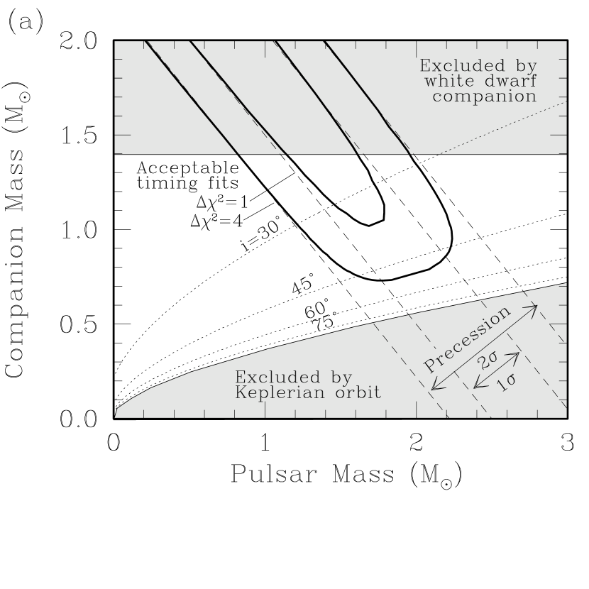
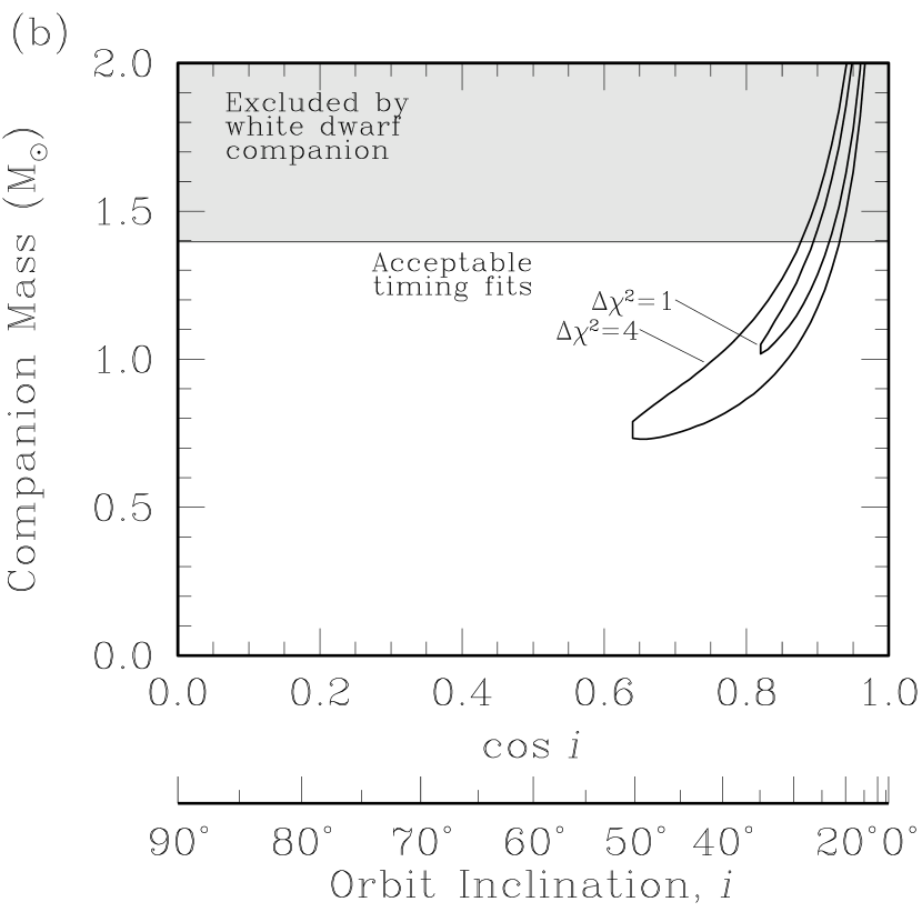
Figure 2: Values of pulsar mass, $m_{1}$, companion mass, $m_{2}$, and orbital inclination angle, $\cos i$, permitted by the Keplerian orbital elements, the relativistic timing model, and the assumption that the companion is a white dwarf. (a) Allowed values of $m_{1}$ and $m_{2}$. Dotted lines show selected values of constant $i$. (b) Allowed values of $\cos i$ and $m_{2}$. In both plots, the true values of the parameters must lie within the $\Delta\chi^{2}$ contours and outside the gray regions.

4.1 Keplerian Orbit

The masses and the inclination angle are related through the Keplerian mass function,

$$f_{1}(m_{1},m_{2},i)\equiv\frac{(m_{2}\sin{i})^{3}}{(m_{1}+m_{2})^{2}}=x^{3}\left(\frac{2\pi}{P_{b}}\right)^{2}\left(\frac{1}{T_{\odot}}\right)$$

$$=0.027026841\pm 0.000000004{\rm\,M}_{\odot},$$ (3)

where $i$ is the a priori unknown orbital inclination angle; $P_{b}$ is the orbital period; $x\equiv(a_{1}\sin{i})/c$ is the projected semi-major axis of the pulsar measured in light seconds, with $a_{1}$ the semi-major axis and $c$ the speed of light; and $T_{\odot}\equiv GM_{\odot}/c^{3}=4.925\times 10^{-6}$ s, with $G$ Newton’s gravitational constant. Since $\sin i\leq 1$, equation 3 can be rewritten to give an upper limit on $m_{1}$ in terms of $m_{2}$,

$$m_{1}\leq m_{2}^{3/2}f_{1}^{-1/2}-m_{2}.$$ (4)

This constraint is shown as the lower shaded region in Figure 2a.

4.2 Upper Limit on Companion Mass

The companion to the pulsar must be either a main sequence star, a neutron star, a black hole, or a white dwarf. The first possibility can be ruled out, as optical observations using the Hubble Space Telescope find no evidence that the secondary is a main sequence star (Camilo et al., to be published elsewhere). The second possibility can also be eliminated, since it is improbable that a double neutron star binary could have survived two supernova explosions and yet retained the small eccentricity of the PSR J0621+1002 system Portegies Zwart & Yungelson (1998). A pulsar-black hole binary is also unlikely to have such a circular orbit Lipunov et al. (1994). The companion must therefore be a white dwarf, and as such, its mass, $m_{2}$, must be lower than the Chandrasekhar limit, 1.4 M_⊙. This constraint is illustrated in Figure 2 as the upper shaded regions.

4.3 Relativistic Periastron Advance

The measured rate of periastron advance, $\dot{\omega}$, provides another relation between $m_{1}$ and $m_{2}$. For the PSR J0621+1002 system, we assume that nonrelativistic contributions to apsidal motion are negligibly small (see §4.6). The general relativistic interpretation of $\dot{\omega}$ then yields the combined mass of the stars,

$$M\equiv m_{1}+m_{2} = \left(\frac{P_{b}}{2\pi}\right)^{5/2}\left[\frac{(1-e^{2})\,\dot{\omega}}{3}\right]^{3/2}\left(\frac{1}{T_{\odot}}\right)$$ (5)

$$= 2.81\pm 0.30\,{\rm M}_{\odot}.$$

This constrains $m_{1}$ and $m_{2}$ to lie within the strips indicated by dashed lines in Figure 2a.

4.4 Shapiro Delay

According to general relativity, a pulse is delayed as it propagates through the gravitational potential well of the secondary. For a pulsar in a circular orbit, this so-called Shapiro delay is

$$\Delta t_{s}=-2\,m_{2}\,T_{\odot}\ln[1-\sin{i}\sin(\phi-\phi_{0})],$$ (6)

where $\phi$ is the orbital phase in radians and $\phi_{0}$ is the phase of the ascending node. For small inclination angles, the variation of $\Delta t_{s}$ over an orbit is nearly sinusoidal, and so it is indistinguishable from a minor increase in the projected orbital size, $x$. For edge-on orbits, with $i\approx 90^{\circ}$, the variation becomes strongly peaked at $\phi-\phi_{0}\approx\pi/2$, when the pulsar is behind the companion. This breaks the covariance with the Keplerian parameters, allowing measurement of Shapiro delay, and hence of $m_{2}$ and $i$.

Shapiro delay is not detected in the PSR J0621+1002 timing data. However, the magnitude of the effect is expected to be around $15\,\mu$s, which would make Shapiro delay easily detectable if the inclination angle were large. The fact that the delay is not observed therefore implies that the orbit is tilted substantially away from an edge-on orientation.

To explore the statistical limits that both the detection of periastron advance and the non-detection of Shapiro delay place on $i$ and $m_{2}$ (and hence on $m_{1}$), we analyzed the timing data over a grid of values in the ranges $0\leq\cos{i}\leq 1$ and $0\leq m_{2}\leq 2.0$ M_⊙. For each combination of $m_{2}$ and $\cos{i}$, we calculated the Shapiro delay parameters and the rate of periastron advance according to general relativity. We then performed a timing fit holding those quantities fixed while allowing all other parameters to vary. We recorded the resulting value of $\chi^{2}$ and its difference from the global minimum on the grid. Small departures in $\chi^{2}$ from the minimum signified the most likely configurations of $m_{2}$ and $\cos{i}$.

The solid contours in Figure 2a show the regions in which acceptable timing solutions were found. The interpretation of the contours is straightforward: within the area allowed by the precession measurement, the non-detection of Shapiro delay excludes solutions with “edge-on” orbits, and so the strip is truncated at low values of $\cos i$. Figure 2b shows that the inclination angle is constrained with a high degree of confidence to be less than 50^∘.

Following the statistically rigorous procedure described in Appendix A, we converted the $\chi^{2}$ differences to probabilities and derived probability distribution functions (PDFs) for $m_{1}$ and $m_{2}$. The analysis is restricted to timing solutions for which $m_{2}\leq 1.4$ M_⊙, in accordance with the discussion in §4.2. The PDFs of the pulsar and companion masses appear in Figure 3. They yield the maximum likelihood estimates

$$m_{1} = 1.70_{-0.29}^{+0.32}\rm{\,M}_{\odot}\ (\rm{68\%\ confidence})$$ (7)

$$= 1.70_{-0.63}^{+0.59}\rm{\,M}_{\odot}\ (\rm{95\%\ confidence})$$

for the pulsar and

$$m_{2} = 0.97_{-0.15}^{+0.27}\rm{\,M}_{\odot}\ (\rm{68\%\ confidence})$$ (8)

$$= 0.97_{-0.24}^{+0.43}\rm{\,M}_{\odot}\ (\rm{95\%\ confidence})$$

for the companion.

Note that the sum of the maximum likelihood estimates, 2.67 M_⊙, is less than the total system mass derived in equation 5 from periastron advance alone, 2.81 M_⊙. This is primarily a consequence of the upper limit on the companion mass, $m_{2}\leq 1.4$ M_⊙, which preferentially excludes solutions with high total mass, as can be seen in Figure 2a.

4.5 Interpretation of the Masses

A growing body of evidence finds that neutron stars in white dwarf-pulsar systems are not much more massive than those in double neutron star binaries, even though the secondaries must lose several tenths of a solar mass as they evolve toward white dwarfs. In particular, Thorsett & Chakrabarty (1999) find that the masses of neutron stars orbiting either white dwarfs or other neutron stars are consistent with a remarkably narrow Gaussian distribution, $m=1.35\pm 0.04$ M_⊙. While our measurement of the mass of PSR J0621+1002 is in statistical agreement with that result, the maximum likelihood value is suggestively high, allowing the possibility that a substantial amount of mass was transferred onto the neutron star.

Our estimate of the companion mass implies that the star is probably an ONeMg white dwarf and ranks it among the heaviest known white dwarfs in orbit around a pulsar. As van Kerkwijk & Kulkarni (1999) have pointed out, there are few massive white dwarfs, $m_{2}>1\,{\rm M}_{\odot}$, known to have evolved from a single massive progenitor star. They argue that the companion to PSR B2303+46, a young pulsar in an eccentric orbit, is such a white dwarf. Our timing of PSR J0621+1002 shows that its companion is similarly likely to have descended from a massive star, even though the histories of mass loss and accretion in the eccentric PSR B2303+46 binary, with no spin-up of the pulsar, and the circular PSR J0621+1002 binary, with significant spin-up, must have been very different.

Given the mass estimates, it seems likely that the PSR J0621+1002 system formed through a common envelope and spiral-in phase (Taam, King, & Ritter 2000; Tauris, van den Heuvel, & Savonije 2000). In this scenario, the companion originally had a mass of $5-7$ M_⊙, and the pulsar, initially in a wide orbit with a binary period of a few hundred days, spiraled in to its current orbit of $P_{b}=8.3$ under a drag force arising from its motion through the envelope. The same formation mechanism has been put forward for PSR J1454$-$5846, an object quite similar to PSR J0621+1002, with a 12.4-day orbital period, a 45.2-ms spin period, an eccentricity of 0.002, and a companion mass of $\sim$ 1.1 M_⊙ Camilo et al. (2001).

Figure 3: Probability distribution functions of (a) the pulsar mass and (b) the companion mass. The solid vertical lines mark the maximum likelihood values of the masses. The dashed vertical lines delimit 68% confidence regions; they represent the shortest widths along the mass axes that both enclose the peaks and contain 68% of the area under the curves. For the companion mass, the sharp falloff in the histogram reflects the assumption that $m_{2}\leq 1.40$ M_⊙.

4.6 Classical Periastron Advance

The above analysis assumed that the observed apsidal motion can be entirely attributed to relativity. In principle, however, apsidal motion could also be caused by distortions of the secondary star. Smarr & Blandford (1976) considered this possibility in the context of a potential white dwarf companion to the Hulse-Taylor binary pulsar, PSR B1913+16. Their analysis can also be applied to PSR J0621+1002. They found tidal deformation of the companion to contribute negligibly to $\dot{\omega}$ for PSR B1913+16. Since the apsidal advance per binary period due to tidal deformation scales as $a^{-5}$, where $a$ is the major axis, this effect can also be neglected in the wider PSR J0621+1002 system.

A potentially more important effect is rotational deformation, which becomes significant if the secondary is spinning rapidly. The precession rate due to rotation is

$$\dot{\omega}_{\rm rot}=nQ\left(1-{\textstyle\frac{3}{2}}\sin^{2}\theta+\cot i\sin\theta\cos\theta\cos\Phi_{0}\right)$$ (9)

Wex (1998), in which $n=2\pi/P_{b}$ and

$$Q=\frac{3k_{2}R_{2}^{5}\Omega^{2}}{a^{2}Gm_{2}(1-e^{2})^{2}},$$ (10)

where $k_{2}$, $R_{2}$, $\Omega_{2}$, and $m_{2}$ are the structure constant, radius, angular velocity, and mass of the secondary; $\theta$ is the angle between the angular momentum vector of the secondary and the angular momentum vector of the orbit; and $\Phi_{0}$ is the longitude of the ascending node in a reference frame defined by the total angular momentum vector (see Fig. 9 of Wex 1998). Neither $\theta$ nor $\Phi_{0}$ is known, so we must allow for all possible values in the ranges $0<\theta<\pi$ and $0<\Phi_{0}<2\pi$. Substituting PSR J0621+1002’s Keplerian orbital parameters, the formula can be written in the notation of Smarr & Blandford (1976):

$$\dot{\omega}_{\rm rot} = 0\fdg 000163\,{\rm yr}^{-1}\,\left(\frac{M_{\odot}}{m_{1}\!+\!m_{2}}\right)^{2/3}$$ (11)

$$\times \alpha_{6}\ \left(1-{\textstyle\frac{3}{2}}\sin^{2}\theta+\cot i\sin\theta\cos\theta\cos\Phi_{0}\right),$$

where $\alpha=2k_{2}R_{2}^{5}\Omega_{2}^{2}/(3Gm_{2})$ and $\alpha_{6}=\alpha/(10^{6}\,{\rm km^{2}})$. To gauge the largest value that $\dot{\omega}_{\rm rot}$ could attain, we will use limits on the masses and the orbital inclination angle from the relativistic analysis, recognizing that they would need to be modified should $\dot{\omega}_{\rm rot}$ be found significant. Our observations constrain $20^{\circ}<i<50^{\circ}$, so that $1.2<\cot i<2.7$ (see Fig. 2b), for which the maximum value of the geometric factor in equation 11 is 1.7, attained at $\theta=40^{\circ}$ and $\Phi_{0}=0$. Analyzing models of rotating white dwarfs, Smarr & Blandford (1976) found that $\alpha_{6}\lesssim 15$. Combining these restrictions with our measured value of total system mass, the precession due to rotation for PSR J0621+1002 can be as high as $\dot{\omega}_{\rm rot}\lesssim 0\fdg 0021$ yr^-1, about 20% of our observed value.

There is reason to believe that the classical contribution to the observed $\dot{\omega}$ is smaller than this. In most cases, a rotational deformation will induce a change in the projected semi-major axis of the orbit, $x=a_{1}\sin i/c$. Wex (1998) shows the rate of change to be

$$\frac{\dot{x}}{x}=nQ\cot i\sin\theta\cos\theta\sin\Phi_{0},$$ (12)

from which

$$\dot{\omega}_{\rm rot}=\frac{\dot{x}}{x}\,\left(\frac{1-\frac{3}{2}\sin^{2}\theta+\cot i\sin\theta\cos\theta\cos\Phi_{0}}{\cot i\sin\theta\cos\theta\sin\Phi_{0}}\right).$$ (13)

Thus, our observed upper limit of $|\dot{x}/x|<1.2\times 10^{-15}\,$ implies that $\dot{\omega}_{\rm{rot}}$ is no more than $1.2\times 10^{-15}\,{\rm rad}\,{\rm s}^{-1}=7\fdg 1\times 10^{-6}$ yr^-1 times a geometric factor. Unfortunately, certain special combinations of $i$, $\theta$, and $\Phi_{0}$ will make the geometric factor large. For this reason, we cannot definitively exclude the possibility that rotational precession contributes to the observed value of $\dot{\omega}$. For most cases, however, the geometric factor will be of order unity, and so the upper limit on $\dot{\omega}_{\rm rot}$ will be substantially smaller than our observed value of $\dot{\omega}$. Because of this, and because there is no reason to expect the secondary to be rapidly rotating, we have chosen to ignore $\dot{\omega}_{\rm rot}$ in our analysis of the pulsar and companion masses.

5 Density Irregularities in the ISM

5.1 Temporal DM Variations

Figure 4a shows the DM of PSR J0621+1002 calculated on individual days on which data were collected at Arecibo at both 430 and 1410  MHz. A DM drift as steep as 0.013 pc cm^-3 yr^-1 can be seen in the plot. If not properly modeled, such a gradient would shift the TOAs by up to 7 $\mu$s at 430 MHz over the 8-day pulsar orbit, a systematic effect significantly larger than the measurement uncertainties of the Arecibo TOAs. The DM gradient is among the largest ever detected in a pulsar outside a nebula Backer et al. (1993).

Figure 4: Dispersion measure as function of time, with $\Delta\rm{DM}=(\rm{DM}-36.6010)$. Vertical bars are $1\sigma$ uncertainties in the variations. (a) Measurements within a single day derived from dual-frequency observations at Arecibo. (b) Measurements derived from all TOAs averaged over intervals of 100 days, as indicated by horizontal bars.

Variations in the DM can be used to investigate inhomogeneities in the interstellar electron density. For this purpose, we modeled the DM as a series of step functions in time, as shown in Figure 4b. The width of the step intervals, 100 days, was a compromise between the goal of sampling DM as frequently as possible and the need for each segment to span enough multi-frequency data for the DM to be reliably calculated.

In Figure 4b, there appear to be discontinuities in the DM at 1997.4 and 1999.0. With a careful check of the data around these dates, we confirmed that the DM did indeed change by the amounts shown within the 100-day time resolution of the figure, and that the increase and decrease are not artifacts of binning the DM or of joining together data from different receivers and telescopes. However, the data do not allow us to distinguish between nearly instantaneous jumps in DM, as seen in the Crab pulsar signal (Backer, Wong, & Valanju 2000), and slower changes on a scale of 100 days. Given the rapid but apparently smooth variations in DM seen after 2000, we suspect the DM to be strongly but continuously varying at the earlier epochs as well.

5.2 Structure Function Analysis

The DM variations in Figure 4 result from the passage across the line of sight of density irregularities in the ionized ISM. The spatial structure of the irregularities can be discerned using the two-point structure function of the DM,

$$D_{\mathrm{DM}}(\tau)\equiv\left<[{\mathrm{DM}}(t+\tau)-{\mathrm{DM}}(t)]^{2}\right>,$$ (14)

where $\tau$ is the time lag between DM measurements and where the angular brackets denote ensemble averaging (e.g., Cordes et al. 1990). In a simple one-dimensional model where the line of sight cuts at the relative Sun-pulsar transverse velocity $V$ across a pattern of ISM irregularities that are “frozen in” a thin screen, and where the thin screen is midway between the Sun and the pulsar, the time lag is related to the spatial size $l$ of the density inhomogeneities through $l=V\tau/2$.

The structure function $D_{\rm DM}(\tau)$ can be approximated from the DM values at times $t_{i}$ through the unbiased estimator

$$\hat{D}_{\mathrm{DM}}(\tau)=\frac{1}{N(\tau)}\sum_{i=1}^{N(\tau)}[{\rm{DM}}(t_{i}+\tau)-{\rm{DM}}(t_{i})]^{2}-\sigma_{\mathrm{DM}}^{2},$$ (15)

where $N(\tau)$ is the number of DM pairs that enter into the summation at a given lag $\tau$ and where $\sigma_{\mathrm{DM}}$ is the mean uncertainty of the DM values. Figure 5 illustrates values of $\hat{D}_{\mathrm{DM}}(\tau)$ calculated this way for PSR J0621+1002. The uncertainties were computed by assuming Gaussian statistics for the fitted DM values and formally propagating their covariances through equation 15. We restrict $\tau$ to values for which $N(\tau)\geq 10$, thereby extending the lag from a minimum of 100 days to a maximum of 1300 days, about half the length of our full data span.

Figure 5: Structure function of DM variations of PSR J0621+1002 (Fig. 4). The points clearly do not all follow a single power law. As indicated by the dashed line, a power law was least-squares fitted to the first five points according to equation 17, yielding the spectral index, $\beta$.

5.3 Not a Simple Power Law

The structure function in Figure 5 presents a puzzle because it is not the simple power law that is predicted by standard theories of the ISM and that is seen in the direction of other pulsars. In the standard picture, a power law arises from the expectation that turbulence spreads energy from longer to shorter length scales. Accordingly, the spectrum of perturbations in the electron density is modeled in terms of the spatial frequency, $q=2\pi/l$, via

$$P(q)\propto q^{-\beta}$$ (16)

Rickett (1990). The relation is hypothesized to hold over some range of wave numbers, $q_{i}<q<q_{o}$; below some “inner scale” $q_{i}=2\pi/l_{i}$ and above some “outer scale” $q_{o}=2\pi/l_{o}$, various damping mechanisms are expected to cut off the turbulent energy flow. With the assumed linear relation between $l$ and $\tau$, the structure function becomes

$$D_{\mathrm{DM}}(\tau)=\left(\frac{\tau}{\tau_{0}}\right)^{\beta-2},$$ (17)

where $\tau_{0}$ is a normalization constant. The index $\beta$ is usually predicted to be near the Kolmogorov value for turbulence in neutral gases, $11/3$. Studies of DM variations in other pulsars have uncovered power laws with indices close to that value (Phillips & Wolszczan 1992; Kaspi, Taylor, & Ryba 1994; Cognard & Lestrade 1997).

The phase structure function in Figure 5 is obviously not a simple power law. It is not clear how to interpret this. A power law, marked by the dashed line, can be fit to the first five points in the plot. The slope of the line yields a spectral index, $\beta=3.28\pm 0.09$, that is reasonably close to the Kolmogorov value. At lags longer than 500 days, the power law fails to hold, although there is a hint of its reemergence at the longest lags. The flattening out of the structure function at 500 days is a direct consequence of the two sharp breaks in the DM time series (see Fig. 4b). If we take the Sun-pulsar transverse velocity to be $V=27$ km s^-1, then 500 days corresponds to a length of $l=V\tau/2=5.5\times 10^{13}{\rm{\,cm}}$, implying structure in the electron density power spectrum at this scale.

6 Conclusion

We have found substantial constraints on the masses of PSR J0621+1002 and its orbital companion. The pulsar mass is found to be $m_{1}=1.70^{+0.32}_{-0.29}$ M_⊙ (68% confidence). The lower end of this uncertainty range is near the canonical pulsar mass of 1.35 M_⊙, but the mass may also be several tenths of a solar mass higher, allowing the possibility that a substantial amount of material accreted onto the neutron star during the evolution of the system. The mass of the secondary, $m_{2}=0.97^{+0.27}_{-0.15}$ M_⊙ (68% confidence), makes it one of the heaviest known white dwarfs orbiting a pulsar.

Can the mass measurements be improved by continued timing observations? Unfortunately, post-Keplerian effects beyond those considered in this paper, such as orbital period decay, and gravitational redshift and time dilation, will not be detectable in the timing data for PSR J0621+1002 in the foreseeable future, so any improvement must come about through tighter measurements of $\dot{\omega}$ and Shapiro delay.

The uncertainty in the measurement of the total mass, $M=2.81\pm 0.30$ M_⊙, scales linearly with the uncertainty of $\dot{\omega}$, which in turn is inversely proportional to the time span over which data are collected. This has a simple explanation: the longer the time span of the observations, the more $\omega$ shifts, and so the easier it is to measure $\dot{\omega}$. The highest precision data used in this work—the annual Arecibo campaigns—were collected over two years. A similar campaign carried out several years in the future would shrink the uncertainty in $M$ by a factor of a few.

The pulsar and companion masses were further constrained by Shapiro delay. The precision of the Shapiro delay measurement (or limit) has no dependence on data span length, so its uncertainty is reduced only as $n^{-1/2}$, where $n$ is the number of observations. At best, a modest improvement could be made with existing radio telescope resources.

Appendix A Statistical Analysis of Pulsar and Companion Masses

The PDFs of the pulsar mass, $m_{1}$, and the companion mass, $m_{2}$, shown in §4.4 were calculated by least-squares fitting the TOAs to a timing model across a grid of $m_{2}$ and $\cos{i}$ values and analyzing the resulting changes in $\chi^{2}$. A formal derivation of the PDFs proceeds as follows. If $\chi^{2}_{0}$ is the global minimum on the grid, then each value of

$$\Delta\chi^{2}(m_{2},\,\cos{i})=\chi^{2}(m_{2},\,\cos{i})-\chi^{2}_{0}$$ (A1)

has a $\chi^{2}$ distribution with two degrees of freedom. It therefore maps to a Bayesian likelihood function,

$$p(\{t_{j}\}\,|\,m_{2},\cos{i})=\left(\frac{\textstyle{1}}{\textstyle{2}}\right)\,e^{-\Delta\chi^{2}/2},$$ (A2)

where $\{t_{j}\}$ stands for the data set. Accordingly, the joint posterior probability density of $m_{2}$ and $\cos{i}$ is

$$p(m_{2},\cos{i}\,|\,\{t_{j}\})=\frac{p(\{t_{j}\}|\,m_{2},\cos{i})}{p(\{t_{j}\})}\,p(m_{2},\cos{i}).$$ (A3)

The Bayesian “evidence”, $p(\{t_{j}\})$, is determined by normalizing the integral of $p(m_{2},\cos{i}\,|\{t_{j}\})$ over all grid points that are consistent with $m_{1}>0$, given the relationship among $m_{1}$, $m_{2}$ and $\cos{i}$ in the mass function in equation 3. As in all Bayesian investigations, a choice must be made for the prior, $p(m_{2},\cos{i})$. We selected the product of a uniform distribution on $0\leq m_{2}\leq m_{2,\,\mathrm{max}}$ and a uniform distribution on $0\leq\cos{i}\leq 1$. For the companion mass, the choice embodies our ignorance about the star; all that is known for certain is that it is a white dwarf, for which reason we set $m_{2,\,\mathrm{max}}=1.4$ M_⊙ (see §4.2). For the inclination angle, a flat distribution in $\cos{i}$ follows from the assumption that the orbital angular momentum vector has no preferred direction in space.

The PDF of $m_{2}$ is obtained by marginalizing equation A3 with respect to $\cos{i}$:

$$p(m_{2}|\{t_{j}\})=\int_{0}^{1}d(\cos{i})\,p(m_{2},\cos{i}\,|\{t_{j}\}).$$ (A4)

Similarly, the PDF of $m_{1}$ can be expressed as a double integral,

$$p(m_{1}\,|\{t_{j}\})=\int_{0}^{m_{2,\,\mathrm{max}}}dm_{2}\int_{0}^{1}d(\cos{i})\,$$

$$\times p(m_{1}\,|m_{2},\,\cos{i})\,p(m_{2},\cos{i}\,|\{t_{j}\}),$$ (A5)

where $m_{1}$ is guaranteed to be consistent with the mass function by setting

$$p(m_{1}|m_{2},\cos{i})=\delta\left[m_{1}-\left(\frac{(m_{2}\sin{i})^{3/2}}{f_{1}^{1/2}}-m_{2}\right)\right],$$ (A6)

with $\delta$ the Dirac function.

References

- Backer et al. (1993) Backer, D. C., Hama, S., Van Hook, S., & Foster, R. S. 1993, ApJ, 404, 636
- Backer, Wong, & Valanju (2000) Backer, D. C., Wong, T., & Valanju, J. 2000, ApJ, 543, 740
- Camilo et al. (2001) Camilo, F. et al. 2001, ApJ, 548, L187
- Camilo et al. (1996) Camilo, F., Nice, D. J., Shrauner, J. A., & Taylor, J. H. 1996, ApJ, 469, 819
- Cognard & Lestrade (1997) Cognard, I. & Lestrade, J.-F. 1997, A&A, 323, 211
- Cordes & Chernoff (1997) Cordes, J. M. & Chernoff, D. F. 1997, ApJ, 482, 971
- Cordes et al. (1990) Cordes, J. M., Wolszczan, A., Dewey, R. J., Blaskiewicz, M., & Stinebring, D. R. 1990, ApJ, 349, 245
- Damour & Deruelle (1986) Damour, T. & Deruelle, N. 1986, Ann. Inst. H. Poincaré (Physique Théorique), 44, 263
- Damour & Taylor (1991) Damour, T. & Taylor, J. H. 1991, ApJ, 366, 501
- Edwards & Bailes (2001) Edwards, R. T. & Bailes, M. 2001, ApJ, 553, 801
- Kaspi, Taylor, & Ryba (1994) Kaspi, V. M., Taylor, J. H., & Ryba, M. 1994, ApJ, 428, 713
- Kramer et al. (1999) Kramer, M., Xilouris, K. M., Camilo, F., Nice, D., Lange, C., Backer, D. C., & Doroshenko, O. 1999, ApJ, 520, 324
- Lipunov et al. (1994) Lipunov, V. M., Postnov, K. A., Prokhorov, M. E., & Osminkin, E. Y. 1994, ApJ, 423, L121
- Lyne et al. (1998) Lyne, A. G. et al. 1998, MNRAS, 295, 743
- Nice & Taylor (1995) Nice, D. J. & Taylor, J. H. 1995, ApJ, 441, 429
- Phillips & Wolszczan (1992) Phillips, J. A. & Wolszczan, A. 1992, ApJ, 385, 273
- Phinney & Kulkarni (1994) Phinney, E. S. & Kulkarni, S. R. 1994, ARAA, 32, 591
- Portegies Zwart & Yungelson (1998) Portegies Zwart, S. F. & Yungelson, L. R. 1998, A&A, 332, 173
- Rickett (1990) Rickett, B. J. 1990, ARAA, 28, 561
- Smarr & Blandford (1976) Smarr, L. L. & Blandford, R. 1976, ApJ, 207, 574
- Stairs et al. (2000) Stairs, I. H., Splaver, E. M., Thorsett, S. E., Nice, D. J., & Taylor, J. H. 2000, MNRAS, 314, 459
- Taam, King, & Ritter (2000) Taam, R. E., King, A. R., & Ritter, H. 2000, ApJ, 541, 329
- Tauris, van den Heuvel, & Savonije (2000) Tauris, T. M., van den Heuvel, E. P. J., & Savonije, G. J. 2000, ApJ, 530, L93
- Taylor & Cordes (1993) Taylor, J. H. & Cordes, J. M. 1993, ApJ, 411, 674
- Thorsett & Chakrabarty (1999) Thorsett, S. E. & Chakrabarty, D. 1999, ApJ, 512, 288
- Toscano et al. (1999) Toscano, M., Sandhu, J. S., Bailes, M., Manchester, R. N., Britton, M. C., Kulkarni, S. R., Anderson, S. B., & Stappers, B. W. 1999, MNRAS, 307, 925
- van den Heuvel (1994) van den Heuvel, E. P. J. 1994, A&A, 291, L39
- van Kerkwijk & Kulkarni (1999) van Kerkwijk, M. & Kulkarni, S. R. 1999, ApJ, 516, L25
- Wex (1998) Wex, N. 1998, MNRAS, 298, 997