The Fundamental Plane of Ellipticals:
I. The Dark Matter Connection

Abstract

We show that the small scatter around the Fundamental Plane (FP) of massive elliptical galaxies can be used to derive important properties of their dark and luminous matter. The central velocity dispersion $\sigma_{0}$, appearing in (e.g.) the Fundamental Plane, is linked to photometric, dynamical and geometrical properties of (luminous and dark) matter. We find that, inside the effective radius $R_{e}$, the matter traced by the light must largely dominate over the dark matter (DM), in order to keep the ellipticals close enough to the FP. This recalls analogous findings for spiral galaxies.

In particular we also find that cuspy DM distributions, as predicted by numerical simulations in $\Lambda$CDM cosmology, are unable to explain the very existence of the FP; in fact, according to this theory, the structural properties of dark and luminous matter are so interwoven that a curved surface is predicted in the log–space ($\sigma_{0}$, $R_{e}$, $L$), rather than a plane. In order to agree with the FP, CDM halos must have concentrations parameters in the range of $5-9$ (i.e. values significantly lower than the current predictions).

Assuming a more heuristic approach and allowing for cored DM halos, we find that the small intrinsic scatter of the FP yields to i) an average value for the dark–to–light–traced mass ratio inside the length–scale of light $R_{e}$ of about $0.3$, ii) a mass–to–light ratio of the matter traced by the light increasing with spheroid luminosity: $M_{sph}/L_{r}\propto L_{r}^{0.2}$ in Gunn–$r$ band, with a value of $5.3$ at $L_{\ast r}\equiv 2.7\times 10^{10}L_{r\odot}$.

1 Introduction

In the hierarchical scenario, dark matter (DM) halos have driven, from a variety of initial conditions, a dissipative infall of baryons and formed the galactic systems we observe today (White and Rees, 1978). Thus, we expect that DM halos exist within and surrounding any galaxy, regardless of its luminosity and morphological type. This prediction had overwhelming confirms for disk galaxies, due to the existence of good dynamical tracers and their intrinsic simple geometry (see Persic and Salucci, 1997). Elliptical galaxies (E’s), however, are much more complicated objects, due to their 3–dimensional shape, stellar orbital structure and velocity dispersion anisotropy. These factors have made ambiguous the interpretation of observational data.

A number of different mass tracers have been used to probe the gravitational potential in tenth of E’s and derive their mass distribution: integrated stellar absorption spectra, X–ray emission from hot gas, rotating gas disks, motions of globular clusters or satellite galaxies and, in last years, weak gravitational lensing. As result, the presence of dark matter in E’s, especially in the external regions ($\,\lower 2.0pt\hbox{${>\atop\hbox{\raise 4.0pt\hbox{$\sim$}}}$}\,10$ kpc), is proven (e.g. Loewenstein and White, 1999). On the other hand, a kinematical modeling of the inner regions (i.e. within the half–luminosity “effective” radius $R_{e}$), has been performed for only a small number of ellipticals (e.g. van der Marel, 1991; Saglia et al. 1992, 1993; Bertin et al., 1994; Kronawitter et al., 2000; Gerhard et al., 2001); the results point to a tendency for moderate dark matter amounts inside $R_{e}$.

Since its discovery, the “Fundamental Plane” (Djorgovski & Davis, 1987; Dressler et al., 1987) has been one of the main tools to investigate E’s properties: effective radius $R_{e}$, central velocity dispersion $\sigma_{0}$ and mean effective surface brightness $I_{e}$ of spheroidal galaxies are linearly related in the logarithmic space and galaxies closely cluster on a plane, with a surprisingly low orthogonal scatter. To explain these linear relations between photometric and dynamical quantities in log–space, most studies on the Fundamental Plane (FP) have considered models in which the mass is distributed parallel to light. However, in presence of non–baryonic dark matter, this hypothesis is an obvious oversimplification and, at least, unjustified. Indeed, this would a priori require either: i) dark and luminous component are distributed according the same profile, thus revealing a similarity of properties and behavior which seems very unlikely or ii) the dark matter component is always negligible with respect to the luminous matter.

Within the above framework, in this paper we address the following issues:

• to derive the relation between the central velocity dispersion $\sigma_{0}$ and the mass distribution parameters, including the effect of a dark matter halo. In particular, we assume a spherical model with an isotropic luminous component and a dark halo, more diffuse than the spheroid,

• to reproduce the observed Fundamental Plane and, therefore, to constrain the mass distribution in E’s,

• to discuss the results in the light of Cold Dark Matter predictions.

Considering elliptical galaxies as two–components systems, complementary strategies are possible. One chooses a distribution function for both components and then imposes specific constraints from the observations. The other includes the ordinary stellar component (or, better, any traced by light (TBL) mass component) in a frozen spherical halo. The former approach is helpful in exploring the self–consistency of the dynamical configuration (e.g. Ciotti, 1999). The latter, we will adopt in this paper, has the advantage of providing a simpler connection between observational quantities and the parameters of the mass model.

The outline of this paper is the following: in §2 we describe two–components models, whose mass distributions are shown in §3. In §4 we derive and discuss the velocity dispersion (line–of–sight profile and central value) predicted by the mass models we consider. In §5, we introduce the data, fit the models to the Fundamental Plane and discuss the results. Finally, conclusions are presented in §6. Throughout the following work, we assume, where needed, a flat $\Lambda$CDM Universe, with $\Omega_{m}=0.3$, $\Omega_{\Lambda}=0.7$, $h=0.7$ and $\sigma_{8}=1.0$.

2 The velocity dispersion in the 2-components mass models

The observed velocity dispersion and, in particular, the central velocity dispersion $\sigma_{0}$ is a fundamental dynamical property related to the gravitational potential of both the dark halo and the TBL component (sometime, we call the “luminous stellar spheroid” by this way, to recall the possible existence of a number of BH’s and/or an amount of non–baryonic DM, perfectly mixed with the luminous stellar matter). Let us start by assuming a spherical and non–rotating stellar system, with the stellar velocity dispersion which is the same in all directions perpendicular to a given radial vector. If $\sigma_{r}^{2}(r)$ denotes the stellar velocity dispersion along the radial vector and $\sigma_{\theta}^{2}(r)$ the dispersion in the perpendicular directions, the Jeans hydrodynamic equation for the mass density traced by the light $\rho_{sph}(r)$ in the radial direction reads (Binney and Tremaine, 1987):

$$\frac{d\rho_{sph}(r)\sigma_{r}^{2}(r)}{dr}+\frac{2\ \beta(r)\rho_{sph}(r)\sigma^{2}_{r}(r)}{r}=-\frac{GM(r)}{r^{2}}\rho_{sph}(r)$$ (1)

with the boundary condition $\rho_{sph}(r)\sigma^{2}_{r}(r)\rightarrow 0$ for $r\rightarrow\infty$. In eq.(1), the parameter $\beta(r)\equiv 1-\sigma_{\theta}^{2}(r)/\sigma_{r}^{2}(r)$ describes the anisotropy degree of the velocity dispersion at each point, with $\beta=1,0,-\infty$ for completely radial, isotropic and circular orbit distributions, respectively.

Dynamical analysis of ellipticals exclude substantial amount of tangential anisotropy and find $\beta(\,\lower 2.0pt\hbox{${<\atop\hbox{\raise 4.0pt\hbox{$\sim$}}}$}\,R_{e})\simeq 0.1-0.2$ (e.g. Matthias and Gerhard, 1999; Gerhard et al., 2001; Koopmans and Treu, 2002) for objects of different luminosities. For reasons of simplicity, then, in calculating the central velocity dispersion to be used for statistical studies over a large sample of galaxies, we assume an isotropic velocity dispersion tensor: $\beta=0$.

Eq.(1) connects the spatial velocity dispersion of the component traced by the light to its density profile and to the total matter distribution $M(r)=M_{sph}(r)+M_{h}(r)$. Under the hypothesis of isotropy, the above equation assumes the well–known integral form, in which we single out the halo term:

$$\sigma_{r}^{2}(r)=\frac{G}{\rho_{sph}(r)}\int_{r}^{\infty}\frac{\rho_{sph}(r^{\prime})M(r^{\prime})}{r^{\prime 2}}\ dr^{\prime}\equiv\sigma_{r;sph}^{2}(r)+\sigma_{r;h}^{2}(r)$$ (2)

As external observers of galaxies, we measure only projected quantities. Let $R$ be the projected radius and $\Sigma(R)$ the surface stellar mass density. As usual, we take into account that mass density and the spatial velocity dispersion are related to the surface mass density $\Sigma(R)$ and to the projected velocity dispersion $\sigma_{P}(R)$ by the two Abel integral equations for the quantity $\rho_{sph}$ and $\rho_{sph}\sigma_{r}^{2}$. Then, a second step, consisting in a further integration along the line of sight, allows us to obtain the (observed) velocity dispersion profile $\sigma_{P}(r)$:

$$\sigma_{P}^{2}(R)=\frac{2}{\Sigma(R)}\ \int_{R}^{\infty}\ \frac{\rho_{sph}(r)\ \sigma_{r}^{2}(r)\ r}{\sqrt{r^{2}-R^{2}}}\ dr\equiv\sigma_{P;sph}^{2}(R)+\sigma_{P;h}^{2}(R)$$ (3)

where $\Sigma(R)=\int_{R}^{\infty}\ [2\ r\ \rho_{sph}(r)/(r^{2}-R^{2})^{1/2}]\ dr$.

As spectro–photometric observations are performed through an aperture, let us define $\sigma_{A}(R_{A})$ as the luminosity–weighted average of $\sigma_{P}$ within a circular aperture of radius $R_{A}$:

$$\sigma_{A}^{2}(R_{A})=\frac{2\pi}{L(R_{A})}\ \int_{0}^{R_{A}}\ \sigma_{P}^{2}(R)\ I(R)\ R\ dR\equiv\sigma_{A;sph}^{2}(R_{A})+\sigma_{A;h}^{2}(R_{A})$$ (4)

where $I(R)$ is the surface brightness profile $I(R)=\Sigma(R)/\Upsilon$ (assuming the stellar mass–to–light ratio $\Upsilon$ constant with radius) and $L(R_{A})=2\ \pi\ \int_{0}^{R_{A}}I(R)\ R\ dR$ is the aperture luminosity.

The dynamical quantity in the Fundamental Plane is the “central” velocity dispersion $\sigma_{0}$, which, observationally, corresponds to the projected velocity dispersion luminosity–weigthed within the aperture of the observations. The velocity dispersion data are to be brought to a common system, independent of the telescope and galaxy distance: this is done by correcting them to the same aperture of $R_{e}/8$ (Jørgensen et al., 1996), which is typical of measurements of nearby galaxies. Therefore, we compare model and observations by calculating $\sigma_{0}$ as the luminosity–weighted $\sigma_{P}(R)$ within $R_{A}=1/8\ R_{e}$.

The resulting velocity dispersion profiles, $\sigma_{r}(r)$, $\sigma_{P}(R)$ and $\sigma_{A}(R_{A})$, can be all expressed as the sum of two terms (eqs. 2, 3 and 4): the first one is due to the self–gravity of the spheroid traced by the star light (labelled by $sph$); the second one (labelled by $h$) is due to the effect of the luminous–dark matter gravitational interaction and, therefore, it charges relevance according the characteristics of the DM distribution.

3 The mass distribution

3.1 The distribution of the mass traced by light

We describe the component traced by the star light by means of a Hernquist (1990) spherical density distribution, that is a good approximation to the de Vaucouleurs $R^{1/4}$ law (de Vaucouleurs, 1948) when projected and, at the same time, allows analytical calculations:

$$\rho_{sph}(r)=\frac{M_{sph}}{2\pi}\frac{k\ R_{e}}{r\ (r+k\ R_{e})^{3}}$$ (5)

where $M_{sph}$ is the total mass traced by the star light and $k\simeq 0.55$. The mass profile derived from eq.(5) is:

$$M_{sph}(r)=M_{sph}\frac{(r/R_{e})^{2}}{(r/R_{e}+k)^{2}}$$ (6)

The Hernquist functional form, of course, cannot reproduce the fine features of the surface brightness profile (e.g. boxy isophotes, small variations in slope); neverthless, it is sufficient for our aims, since we will just consider large scale properties in the mass distribution of objects belonging to a large E’s sample.

3.2 The DM distribution: $\Lambda$CDM halos

N–body simulations of hierarchical collapse and merging of CDM halos have shown that gravity, starting from scale–free initial conditions, produces an universal density profile that, for $r\rightarrow\ 0$, varies with radius as $r^{-\alpha}$, with $\alpha\sim 1-2$ (e.g. Navarro, Frenk & White, 1997, hereafter NFW; Fukushige and Makino, 1997; Moore et al., 1998; Ghigna et al., 2001), weakly dependent on the cosmological model. We adopt the well–known NFW halo density profile:

$$\rho_{NFW}(r)=\frac{\rho_{s}}{(r/r_{s})(1+r/r_{s})^{2}}$$ (7)

where $r_{s}$ is the inner characteristic length–scale, corresponding to the radius where the logarithmic slope of the profile is $-2$. It results convenient to write the NFW mass profile as:

$$M_{NFW}(r)=M_{vir}\ \frac{A(r,r_{s})}{A(c,r_{s}/R_{e})}$$ (8)

where $A(x,y)\equiv\ln(1+x/y)-(1+y/x)^{-1}$ for any pair of variables $(x,y)$. The concentration parameter is defined as $c\equiv r_{vir}/r_{s}$; $r_{vir}$ and $M_{vir}$ are, respectively, the halo virial radius and mass. The definition of the virial radius is strictly within the framework of the standard dissipationless spherical collapse model (SCM); however, also in more realistic hierarchical models, it provides a measure of the boundary of virialized region of halos (Cole and Lacey, 1996).

Considering a dark halo at redshift $z$, the virialized region is the sphere within which the mean density is $\Delta_{vir}(z)$ times the background universal density at that redshift ($\rho_{bkg}=\rho_{c}\ (1+z)^{3}$, with $\rho_{c}$ the critical density for closure at $z=0$). The virial mass is defined as: $M_{vir}\equiv\frac{4}{3}\ \pi\ \Delta_{vir}(z)\ \rho_{bkg}\ r_{vir}^{3}$, with the virial overdensity $\Delta_{vir}$ being a function both of the cosmological model and the redshift: for the family of flat cosmologies ($\Omega_{\rm m}+\Omega_{\Lambda}=1$), it can be approximated by (Bryan and Norman, 1998): $\Delta_{vir}(z)\simeq 18\pi^{2}+82(\Omega(z)-1)-39(\Omega(z)-1)^{2}/\Omega(z)$. From the above equations, we derive:

$$r_{vir}=0.142\ \Delta_{vir}(z)^{-1/3}(1+z)^{-1}\left(\frac{M_{vir}}{M_{\odot}}\right)^{1/3}\ h^{-2/3}\ {\rm kpc}$$ (9)

A fundamental result of CDM theory is that the halo concentration well correlates with the virial mass: low–mass halos are denser and more concentrated than high–mass halos (Bullock et al., 2001; Cheng and Wu, 2001; Wechsler et al., 2002) in that, in average, they collapsed when the Universe was denser. Numerical experiments by Wechsler et al. (2002) for a population of halos identified at $z=0$ show that:

$$c(M_{vir})\simeq c_{11}\ \left(\frac{M_{vir}}{10^{11}\ M_{\odot}}\right)^{-0.13},$$ (10)

with $c_{11}\simeq 20.8$. The Poisson error for galactic halos in the mass range $M_{vir}\,\lower 2.0pt\hbox{${<\atop\hbox{\raise 4.0pt\hbox{$\sim$}}}$}\,10^{11-13}M_{\odot}$ is less than 10$\%$ and, virtually, no halo is found with $c<12$.

This is the first mass model we consider here: it is composed by a stellar bulge with a Hernquist profile embedded in a spherical dark NFW halo (hereafter H+NFW model). We neglect the effects of a possible adiabatic coupling between baryons and dark matter because it has the effect of increasing the DM density inside $R_{e}$ by adiabatic compression and, then, of worsening the fit to the data (see $\S$5.3.1). The “total” dark–to–TBL mass ratio, defined as $\Gamma_{vir}\equiv M_{vir}/M_{sph}$ is a crucial parameter of the mass model. Both BBN predictions about the primordial DM–to–baryons ratio and CMB anisotropy observations point at a lower limit for $\Gamma_{vir}$ of $\simeq 8$.

3.3 The DM distribution: cored halos

In last years, studies of high resolution rotation curves of spiral and dwarf galaxies casted doubts on the presence of the central cusps predicted by cosmological simulations of DM halos. Actually, the observational results suggest that dark halos are more diffuse than the luminous component and their densities flatten at small radii, whereas the stellar distribution peaks towards the centre (e.g. Moore, 1994; Flores and Primack, 1994; Burkert, 1995; de Battista and Sellwood, 1998; Salucci and Burkert, 2000; de Block, McGaugh and Rubin, 2001; Borriello and Salucci, 2001).

An useful analytic form for halos with soft cores has been proposed by Burkert (1995) for dwarf galaxies and, then, was extended to the whole family of spirals by Salucci and Burkert (2000):

$$\rho_{B}(r)=\frac{\rho_{0}}{(1+r/r_{0})[1+(r/r_{0})^{2}]}$$ (11)

This profile is characterized by a density–core of extension $r_{0}$ and value $\rho_{0}$, while it resembles the NFW profile at large radii. From eq.(11) the mass profile reads:

$$M_{B}(r)=M_{e}\ \frac{B(r,r_{0})}{B(1,r_{0}/R_{e})}$$ (12)

where, for any pair of variables $(x,y)$, $B(x,y)\equiv-2\arctan(x/y)+2\ln(1+x/y)+\ln[1+(x/y)^{2}]$ and $M_{e}$ is the dark mass within $R_{e}$. Then, in analogy of spiral galaxies, we propose a mass model consisting of a Hernquist bulge plus a Burkert dark halo (hereafter H+B model). This is the second mass model we investigate in this paper; let us notice that, in this case, the halo mass distribution is characterized by two free parameters: the dark–to–TBL mass ratio within the effective radius $\Gamma_{e}\equiv M_{DM}/M_{sph}\mid_{R_{e}}$ and the halo core radius in units of the effective radius $r_{0}/R_{e}$. We assume $r_{0}\,\lower 2.0pt\hbox{${>\atop\hbox{\raise 4.0pt\hbox{$\sim$}}}$}\,R_{e}$ to ensure a constant DM density in the region where the stars reside: otherwise the model would essentially coincide with the NFW one.

It is worth noticing that the Burkert profile is purely heuristic and featureless in the optical regions of galaxies; as a consequence, unless data at large radii are available, it is not possible to determine the halo virial radius and the total galaxy mass.

4 Mass–velocity dispersions relations for cuspy and cored models

We compute the velocity dispersion profiles, including the effect of a spherical dark halo, for both H+NFW and H+B cases. We resolve eq.(2), eq.(3) and eq.(4) by assuming the density/mass profiles of eq.(5), eq.(6) and eq.(8) in H+NFW case and of eq.(5), eq.(6) and eq.(12) in the H+B one. The detailed calculus in given in Appendix.

 

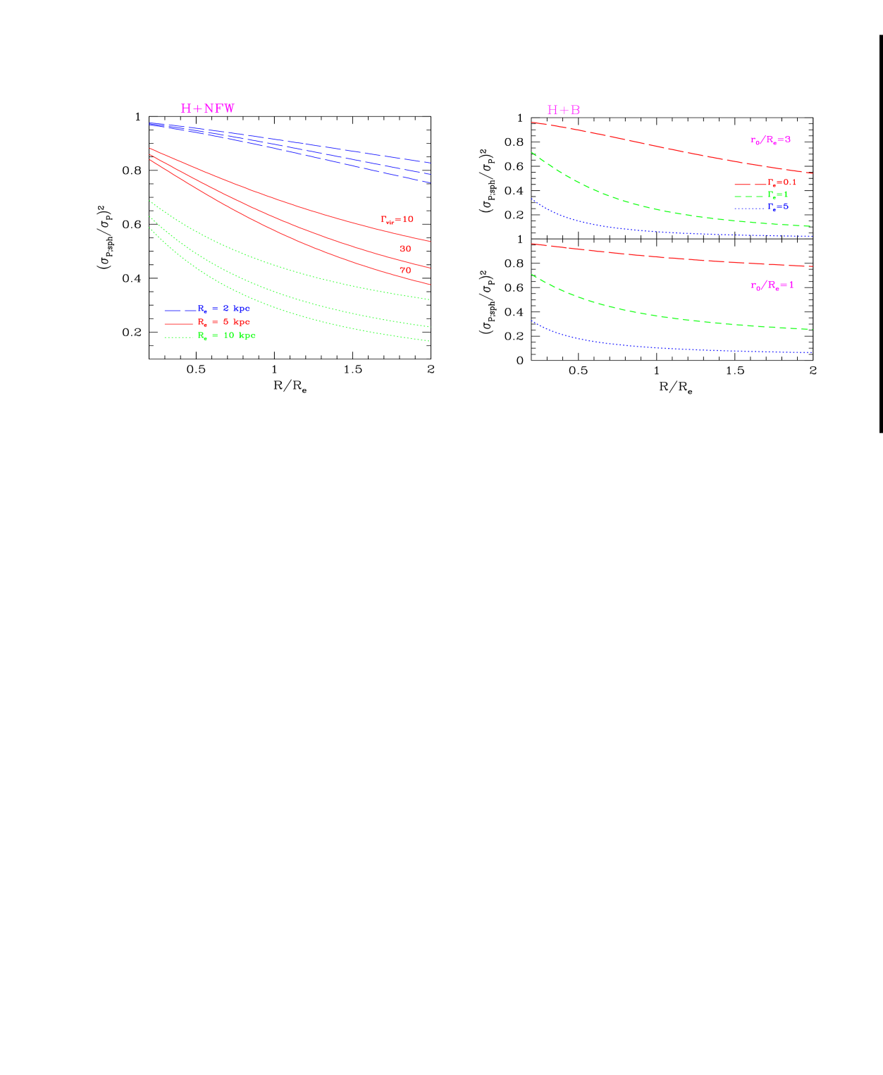
Figure 1: Line–of–sight velocity dispersion due to the spheroid (in units of total velocity dispersion) as a function of radius for: left) H+NFW case (different values of $R_{e}$ and $\Gamma_{vir}$ are indicated); right) H+B case (different values of $r_{0}/R_{e}$ and $\Gamma_{e}$ are indicated).

In Fig.1 (left) we show, for H+NFW models, the radial profile of the quantity $\sigma^{2}_{P;sph}/\sigma^{2}_{P}$, the line–of–sight velocity dispersion due to the TBL component, in units of the total l.o.s. velocity dispersion. We take $M_{sph}=2\times 10^{11}M_{\odot}$; however, the mass dependence is very weak and the curves in Fig.1 (left) are well representative of those with stellar masses in the range $\sim 5\times 10^{9}-10^{12}M_{\odot}$. We consider different plausible values for the total dark–to–TBL mass ratio $\Gamma_{vir}$ and $R_{e}$. Let us notice that, once we fix the total halo mass $M_{vir}\equiv\Gamma_{vir}\cdot M_{sph}$, the halo characteristic radius $r_{s}$ is completely determined via the $c-M_{vir}$ relationship: therefore, different curves in Fig.1 (left) correspond to $2\,\lower 2.0pt\hbox{${<\atop\hbox{\raise 4.0pt\hbox{$\sim$}}}$}\,r_{s}/R_{e}\,\lower 2.0pt\hbox{${<\atop\hbox{\raise 4.0pt\hbox{$\sim$}}}$}\,30$.

We realize that the contribution of a CDM halo to the velocity dispersion can be large ($\sim 50\%$) even at small radii $R\,\lower 2.0pt\hbox{${<\atop\hbox{\raise 4.0pt\hbox{$\sim$}}}$}\,R_{e}/2$, in galaxies with large effective radii and/or small values of $r_{s}/R_{e}$, indipendently of the value of $\Gamma_{vir}$.

 

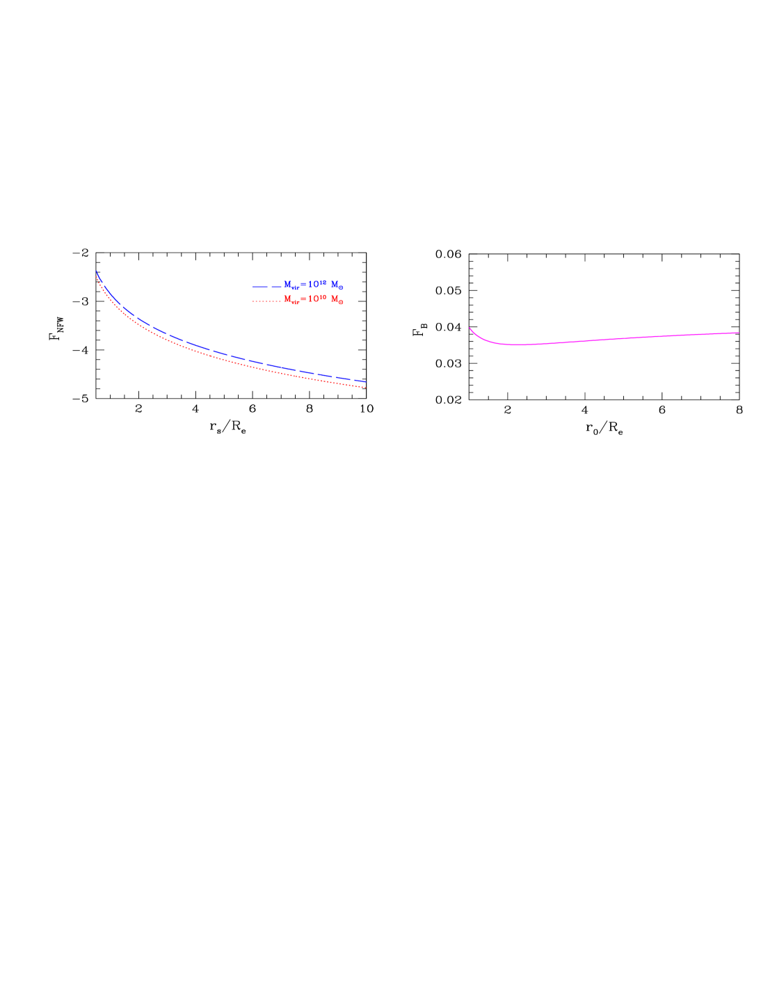
Figure 2: The functions $F_{\rm NFW}$ and $F_{\rm B}$ entering the expression of $\sigma_{0}$, for H+NFW model (left) and H+B model (right).

In Fig.1 (right) we plot the TBL–to–total l.o.s. velocity dispersion ratio for H+B models, for different values of the parameters $r_{0}/R_{e}$ and $\Gamma_{e}$. Notice that the profiles just depend on these parameters and it is not necessary to assume specific values both for $M_{sph}$ or $R_{e}$. The main consequence of the smooth halo profile in the H+B model is that the halo contribution to $\sigma_{P}(R)$ is low at small $R$, even for models with a relevant amount of DM in the central region (e.g. $\sigma^{2}_{P;sph}/\sigma^{2}_{P}\sim 80\%$ at $R_{e}/3$ when $\Gamma_{e}=1$). The velocity dispersion in the central regions is more directly connected to the properties of the TBL mass distribution.

The relationship of the spheroid mass with central velocity dispersion $\sigma_{0}$ and the effective radius $R_{e}$ depends on the DM mass distribution. Recalling that $\sigma_{0}\equiv\sigma_{A}(R_{e}/8)$, we find:

$$\sigma_{0}^{2}=(0.174+\Gamma_{vir}\ F_{NFW})\ \frac{G\ M_{sph}}{R_{e}}\ \ \ \ \ \ \ \ \ \ \ \ \ \ \ {\rm H+NFW}$$ (13)

$$\sigma_{0}^{2}=(0.174+\Gamma_{e}\ F_{B})\ \frac{G\ M_{sph}}{R_{e}}\ \ \ \ \ \ \ \ \ \ \ \ \ \ \ \ \ \ \ \ \ {\rm H+B}$$ (14)

where $F_{\rm NFW}$ and $F_{\rm B}$ are shown in Fig.2. $F_{\rm NFW}$ depends on $r_{s}(M_{vir})/R_{e}$ and, very weakly, on $M_{vir}\equiv\Gamma_{vir}\cdot M_{sph}$. The term in the r.h.s. of eqs.(13) and (14) shows that, according to the values of the model parameters, $\sigma_{0}$ could be strongly affected by the DM gravitational potential, so that the derivation of the spheroidal mass from obsevational properties critically depends on the actual DM mass profile. This is shown in (Fig.3, left), where we plot the TBL–to–total $\sigma^{2}_{0}$, assuming $M_{sph}=2\times 10^{11}M_{\odot}$ and different model parameters: the TBL contribution to $\sigma^{2}_{0}$ is under dominant also at small $r_{s}/R_{e}$ and becomes almost negligible for $r_{s}/R_{e}\,\lower 2.0pt\hbox{${<\atop\hbox{\raise 4.0pt\hbox{$\sim$}}}$}\,1$ and $\Gamma_{vir}\,\lower 2.0pt\hbox{${>\atop\hbox{\raise 4.0pt\hbox{$\sim$}}}$}\,30$.

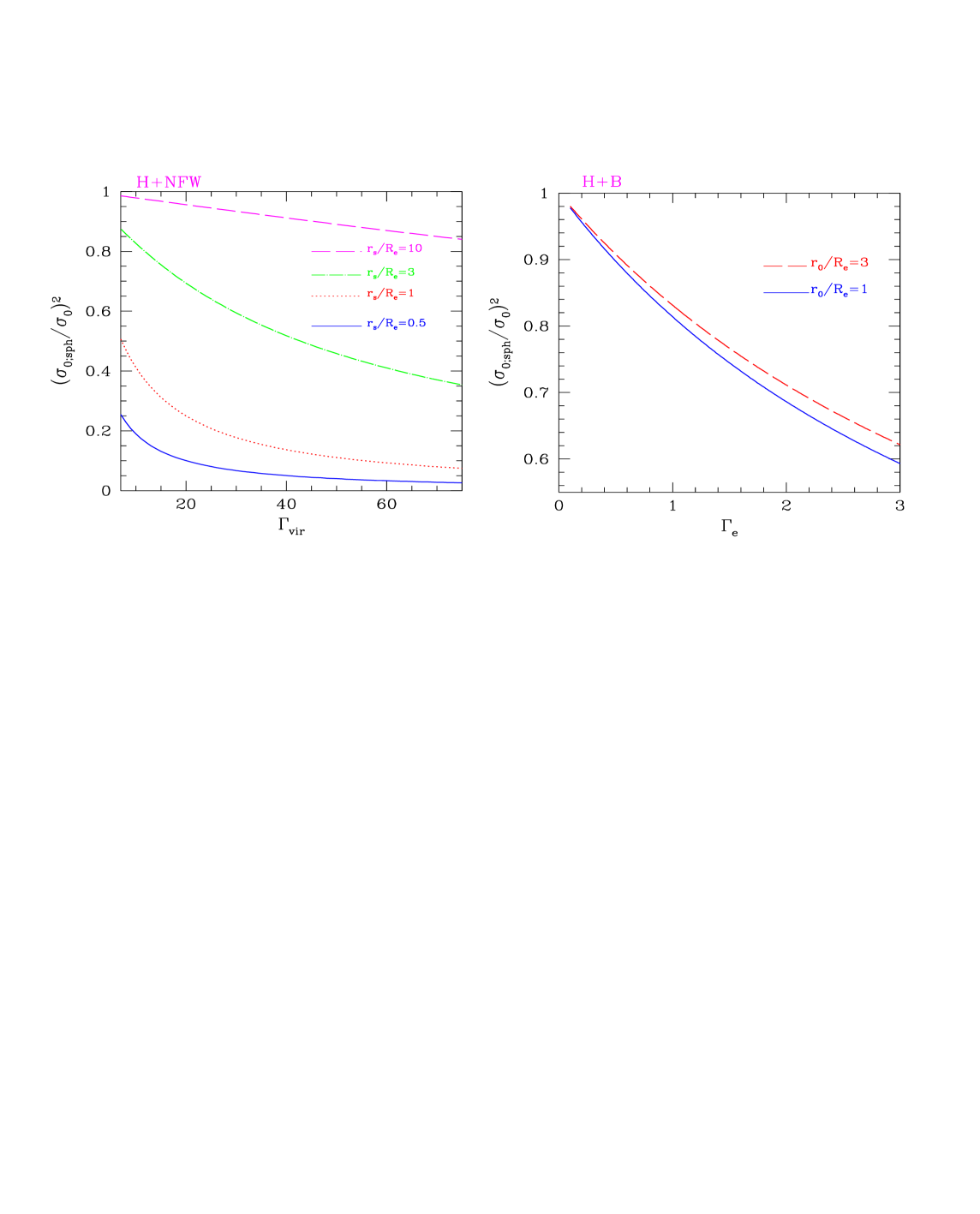
Figure 3: The TBL mass component contribution to $\sigma_{0}$ for different models parameters: left) H+NFW predictions for $M_{sph}=2\times 10^{11}M_{\odot}$, as function of $\Gamma_{vir}$ and for different $r_{s}/R_{e}$; right) H+B predictions, as function of the parameters $\Gamma_{e}$ and $r_{0}/R_{e}$.

In H+B mass models, $F_{\rm B}$ weakly depends on $r_{0}/R_{e}$, so that we can assume $F_{\rm B}\simeq 3.6\times 10^{-2}$; the TBL contribution to $\sigma^{2}_{0}$ (Fig.3, right) remains the dominant one, even for an amount of DM within $R_{e}$ comparable to the luminous one. Moreover, from eq.(14) we infer that, for cored configurations (i.e. with $r_{0}>R_{e}$), $\sigma_{0}$ is weakly dependent on the DM internal amount ($F_{\rm B}$ is of the order of $10^{-2}$): as a matter of fact, it just increases of $\sim 30\%$ when $\Gamma_{e}$ varies of a factor 3. This is a natural consequence of the smoothness of the dark matter distribution with respect to the more concentrated distribution of the luminous spheroid.

5 Fitting mass models to the Fundamental Plane

5.1 The Sample

We build the data sample from several works by Jørgensen, Franx & Kjaergaard (hereafter JFK). They provide spectroscopy and multicolour CCD surface photometry of E/S0 galaxies in nearby clusters. The photometric data are from JFK (1992) and (1995a) in Gunn–$r$, their passband with the largest quantity of data. The spectroscopic measurements are taken from JFK (1995b) and references therein. Out of the whole JFK sample, we selected a homogeneous subsample of 221 E/S0 galaxies in 9 clusters, including Coma, whose properties are shown in electronic form in Tab.1 at the URL: www.sissa.it/ap/ftp. In particular, we rejected spiral, interacting, peculiar and field galaxies (due to the greater uncertainty of their distance). For each cluster, we adopt the distance derived in JFK (1996). The FP r.m.s. scatter is 0.084 in $\log R_{e}$ (this is equivalent to a $\sim 17\%$ uncertainty in galaxy distances that, then, could be the main scatter contributor). Typical measurement errors are $\Delta\log R_{e}=\pm 0.045$, $\Delta\log I_{e}=\pm 0.064$, $\Delta\log\sigma_{0}=\pm 0.036$, and $\Delta\log L_{r}=\pm 0.036$, maybe large enough to imply that the FP is free from an intrinsic scatter.

The statistical distributions of effective radius, ellipticity at $R_{e}$, observed central velocity dispersion and Gunn–$r$ luminosity of the selected galaxies are shown in Fig.4. It is worth noticing that the sample galaxies are distributed around $L_{\ast}=2.7\times 10^{10}L_{r\odot}$, the characteristic luminosity of the ellipticals luminosity function in $r$–band (Blanton et al., 2001) and that most of the objects have little/moderate ellipticity ($<\epsilon>=0.29\pm 0.17$) and then, a reasonably spherical stellar distribution.

5.2 Forcing models to the Fundamental Plane

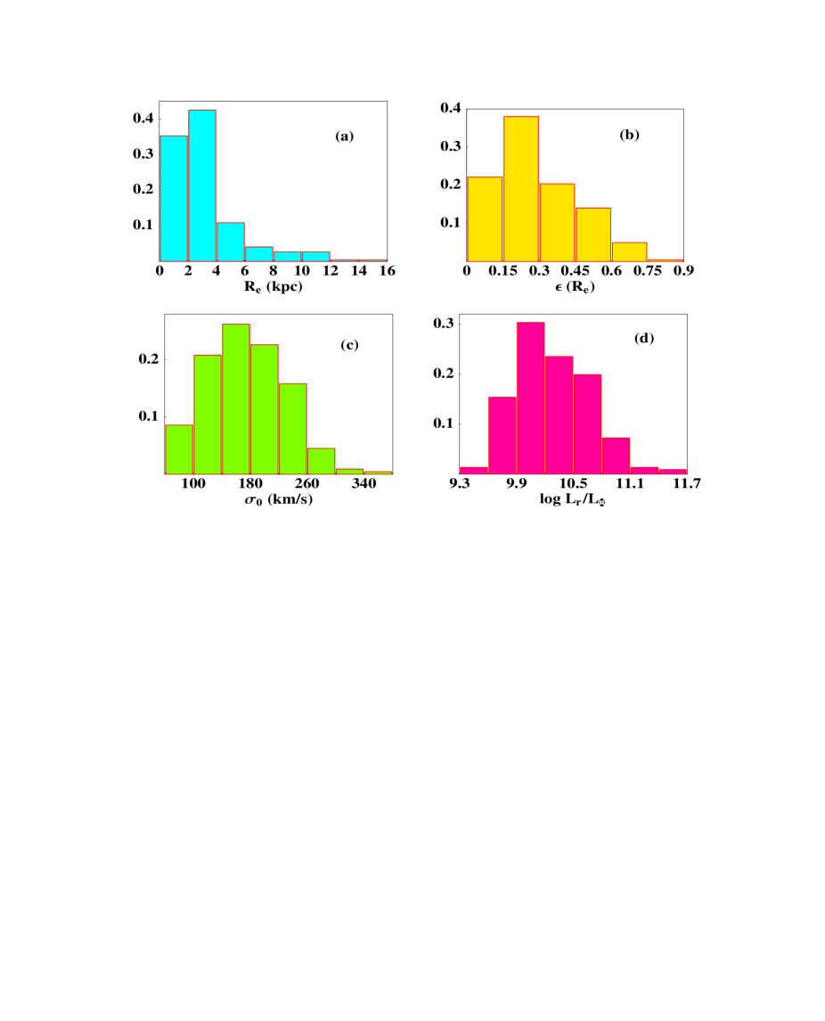
Figure 4: Histograms of sample galaxies properties: (a) effective radius $R_{e}$, (b) ellipticity $\epsilon$ at $R_{e}$, (c) central velocity dispersion $\sigma_{0}$ and (d) luminosity $L_{r}$ in Gunn–$r$ band .

The physical interpretation of the Fundamental Plane assumes the virial theorem to be the main constraint to the structure of ellipticals. Assuming elliptical galaxies to be 1–component and homologous systems, the virial theorem and the existence of the FP imply a slow but systematic variation of the mass–to–light ratio $M/L$ with the luminosity, whose physical origin is debated. This homology also determines a quasi–linearity of the relations connecting the gravitational and kinematic scale parameters of the galaxies to the observables $\sigma_{0}$ and $R_{e}$ (see Prugniel and Simien, 1997). However, according to the properties of the second, dark, mass component, this property could be lost, in such a way that the gravitational and photometric scales are not anymore connected in a simple, log–linear way.

                  

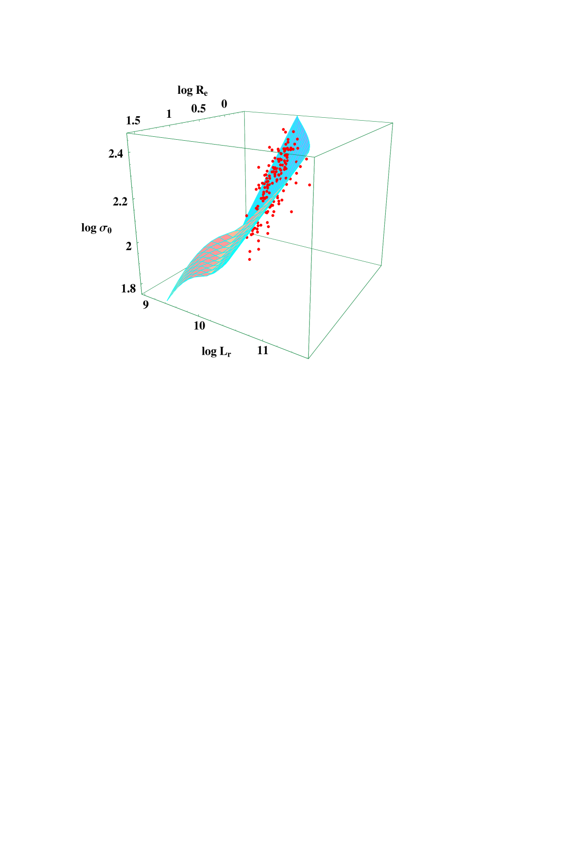
Figure 5: The surface in the log–space ($R_{e}$, $L_{r}$, $\sigma_{0}$) where we expect galaxies in the H+NFW scenario for $\Gamma_{vir}=30$, compared to sample data (red points). The units are: $R_{e}$ in kpc, $L_{r}$ in $L_{r\odot}$ and $\sigma_{0}$ in km/s.

We adjust the mass models parameters to fit the observations in the log–coordinates space: effective radius $R_{e}$, central velocity dispersion $\sigma_{0}\equiv\sigma_{A}(R_{e}/8)$ and total luminosity in Gunn–$r$ band, defined as $L=2\pi R_{e}^{2}I_{e}$. The effective surface brightness $I_{e}$ in L${}_{\odot}/$pc² is calculated from $\mu_{e}$ in mag arsec^-2: $\log I_{e}=-0.4\mu_{e}-26.4$, for Gunn–$r$ band (JFK, 1995a). In fitting the log–surface $\sigma_{0}(R_{e},\ L_{r})$ to the observations, we leave free the mass–to–light ratio $M_{sph}/L_{r}$ of the TBL component and, respectively, $\Gamma_{vir}$ in the H+NFW case and $\Gamma_{e}$ in the H+B case. In the latter, we assign a constant value to the parameter $r_{0}/R_{e}=2$, similar to results for spirals (Borriello and Salucci, 2001), as the fit depends very weakly on it. We characterize the mass–to–light ratio as $\Upsilon_{r}\equiv M_{sph}/L_{r}=\Upsilon_{r\ast}\ (L_{r}/L_{\ast})^{\alpha}$, with $\Upsilon_{r\ast}$ and $\alpha$ free parameters. Here, we neglect a possible weak dependence of $\Upsilon_{r}$ on $R_{e}$, but we will discuss this point later.

5.3 Results and discussion

5.3.1 H+NFW mass model

This model is unable to provide a plane surface in the log–space ($\sigma_{0}$, $R_{e}$, $L_{r}$), for plausible values of the free parameters. In Fig.5 we show the effect on the surface by adding to the stellar spheroid a dark NFW component with the reasonable dark–to–TBL mass ratio of $\Gamma_{vir}=30$. The surface curvature prevents us from properly fitting the data, especially in the region occupied by galaxies with large effective radius and low luminosity, for which the DM contribution to $\sigma_{0}$ is unacceptably high.

The results of the fitting procedure are shown in Fig.6, with contours representing $68\%$, $95\%$ and $99\%$ CL. The best–fit model is consistent with no DM at all ($\Gamma_{vir}=2\pm 4$ at 1 $\sigma$) and values of $\Gamma_{vir}\,\lower 2.0pt\hbox{${>\atop\hbox{\raise 4.0pt\hbox{$\sim$}}}$}\,10$ are excluded at $>95\%$ CL. Solutions very marginally permitted ($\Gamma_{vir}\simeq 10-15$) still require a very high efficiency of collapse of baryons in stars ($\sim 90\%$). This is at strong variance with the inferred budget of the cosmic baryons (Salucci and Persic, 1999) and with current ideas of galaxy formation, for which feedback mechanisms (such as SN explosions and central QSO activity) transfer thermal energy into the ISM and inhibit an efficient star formation (e.g. Dekel and Silk, 1986; Romano et al., 2002). They predict $\Gamma_{vir}$ to be significantly higher than the cosmological value of $\sim 8$.

     

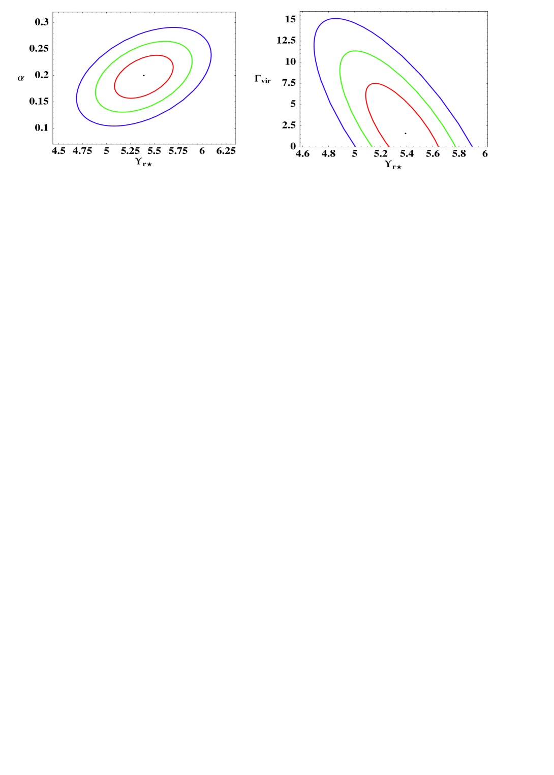
Figure 6: The mass model parameters, obtained by best–fitting the H+NFW surface in the log–space ($R_{e}$, $L_{r}$, $\sigma_{0}$) to the FP ($68\%$, $95\%$ and $99\%$ CL).

The mass–to–light ratio of the TBL component in Gunn–$r$ band is found $\sim 5$, i.e. well within values predicted by passive evolution of an old stellar population, generated with a standard IMF (e.g. Trager et al., 2000). As a matter of fact, this encourages us to consider the TBL mass as composed of just stellar populations.

The curvature of the surface in the logarithmic space of the observables is a consequence of the particular concentration–mass relation predicted by CDM N–body simulations. Anyway, once we assume a value for $\Gamma_{vir}$, we can consider different concentration parameters (for example, by moving a fraction of DM outside $R_{e}$). In order to illustrate the consequences, we have explored the realistic case of $\Gamma_{vir}=30$. For simplicity, we assume $c=c_{11}\cdot(M_{vir}/10^{11}M_{\odot})^{-0.13}$, and we look for values of $c_{11}$ for which CDM profiles are in agreement with the Fundamental Plane. In Fig.7 we show the value for $c_{11}$ implied by the narrowness of the observed FP. In order to have a small DM fraction inside $R_{e}$ and recover the FP, we must lower the concentration parameter down to $\sim 5$, well below the standard predictions of numerical simulations of halos in $\Lambda$CDM cosmology (e.g. Wechsler et al., 2002).

                                       

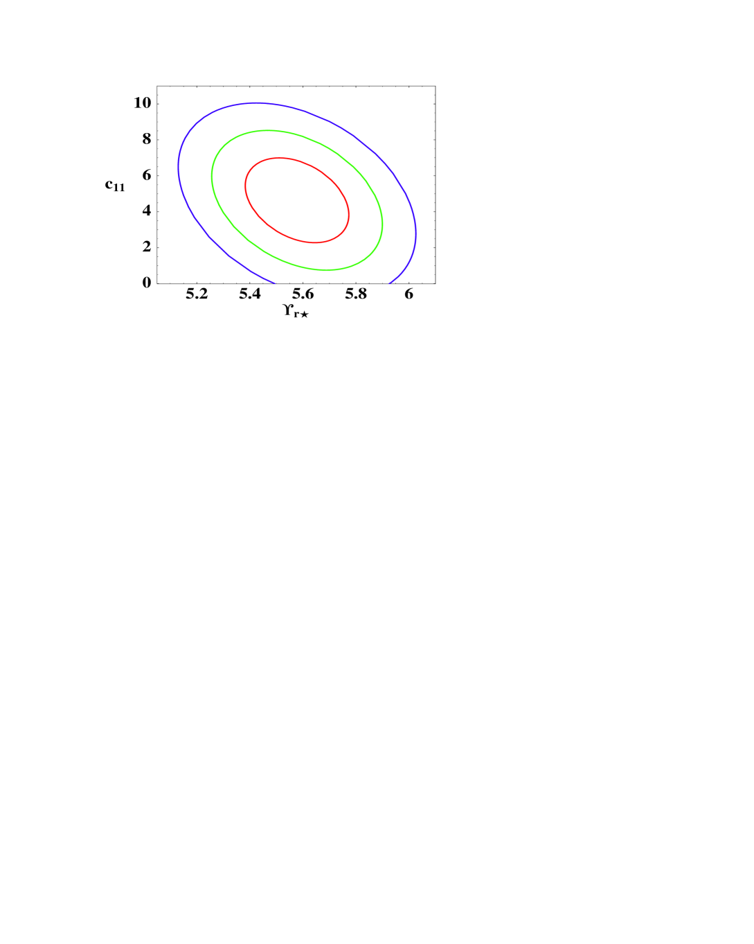
Figure 7: Concentration parameter $c_{11}$ and $\Upsilon_{r\ast}$ ($68\%$, $95\%$ and $99\%$ CL) in agreement with the observed FP, for H+NFW mass model with $\Gamma_{vir}=30$.

Again, it is worth noticing the robustness of the estimate of the mass–to–light ratio of the TBL component, which results to be insensitive to even such a model change.

5.3.2 H+B mass model

In this case, the presence of dark matter, distributed independently of the stellar profile, does not alter the FP surface shape, which still remains a plane. The best–fit mass model is obtained for (see Fig.8):

$$\Upsilon_{r}=(5.3\pm 0.1)\ \left(\frac{L_{r}}{L_{\ast}}\right)^{0.21\pm 0.03}$$ (15)

$$\Gamma_{e}=0.29\pm 0.06$$ (16)

(at $68\%$ CL). In Fig.9 (left) we show the $68\%$, $95\%$ and $99\%$ confidence contours for the TBL mass–to–light ratio parameters $\Upsilon_{r\ast}$ and $\alpha$. In the fit, the parameter $\Gamma_{e}$ is somewhat correlated to $\Upsilon_{r\ast}$: the greater DM amount in the bulge region, the lower the mass–to–light ratio of the TBL mass component. In Fig.9 (right) we show this correlation, marking the $\Gamma_{e}$ range corresponding to $99\%$ CL in $\Upsilon_{r\ast}$. Notice that a variation of $\Gamma_{e}$ of a factor $\sim 5$ corresponds to a much smaller variation of $\Upsilon_{r\ast}$, giving prominence to the strong stability of the stellar mass–to–light ratio we deduce from fits.

Finally, to check the reliability of the fit against our assumption of spherical stellar distribution, we perform the model fit by considering only 133 galaxies with small ellipticity ($\epsilon<0.3$); the resulting best–fit parameters are consistent with those of the whole sample, with a difference in the mean values of about $\sim 5\%$.

                          

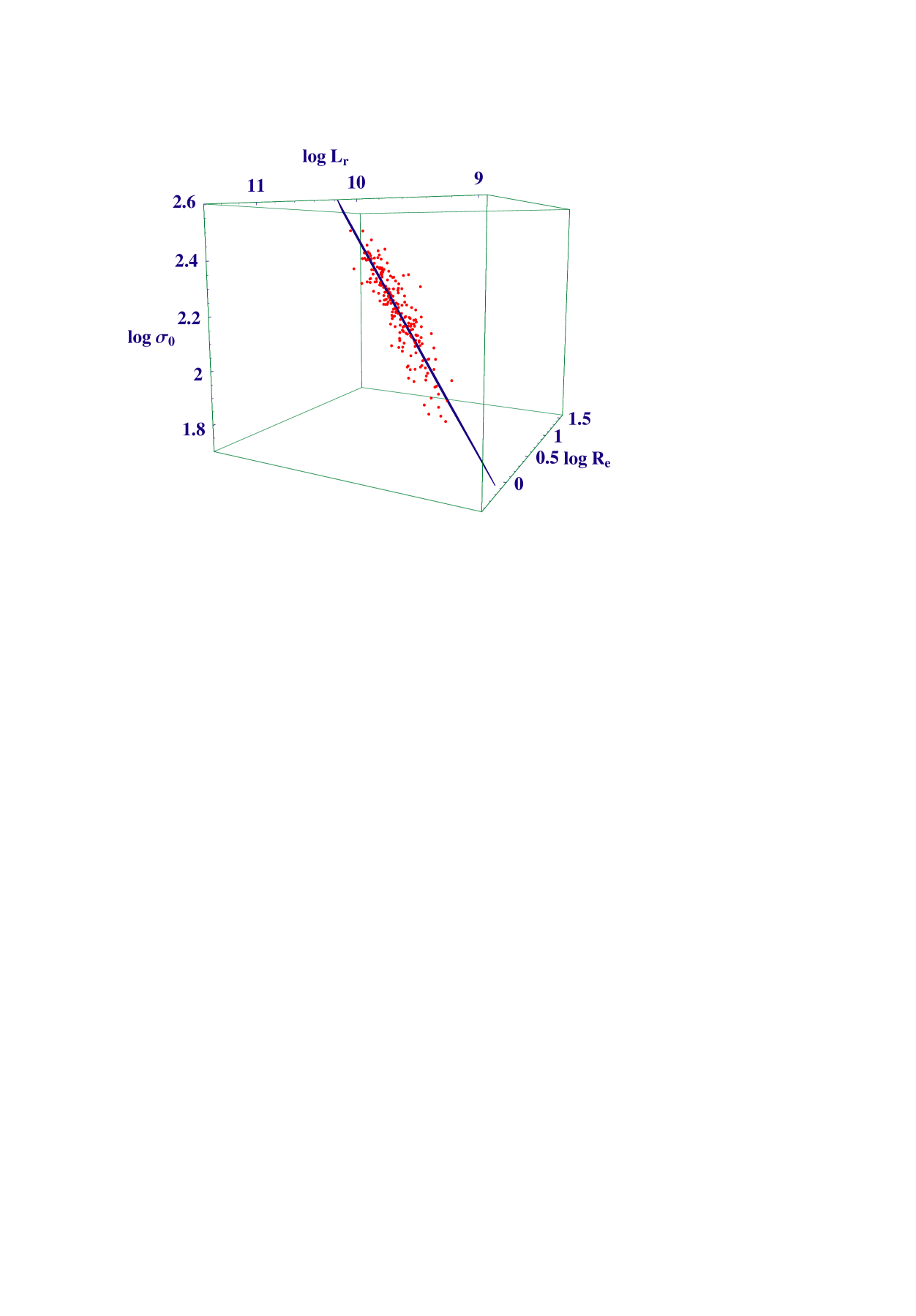
Figure 8: The H+B plane (edge–on), best fitting the data.

It is worth stressing that assuming $\Gamma_{e}$ constant in the fit is not the most general possibility and, in principle, the DM contribution within $R_{e}$ can well vary with luminosity. Although the investigation of this point is beyond the possibilities of our database, we notice that a variation would be in agreement even with recent dynamical and photometric studies of mass distribution in individual ellipticals (Kronawitter et al., 2000; Gerhard et al., 2001). Moreover, Gerhard et al. (2001) found $M_{DM}/M_{tot}|_{R_{e}}\sim 10-40\%$; in comparison we find $M_{DM}/M_{tot}|_{R_{e}}\sim 30\%$.

From eq.(14) we derive the relation between $\sigma_{0}^{2}R_{e}/G$ and the spheroid mass or, equivalently, the total mass within the effective radius $M_{e}\simeq(1+\Gamma_{e})\ 0.42\ M_{sph}$:

$$M_{sph}\ \simeq\ 5.4\ \frac{\sigma_{0}^{2}\ R_{e}}{G}$$ (17)

$$M_{e}\equiv M_{sph}(R_{e})+M_{h}(R_{e})\simeq\ 2.9\ \frac{\sigma_{0}^{2}\ R_{e}}{G},$$ (18)

using $F_{\rm B}=3.6\times 10^{-2}$ (see Fig.2) and the best–fit value $\Gamma_{e}=0.29$. Eq.(18) explicitly contains the effect of a DM halo and is to be compared with the “gravitational” mass at $R_{e}$ ($M_{G}\simeq 2\ \sigma_{0}^{2}\ R_{e}/G$), found by Burstein et al. (1997), taking the standard Keplerian formula $M_{e}=R_{e}V^{2}_{rot}/G$ and assuming $V^{2}_{rot}=3\sigma^{2}_{0}$. Eq.(17), instead, is in good agreement with results by Ciotti, Lanzoni and Renzini (1996); indeed they find for their HP model (a mass configuration similar to our H+B model) $M_{sph}=c_{M}\ \frac{\sigma_{0}^{2}\ R_{e}}{G}$ with $c_{M}\simeq 3-6$, according to the value of the total dark–to–TBL mass ratio (in the range $10-70$).

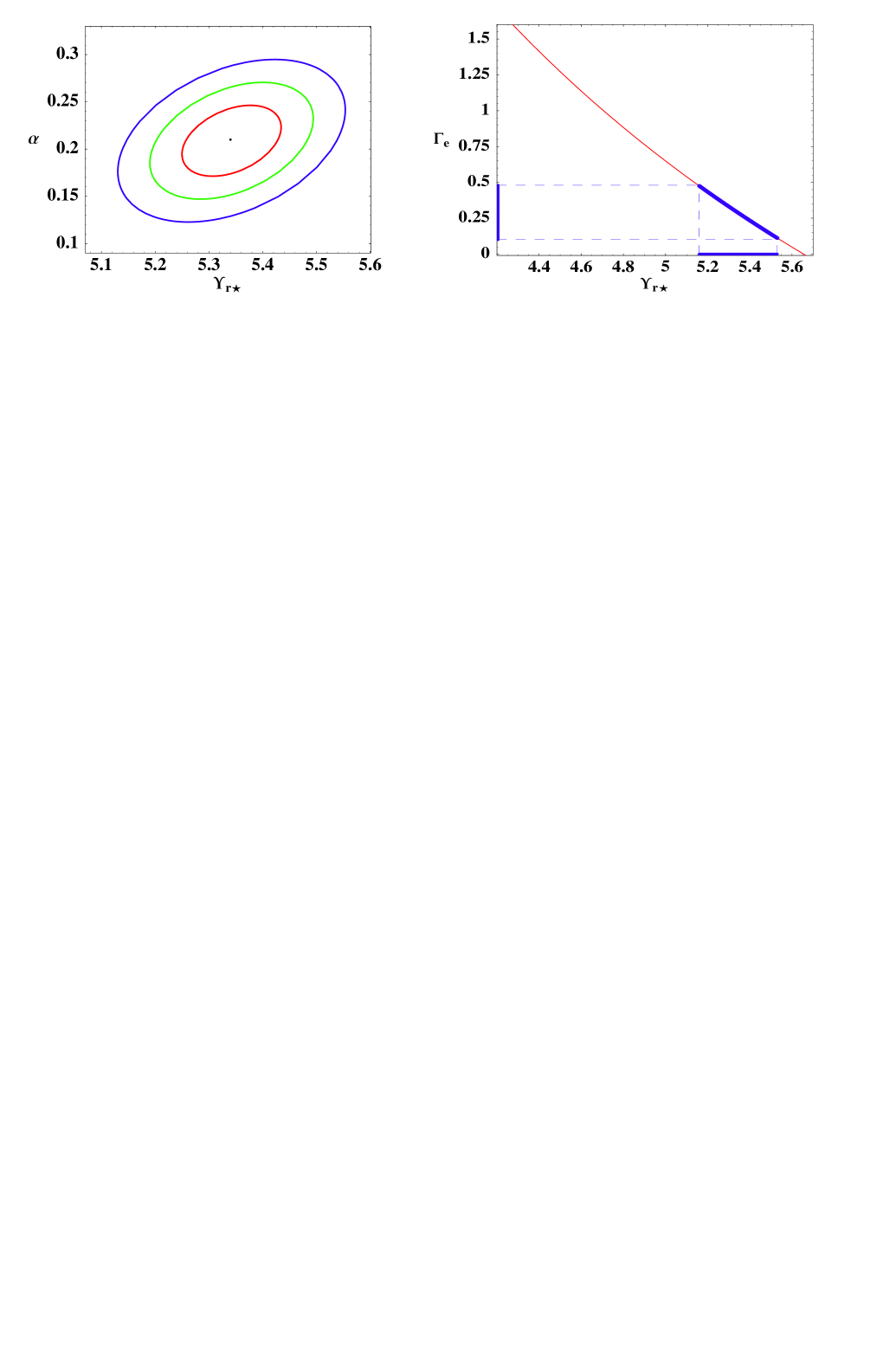
Figure 9: Best–fit H+B mass model: left) $68\%$, $95\%$ and $99\%$ CL for the stellar mass–to–light parameters; right) the correlation between $\Upsilon_{r\ast}$ and $\Gamma_{e}$, the dark–to–stellar mass ratio within $R_{e}$. Dashed lines mark the $99\%$ C.L. in $\Upsilon_{r\ast}$ and $\Gamma_{e}$.

In Fig.10 we show the distribution of the mass–to–light ratio in Gunn–$r$ band of the TBL component, obtained by inserting in eq.(17) the observed $\sigma_{0}$, $R_{e}$ and $L_{r}$. Continuous line is the mean correlation provided by the FP fit :

$$\Upsilon_{r}=5.3\ (L_{r}/L_{\ast})^{0.21}$$ (19)

By testing the residuals of the mass–to–light ratio as function of the effective radius $R_{e}$, we find no correlation within the statistical errors: $\Upsilon_{r}\propto R_{e}^{0.00\pm 0.05}$. A possible weak dependence on the effective radius, therefore, seems not sufficient to justify the scatter observed in the luminosity dependence of $M_{sph}/L$.

Since part of the galaxy sample has also been observed in different photometric bands (JFK, 1992; JFK, 1995a; see Tab.1), we investigated the $M_{sph}/L$ variations with luminosity (for a smaller number of galaxies) in Johnson $U$ and $B$ and Gunn–$v$ band, obtaining, respectively, the slopes $0.34\pm 0.05$, $0.27\pm 0.03$ and $0.25\pm 0.06$, with similar large scatter, thus independent of the photometric band. The slope of the relation $M_{sph}/L_{B}\propto L_{B}^{0.27\pm 0.03}$ seems to be smaller than the value of $\sim 0.6\pm 0.1$, obtained from velocity dispersion profiles analysis (Gerhard et al., 2001). Anyway, this slope tends to higher values when we consider a DM fraction (within $R_{e}$) decreasing with galaxy luminosity. For example, we obtain $M_{sph}/L_{B}\propto L_{B}^{0.45\pm 0.05}$ assuming $\Gamma_{e}=1$ for $L_{B}<10^{10}L_{\odot B}$ and $\Gamma_{e}=0.1$ for $L_{B}>10^{10}L_{\odot B}$.

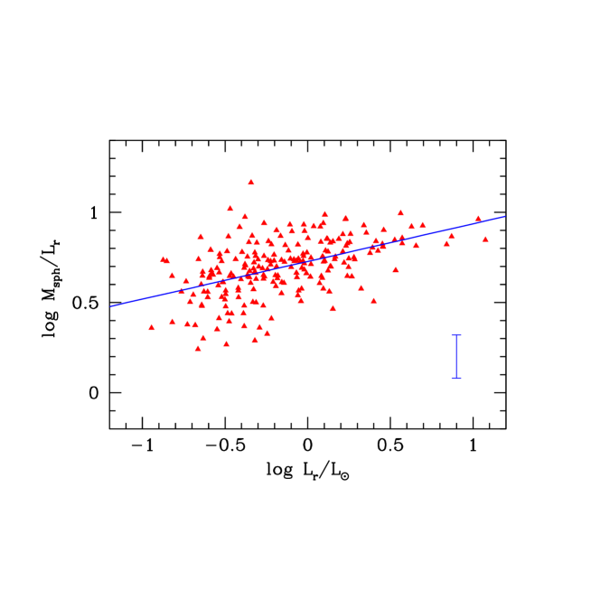
Figure 10: The distribution of the stellar mass–to–light ratio in Gunn–$r$ band. The continous line is the mean correlation provided by the FP fit. The typical data error at 1 $\sigma$ is also shown.

Recent observations have enlightened the potential of galaxy–galaxy (weak) lensing to probe the DM halo around galaxies at large radii, where it has been impossible, so far, to find kinematic tracers. Studies of weak lensing by SDSS collaborations (McKay et al., 2002; Guzik and Seljak, 2002) find $M_{260}/L_{r}\simeq 110$, for a $L_{r\ast}$ elliptical galaxy with a NFW dark matter halo ($M_{260}$ is the mass projected within an aperture of radius $260\ h^{-1}$ kpc). Since the first data bin is at $R=75\ h^{-1}$ kpc, the SDSS g–g lensing is not sensitive to small scales (where NFW and Burkert profiles actually differ); therefore, we can compare our results with SDSS ones. We estimate, at large radii, the dark–to–TBL mass ratio and the (total) mass–to–light ratio of the H+B mass model. In Fig.11 (left) we show the total (dark+TBL) mass–to–light ratio for a $L_{r\ast}$ elliptical galaxy. Assuming $R_{e}\simeq 5-10$ kpc for $L=L_{r\ast}$, the $260\ h^{-1}$ kpc aperture corresponds to $\sim(35-70)R_{e}$, for $h=0.7$. We obtain the value $M/L_{r}\simeq 110$ at this aperture for halo core radii in the range $\sim(2.4-2.8)\ R_{e}$. This value for the core is in agreement with the findings in spirals (Borriello and salucci, 2001) and suggests some form of DM–baryons interplay as the origin of the soft density cores in halos.

In Fig.11 (right) we show the cumulative dark–to–luminous mass ratio $M_{h}/M_{sph}$; the value we found above for the halo core radius of $r_{0}\simeq(2.4-2.8)R_{e}$ corresponds to a mass ratio, at very large radius, of $M_{h}/M_{sph}\simeq 15-30$. Remarkably, this range of values is in good agreement with results from spectro–photometric models of E’s formation in the spheroid mass range $3\times 10^{9}\,\lower 2.0pt\hbox{${<\atop\hbox{\raise 4.0pt\hbox{$\sim$}}}$}\,M_{sph}\,\lower 2.0pt\hbox{${<\atop\hbox{\raise 4.0pt\hbox{$\sim$}}}$}\,2\times 10^{11}$ (Romano et al., 2002; their Fig.10), models including even chimical evolution and feedback.

            

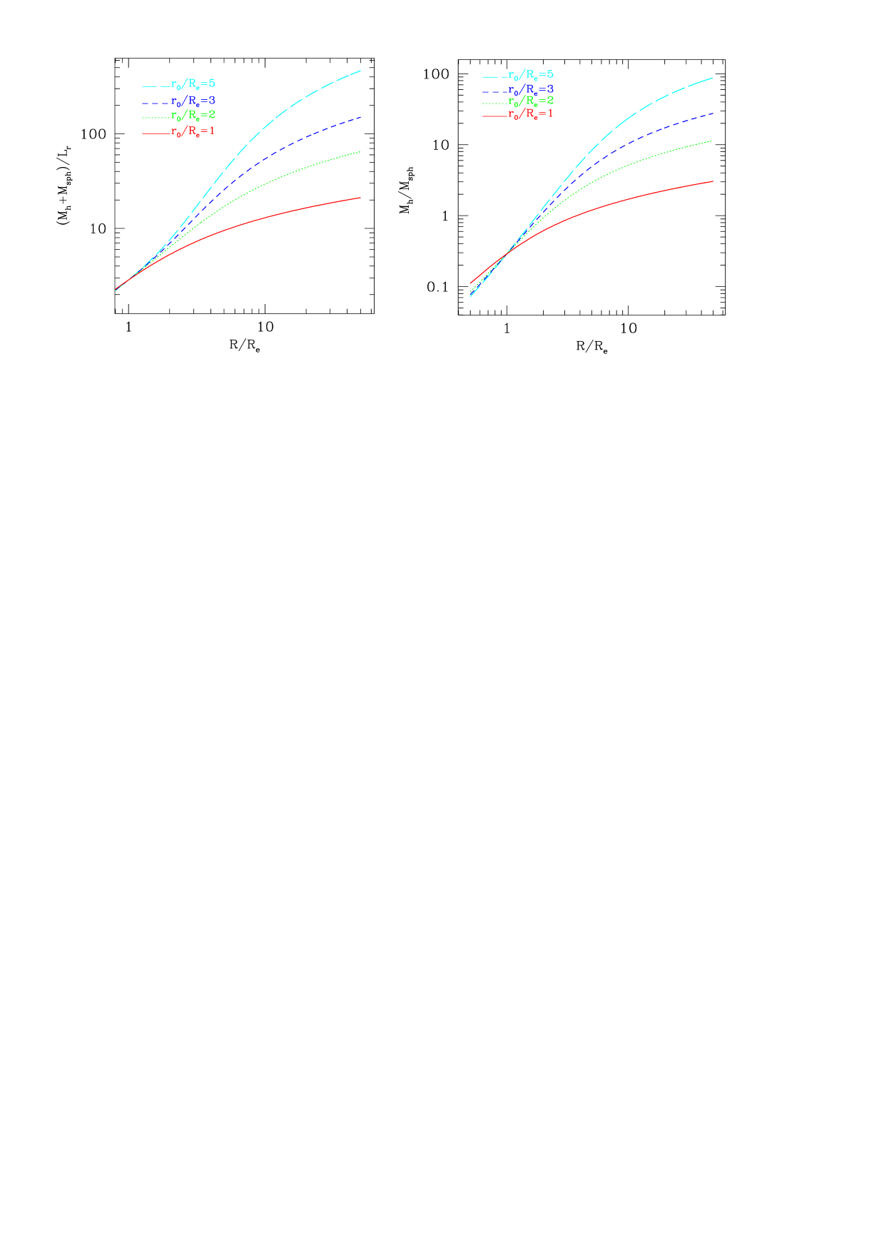
Figure 11: Properties of H+B mass model for a $L_{\ast}$ galaxy ($\Upsilon_{r}=5.3$, $\Gamma_{e}=0.3$): left) total (dark+TBL) mass–to–light ratio in Gunn–$r$ band vs. radius, for different values of halo core radius; right) dark–to–TBL mass ratio as function of the radius, for different values of $r_{0}/R_{e}$.

6 Summary and conclusions

We have shown that the very low scatter of elliptical galaxies around the Fundamental Plane can be statistically used to put very interesting constraints on DM distribution within them. The central velocity dispersion is the key quantity we have dealt with. We have briefly reviewed its relationship with the mass distribution of both traced–by–light and dark matter. Then, we selected a sample of 221 E/S0 galaxies with $L_{r}\geq 2\times 10^{9}$ $L_{\odot}$ in 9 clusters, endowed with very good photometric and spectroscopic data. The sample defines the classical FP in the log–space ($\sigma_{0}$, $R_{e}$, $L_{r}$), with the expected small scatter (0.084 in $\log\ R_{e}$, to be compared to a measurement uncertainty $\Delta\log R_{e}=\pm 0.045$).

We tested the reference model of cuspy DM distribution, namely the NFW model, and the cored model proposed by Burkert (1995). Our analysis shows that these luminous galaxies are largely dominated within the effective radius by matter traced by light, independently of the DM distribution model, cuspy or cored. In particular, for the cuspy NFW model, we have shown that the small scatter of our sample galaxies around the Fundamental Plane severely challenges the $\Lambda$CDM predictions. In such a theory, the structural properties of dark and luminous matter are so interwoven that in the log–space ($\sigma_{0}$, $R_{e}$, $L$) they produce a curved surface, rather than a plane, for plausible values of the total dark–to–TBL mass ratio. We conclude that in order to keep the small scatter around the FP we have either to keep $\Gamma_{vir}$ unacceptably low or to decrease the halo concentration well below the value currently predicted by simulations in $\Lambda$CDM cosmology.

Considering a cored DM density distribution, the agreement with the observed FP implies a dark–to–luminous mass fraction within the effective radius of $\sim 30\%$ and a luminosity dependence of the spheroid mass–to–light ratio in Gunn–$r$ band: $M_{sph}/L_{r}=(5.3\pm 0.1)(L_{r}/L_{\ast r})^{0.21\pm 0.03}$. An important result is the robustness of the mass–to–light ratio of the spheroidal component we obtained, which is in good agreement with predictions by stellar evolution models.

It is also worth noticing that, besides for spiral and dwarf galaxies, a cored DM halo, with low internal (within $2-3R_{e}$) density which increases as $r^{-3}$ at larger radii, is successful to explain also the structure of elliptical galaxies, pointing to an intriguing homogeneous scenario. Within this framework, we argue that dark matter in E’s can be investigated by a reasonably large number of galaxies with measures of l.o.s. velocity dispersion at $\sim R_{e}$. Although, so far, such observations have been severely hampered by the steep decreasing of the surface brigthness with radius, higher and higher sensitivity reached by recent surveys offers a good view to obtain a better resolution of the two mass components, in the whole region where baryons reside.

Acknowledgments

The authors would like to aknowledge financial support from ASI and from MIUR trough COFIN. We also thank the anonymous referee for very helpful comments.

Appendix A Velocity dispersion in detail

In this appendix, we will detail the procedure to compute velocity dispersions by means of Jeans hydrodynamic equations. Let us set all radii in units of the effective radius: $\tilde{r}\equiv r/R_{e}$, $\tilde{R}\equiv R/R_{e}$, $\tilde{r}_{0}\equiv r_{0}/R_{e}$, $\tilde{r}_{s}\equiv r_{s}/R_{e}$ and $\tilde{r}_{vir}\equiv r_{vir}/R_{e}$.

Mass distributions

Traced–by–light mass component - the radial profiles of mass density, mass and surface mass density are (Hernquist, 1990):

$$\rho_{sph}(\tilde{r})=\frac{k}{2\pi}\ \frac{M_{sph}}{R_{e}^{3}}\ F_{1}(\tilde{r})$$ (20)

$$M_{sph}(\tilde{r})=M_{sph}\ F_{2}(\tilde{r})$$ (21)

$$\Sigma(\tilde{R})=\frac{1}{2\pi\ k^{2}}\ \frac{M_{sph}}{R_{e}^{2}}\ F_{3}(\tilde{R})$$ (22)

where $k\simeq 0.5509$ and:

$$F_{1}(\tilde{r})=\frac{1}{\tilde{r}\ (\tilde{r}+k)^{3}}$$ (23)

$$F_{2}(\tilde{r})=\frac{\tilde{r}^{2}}{(\tilde{r}+k)^{2}}$$ (24)

$$F_{3}(\tilde{R})=\frac{\left[\left(2+\frac{\tilde{R}^{2}}{k^{2}}\right)X(\tilde{R})-3\right]}{(1-\frac{\tilde{R}^{2}}{k^{2}})^{2}}$$ (25)

with $X(\tilde{R})=[1-(\tilde{R}/k)^{2}]^{-1/2}{\rm Sech}^{-1}(\tilde{R}/k)$ for $0\leq\tilde{R}<k$
and

$X(\tilde{R})=[(\tilde{R}/k)^{2}-1]^{-1/2}{\rm Sec}^{-1}(\tilde{R}/k)$ for $\tilde{R}\geq k$.

Dark matter halo - the NFW mass profile reads:

$$M_{NFW}(\tilde{r})=M_{sph}\ \Gamma_{vir}\ \frac{A(\tilde{r},\tilde{r}_{s})}{A(\tilde{r}_{vir},\tilde{r}_{s})}$$ (26)

where, for any pair of variables $(x,y)$, $A(x,y)\equiv\ln(1+x/y)-x/(x+y)$. In particular, recalling that $c\equiv r_{vir}/r_{s}$, we have $A(\tilde{r}_{vir},\tilde{r}_{s})=\ln(1+c)-c/(1+c)$.

The Burkert halo mass profile is:

$$M_{B}(\tilde{r})=0.416\ M_{sph}\ \Gamma_{e}\ \frac{B(\tilde{r},\tilde{r}_{0})}{B(1,\tilde{r}_{0})}$$ (27)

where $B(x,y)\equiv-\arctan(x/y)+2\ln(1+x/y)+\ln[1+(x/y)^{2}]$.

By inserting eqs. (20), (21), (22), (26) and (27) in eqs. (2), (3) and (4) (after variables substitutions), we will obtain the velocity dispersions profiles:

Spheroid self–interaction terms

Out of the stellar spheroid self–interaction terms in velocity dispersions, $\sigma_{r;sph}^{2}$, $\sigma_{P;sph}^{2}$ and $\sigma_{A;sph}^{2}$, the first two can be analitically obtained (Hernquist, 1990):

$$\sigma_{r;sph}^{2}(\tilde{r})=\frac{1}{12\ k}\ \frac{GM_{sph}}{R_{e}}\ \left[\frac{12}{k^{4}}\ \tilde{r}\ (\tilde{r}+k)\ \ln\left(\frac{\tilde{r}+k}{\tilde{r}}\right)-\frac{\tilde{r}}{\tilde{r}+k}\cdot\right.$$

$$\left.\cdot\left(25+\frac{52}{k}\ \tilde{r}+\frac{42}{k^{2}}\ \tilde{r}^{2}+\frac{12}{k^{3}}\ \tilde{r}^{3}\right)\right]$$ (28)

$$\sigma_{P;sph}^{2}(\tilde{R})=\frac{1}{6\ k}\ \frac{GM_{sph}}{R_{e}}\ \frac{F_{4}(\tilde{R})}{F_{3}(\tilde{R})}$$ (29)

where:

$$F_{4}(\tilde{R})=\frac{1}{2}\ \left(1-\frac{\tilde{R}^{2}}{k^{2}}\right)^{-3}\left[-3\ \frac{\tilde{R}^{2}}{k^{2}}\ X(\tilde{R})\ \left(8\ \frac{\tilde{R}^{6}}{k^{6}}-28\ \frac{\tilde{R}^{4}}{k^{4}}+35\ \frac{\tilde{R}^{2}}{k^{2}}-20\right)+\right.$$

$$\left.-24\ \frac{\tilde{R}^{6}}{k^{6}}+68\ \frac{\tilde{R}^{4}}{k^{4}}-65\ \frac{\tilde{R}^{2}}{k^{2}}+6\right]-6\ \pi\ \frac{\tilde{R}}{k}$$ (30)

We obtain the luminosity weigthed velocity dispersion in the aperture $\tilde{R}_{A}\equiv R_{A}/R_{e}$, by integrating eq.(29):

$$\sigma_{A;sph}^{2}(\tilde{R}_{A})=\frac{1}{6\ k}\ \frac{GM_{sph}}{R_{e}}\ \frac{\int_{0}^{\tilde{R}_{A}}F_{4}(\tilde{R})\ \tilde{R}\ d\tilde{R}}{\int_{0}^{\tilde{R}_{A}}F_{3}(\tilde{R})\tilde{R}\ d\tilde{R}}$$ (31)

where integrals must be numerically performed. For the aperture $\tilde{R}_{a}=1/8$, we obtain the stellar contribution to the “central” velocity dispersion:

$$\sigma_{0;sph}^{2} = \frac{1}{6\ k}\ \frac{GM_{sph}}{R_{e}}\ \frac{\int_{0}^{1/8}F_{4}(\tilde{R})\ \tilde{R}\ d\tilde{R}}{\int_{0}^{1/8}F_{3}(\tilde{R})\ \tilde{R}\ d\tilde{R}}$$ (32)

$$\simeq 0.174\ \frac{GM_{sph}}{R_{e}}$$

Spheroid–halo interaction terms

We apply the same procedure for calculating the luminous–dark matter interaction terms: $\sigma_{r;h}^{2}$, $\sigma_{P;h}^{2}$ and $\sigma_{A;h}^{2}$. In this case, however, the integrations are always numerical.

H+NFW mass model:

$$\sigma_{r;NFW}^{2}(\tilde{r})=\frac{GM_{sph}}{R_{e}}\ \frac{\Gamma_{vir}}{A(\tilde{r}_{vir},\tilde{r}_{s})}\ \frac{\int_{\tilde{r}}^{\infty}\frac{F_{1}(\tilde{r}^{\prime})\ A(\tilde{r}^{\prime},\tilde{r}_{s})}{\tilde{r}^{\prime 2}}\ d\tilde{r}^{\prime}}{F_{1}(\tilde{r})}$$ (33)

$$\sigma_{P;NFW}^{2}(\tilde{R})=2\ k^{3}\ \frac{GM_{sph}}{R_{e}}\ \frac{\Gamma_{vir}}{A(\tilde{r}_{vir},\tilde{r}_{s})}\ \frac{\int_{\tilde{R}}^{\infty}\tilde{r}\ \frac{\int_{\tilde{r}}^{\infty}\frac{F_{1}(\tilde{r}^{\prime})\ A(\tilde{r}^{\prime},\tilde{r}_{s})}{\tilde{r}^{\prime 2}}\ d\tilde{r}^{\prime}}{\sqrt{\tilde{r}^{2}-\tilde{R}^{2}}}\ d\tilde{r}}{F_{3}(\tilde{R})}$$ (34)

$$\sigma_{A;NFW}^{2}(\tilde{R}_{A})=2\ k^{3}\ \frac{GM_{sph}}{R_{e}}\ \frac{\Gamma_{vir}}{A(\tilde{r}_{vir},\tilde{r}_{s})}\ \frac{\int_{0}^{\tilde{R}_{A}}\tilde{R}\ \frac{\int_{\tilde{R}}^{\infty}\tilde{r}\ \frac{\int_{\tilde{r}}^{\infty}\frac{F_{1}(\tilde{r}^{\prime})\ A(\tilde{r}^{\prime},\tilde{r}_{s})}{\tilde{r}^{\prime 2}}\ d\tilde{r}^{\prime}}{\sqrt{\tilde{r}^{2}-\tilde{R}^{2}}}\ d\tilde{r}}{F_{3}(\tilde{R})}\ d\tilde{R}}{\int_{0}^{\tilde{R}_{A}}F_{3}(\tilde{R})\ \tilde{R}\ d\tilde{R}}$$ (35)

where we can reduce the free parameters to the only virial mass i) by using eq.(9) for the virial radius, with $\Delta_{vir}(z=0)\simeq 337$:

$$r_{vir}\simeq 2.59\times 10^{-2}\left(\frac{M_{vir}}{M_{\odot}}\right)^{1/3}\ {\rm kpc}$$ (36)

and ii) by assuming $\Lambda$CDM $c-M_{vir}$ correlation (Wechsler et al., 2002, their Fig.16), which, together with eq.(36), gives:

$$r_{s}\equiv\frac{r_{vir}(M_{vir})}{c(M_{vir})}\simeq 6.17\left(\frac{M_{vir}}{10^{11}\ M_{\odot}}\right)^{0.48}\ {\rm kpc}$$ (37)

Burkert halo:

$$\sigma_{r;B}^{2}(\tilde{r})=0.416\ \frac{GM_{sph}}{R_{e}}\ \frac{\Gamma_{e}}{B(1,\tilde{r}_{0})}\ \frac{\int_{\tilde{r}}^{\infty}\frac{F_{1}(\tilde{r}^{\prime})\ B(\tilde{r}^{\prime},\tilde{r}_{0})}{\tilde{r}^{\prime 2}}\ d\tilde{r}^{\prime}}{F_{1}(\tilde{r})}$$ (38)

$$\sigma_{P;B}^{2}(\tilde{R})=0.831\ k^{3}\ \frac{GM_{sph}}{R_{e}}\ \frac{\Gamma_{e}}{B(1,\tilde{r}_{0})}\ \frac{\int_{\tilde{R}}^{\infty}\tilde{r}\ \frac{\int_{\tilde{r}}^{\infty}\frac{F_{1}(\tilde{r}^{\prime})\ B(\tilde{r}^{\prime},\tilde{r}_{0})}{\tilde{r}^{\prime 2}}\ d\tilde{r}^{\prime}}{\sqrt{\tilde{r}^{2}-\tilde{R}^{2}}}\ d\tilde{r}}{F_{3}(\tilde{R})}$$ (39)

$$\sigma_{A;B}^{2}(\tilde{R}_{A})=0.831\ k^{3}\ \frac{GM_{sph}}{R_{e}}\ \frac{\Gamma_{e}}{B(1,\tilde{r}_{0})}\ \frac{\int_{0}^{\tilde{R}_{A}}\tilde{R}\ \frac{\int_{\tilde{R}}^{\infty}\tilde{r}\ \frac{\int_{\tilde{r}}^{\infty}\frac{F_{1}(\tilde{r}^{\prime})\ B(\tilde{r}^{\prime},\tilde{r}_{0})}{\tilde{r}^{\prime 2}}\ d\tilde{r}^{\prime}}{\sqrt{\tilde{r}^{2}-\tilde{R}^{2}}}\ d\tilde{r}}{F_{3}(\tilde{R})}\ d\tilde{R}}{\int_{0}^{\tilde{R}_{A}}F_{3}(\tilde{R})\ \tilde{R}\ d\tilde{R}}$$ (40)

From eqs. (35) and (40), by setting $\tilde{R}_{a}=1/8$, we obtain the halos contributions to the central velocity dispersions given in eq.(13) and (14), where the functions $F_{NFW}$ and $F_{B}$ are defined as:

$$F_{NFW}\simeq 2\ \frac{k^{3}}{\int_{0}^{1/8}F_{3}(\tilde{R})\ \tilde{R}\ d\tilde{R}}\ \frac{1}{A(\tilde{r}_{vir}(M_{vir}),\tilde{r}_{s}(M_{vir}))}\ \cdot$$

$$\cdot\int_{0}^{1/8}\tilde{R}\ \frac{\int_{\tilde{R}}^{\infty}\tilde{r}\ \frac{\int_{\tilde{r}}^{\infty}\frac{F_{1}(\tilde{r}^{\prime})\ A(\tilde{r}^{\prime},\tilde{r}_{s}(M_{vir})}{\tilde{r}^{\prime 2}}\ d\tilde{r}^{\prime}}{\sqrt{\tilde{r}^{2}-\tilde{R}^{2}}}\ d\tilde{r}}{F_{3}(\tilde{R})}\ d\tilde{R}$$ (41)

$$F_{B}\simeq 0.83\ \frac{k^{3}}{\int_{0}^{1/8}F_{3}(\tilde{R})\ \tilde{R}\ d\tilde{R}}\ \frac{1}{B(1,\tilde{r}_{0})}\ \int_{0}^{1/8}\tilde{R}\ \frac{\int_{\tilde{R}}^{\infty}\tilde{r}\ \frac{\int_{\tilde{r}}^{\infty}\frac{F_{1}(\tilde{r}^{\prime})\ B(\tilde{r}^{\prime},\tilde{r}_{0})}{\tilde{r}^{\prime 2}}\ d\tilde{r}^{\prime}}{\sqrt{\tilde{r}^{2}-\tilde{R}^{2}}}\ d\tilde{r}}{F_{3}(\tilde{R})}d\tilde{R}$$ (42)

with the constant of proportionality: $k^{3}/\int_{0}^{1/8}F_{3}(\tilde{R})\ \tilde{R}\ d\tilde{R}\simeq 8.31$. Let us notice that $F_{NFW}$ depends on both $R_{e}$ and $M_{vir}\equiv\Gamma_{vir}\cdot M_{sph}$, while $F_{B}$ is only function of the parameter $\tilde{r}_{0}\equiv r_{0}/R_{e}$.

References

- [] Bertin, G., Bertola, F., Buson, L.M., et al., 1994, A&A, 292, 381
- [] Binney, J., Tremaine, S., 1987, Galactic Dynamics. Princeton Univ. Press, Princeton
- [] Blanton, M.R. et al. (2001) AJ, 121, 2358
- [] Borriello, A., Salucci, P., 2001, MNRAS, 323, 285
- [] Bryan, G.L., Norman, M.L., 1998, ApJ, 495, 80
- [] Bullock, J.S., Kolatt, T.S., Sigad, Y., Somerville, R.S., Kravtsov, A.V., Klypin, A.A., Primack, J.R., Dekel, A., 2001, MNRAS, 321, 559
- [] Burkert, A., 1995, ApJ, 447, L25
- [] Burstein, D., Bender, R., Faber, S.M., Nolthenius, R., 1997, AJ, 114, 1365
- [] Cheng, L., Wu, X., 2001, A&A, 372, 381
- [] Ciotti, L., 1999, ApJ, 520, 574
- [] Ciotti, L., Lanzoni, B., Renzini, A., 1996, MNRAS, 282, 1
- [] Cole, S., Lacey, C., 1996, MNRAS, 281, 716
- [] de Battista, V.P., Sellwood, J.A., 1998, ApJ, 493, L5
- [] de Block, W.J.G., McGaugh, S.S., Rubin, V.C., 2001, AJ, 122, 2396
- [] de Vaucouleurs, G., 1948, Ann. d’Astroph., 11, 247
- [] Dekel, A., Silk, J., 1986, ApJ, 303, 39
- [] Djorgovski, S., Davis, M., 1987, ApJ, 313, 59
- [] Dressler, A., Lynden-Bell, D., Burstein, D., Davies, R.L., Faber, S.M., Terlevich, R.J., Wegner, G., 1987, ApJ, 313, 42
- [] Flores, R.A., Primack, J.R., 1994, ApJ, 427, 1
- [] Fukushige, T., Makino, J., 1997, ApJ, 477, L9
- [] Gerhard, O.E., Kronawitter, A., Saglia, R.P., Bender, R., 2001, AJ, 121, 1936
- [] Ghigna, S., Moore, B., Governato, F., Lake, G., Quinn, T., Stadel, J., 2000, ApJ, 544, 616
- [] Guzik, J., Seljak, U., 2002, MNRAS, 335, 311
- [] Hernquist, L., 1990, ApJ, 356, 359
- [] Jørgensen, I., Franx, M., Kjaergaard, P., 1992, A&AS, 95, 489
- [] Jørgensen, I., Franx, M., Kjaergaard, P., 1995a, MNRAS, 273, 1097
- [] Jørgensen, I., Franx, M., Kjaergaard, P., 1995b, MNRAS, 276, 1341
- [] Jørgensen, I., Franx, M., Kjaergaard, P.,1996, MNRAS, 280, 167
- [] Koopmans, L.V.E., Treu, T., 2002, in press, astro-ph/0205281
- [] Kronawitter, A., Saglia, R.P., Gerhard, O.E., Bender, R., 2000, A&AS, 144, 53
- [] Loewenstein, M., White, R.E. III, 1999, ApJ, 518,50
- [] Matthias, M., Gerhard, O.E., 1999, MNRAS, 310, 879
- [] McKay, T.A. et al., 2002, ApJ submitted, astro-ph/0108013
- [] Moore, B., 1994, Nature, 370, 629
- [] Moore, B., Governato, F., Quinn, T., Stadel, J., Lake, G., 1998, ApJ, 499, L5
- [] Navarro, J.F., Frenk, C.S., White, S.D.M., 1997, ApJ, 490, 493
- [] Persic, M., Salucci, P., 1997, Dark and Visible Matter in Galaxies, in ASP Conf. Ser., 117, ed. Persic & Salucci
- [] Prugniel, Ph., Simien, S., 1997, A&A, 321, 111
- [] Romano, D., Silva, L., Matteucci, F., Danese, L., 2002, MNRAS in press, astro-ph/0203506
- [] Saglia, R.P., Bertin, G., Stiavelli, M., 1992, ApJ, 384, 433
- [] Saglia, R.P., Bertin, G., Bertola, F., et al., 1993, ApJ, 403, 567
- [] Salucci, P., Burkert, M., 2000, ApJ, 537, 9
- [] Salucci, P., Persic, M., 1999, MNRAS, 309, 923
- [] Trager, S.C., Faber, S.M., Worthey, G., Gonzalez, J.J., 2000, AJ, 120, 165
- [] van der Marel, R.P., 1991, MNRAS, 253, 710
- [] Wechsler, R.H., Bullock, J.S., Primack, J.R., Kravtsov, A.V., Dekel, A., 2002, ApJ, 568, 52
- [] White, S.D.M., Rees, M., 1978, MNRAS, 325, 1017