Spectroscopy of the neighboring massive clusters Abell 222 and Abell 223

We present a spectroscopic catalog of the neighboring massive clusters Abell~222 and Abell~223. The catalog contains the positions, redshifts, $R$ magnitudes, $V-R$ color, as well as the equivalent widths for a number of lines for 183 galaxies, 153 of them belonging to the A 222 and A 223 system. We determine the heliocentric redshifts to be $z=0.2126\pm 0.0008$ for A 222 and $z=0.2079\pm 0.0008$ for A 223. The velocity dispersions of both clusters in the cluster restframe are about the same: $\sigma=1014\hskip 1.00006pt\hbox to0.0pt{\raisebox{4.30554pt}{${+90}$}\hss}\raisebox{-1.50696pt}{${-71}$}\hskip 0.50003pt$  km s^-1 and $\sigma=1032\hskip 1.00006pt\hbox to0.0pt{\raisebox{4.30554pt}{${+99}$}\hss}\raisebox{-1.50696pt}{${-76}$}\hskip 0.50003pt$  km s^-1 for A 222 and A 223, respectively. While we find evidence for substructure in the spatial distribution of A 223, no kinematic substructure can be detected. From the red cluster sequence identified in a color–magnitude–diagram we determine the luminosity of both clusters and derive mass–to–light ratios in the $R$–band of $(M/L)_{\mathrm{A222}}=(202\pm 43)\leavevmode\nobreak\ h_{70}\leavevmode\nobreak\ M_{\sun}/L_{\sun}$ and $(M/L)_{\mathrm{A223}}=(149\pm 33)\leavevmode\nobreak\ h_{70}\leavevmode\nobreak\ M_{\sun}/L_{\sun}$. Additionally we identify a group of background galaxies at $z\sim 0.242$.

1 Introduction

A 222/223 are two Abell clusters at $z\approx 0.21$ separated by $\sim 14\arcmin$ on the sky, or $\sim 2600h_{70}^{-1}$ kpc, belonging to the Butcher et al. (1983) photometric sample. Both clusters are rich having Abell richness class 3 (Abell 1958). While these are optically selected clusters, they have been observed by ROSAT (Wang & Ulmer 1997; David et al. 1999) and are confirmed to be massive clusters. 9 spectra of galaxies in the cluster region, most of them being cluster members, were known (Sandage et al. 1976; Newberry et al. 1988) before Proust et al. (2000, hereafter PEL) published a list of 53 spectra and did a first kinematical study of this system. PEL also found 4 galaxies at the cluster redshift in the region between the clusters (hereafter “intercluster region”), indicating a possible connection between the clusters.

We report 184 independent redshifts for 183 galaxies in the field of Abell 222 and Abell 223, more than three times the number of redshifts previously known, as well as equivalent widths for a number of lines.

The paper is organized as follows. In Sect. 2 we describe the reduction of the spectroscopic and photometric data and discuss deviations from previous values in the literature. The spatial distribution and the kinematics of the double cluster system are examined in Sect. 3 with an emphasis on finding possible substructure. We determine the luminosity and mass–to-light ratio of the clusters by selecting the red cluster sequence in Sect. 4. Our results are summarized in Sect. 5. Throughout this paper we assume an $\Omega_{\Lambda}=0.7,\;\Omega_{\mathrm{m}}=0.3,\;H_{0}=70\leavevmode\nobreak\ h_{70}$ km s^-1 Mpc^-1 cosmology.

2 Data and Data Reduction

Multi-object spectroscopy of the two clusters Abell 222 and Abell 223 was performed at the NTT on three consecutive nights in December 1999. These nights were clear with occasional high cirrus. The instrument used was EMMI with grism 2, which has a resolution of 580 at 600 nm and a dispersion of 11.6 nm/mm. With the 2048x2048 CCD pixels of 24 $\mu$m this leads to a dispersion of 0.28 nm/pixel. With one exception two exposures of 2700 seconds each were taken for 6 fields, 3 on each cluster. For the field centered on A 222 in the second night only one exposure of 2700 seconds was available. The wavelength calibration was done using Helium–Argon lamps, which provided typically 20 lines used in the calibration. The calibration frames were taken at the beginning of the night for the masks used during that night, before the science exposures were made.

2.1 Reduction of spectroscopic data

For the data reduction a semi-automated IRAF package was written by the authors that cuts out the single spectra of the CCD frames and then processes these spectra using standard IRAF routines for single slit spectroscopy. The sky spectrum was removed from all spectra using a linear fit with a $2\sigma$ rejection on measurements on each side of the galaxy spectrum where the position of the galaxy on the slit permitted it. Measurements from only one side of the spectrum were used otherwise. A $2\sigma$ rejection was used to remove cosmic rays and hot pixels. Remaining hot pixels or cosmic rays in the sky spectrum introduced fake absorption features, while hot pixels or cosmic rays in the spectrum itself lead to fake emission features. These were removed by hand.

Because the sky spectrum removal was done column by column and no distortion correction was applied, some residual sky lines remained in the final spectra, most notably of the strong [O i] emission at 5577 Å. At the typical redshift of the cluster members of $z\approx 0.21$ this line does not coincide with any important feature and thus does not cause any problems in the subsequent analysis.

2.2 Redshift determination

The radial velocity determination was carried out using the cross-correlation method (Tonry & Davis 1979) implemented in the RVSAO package (Kurtz & Mink 1998). Spectra of late type stars and elliptical galaxies with known radial velocities were used as templates. The redshift determination was verified by visual inspection of identified absorption and emission features.

Figure 1: Comparison of redshift measurements for objects observed by us and with redshifts listed in PEL. The large panel shows the full sample, the inset is a blow up of the cluster region. The error bars are the internal errors reported by RVSAO.

The average internal error reported by RVSAO is $cz=68$ km s^-1. Adding this in quadrature to the estimated error of the wavelength calibration of $cz=110$ km s^-1, we estimate the error in the redshift determination of single galaxies to be $\delta z=0.0004$.

Fig. 1 shows a comparison of our redshift measurements and the redshifts listed by PEL. The obvious outlier in the large panel is from the sample of Sandage et al. (1976). The inset shows a broad agreement between our results and the values of PEL. Ignoring the obvious outlier, the average difference between the measurements is $\left<z-z_{\mathrm{PEL}}\right>=(0.2\pm 1.1)\times 10^{-3}$. Student’s t-test rejects the null hypothesis of different sample means with same variance at higher than the 99% level for the 23 cluster galaxies we have in common with PEL. However, Student’s t-test confirms the hypothesis of different sample means with same variance at higher than the 99% level for all their and our cluster members, indicating that PEL observed a sub–sample with a significantly different mean value from the larger sample we describe here.

We ruled out the possibility that this discrepancy could have been caused by taking all calibration frames before the science exposures were taken. This could have introduced a shift of the zero point if the masks were not moved back to their original position for the science exposures. We confirmed that this is not the case by determining the radial velocity of the subtracted sky spectrum in the wavelength calibrated frames. We found that, if a zero point shift occurred, it must be smaller than 30 km s^-1, confirming the accuracy of our data.

2.3 Equivalent widths

We measured equivalent widths for the [O ii]$\lambda$3727, [O iii]$\lambda$5007 emission lines, and H$\beta$ and H$\alpha$ emission and absorption lines. The integration ranges for the features and the continuum were fixed by the values given in Table 1.

Table 1: Restframe wavelength ranges for equivalent widths measurement. All wavelengths are given in Å. The last column gives the continuum range that was used for estimating the signal–to–noise ratio.

Feature	$\lambda_{\mathrm{cent}}$	line	blue cont.	red cont.	SNR
$[{O\textsc{ii}}]$	3727	3713 - 3741	3653 - 3713	3741 - 3801	3560 - 3680
$[{O\textsc{iii}}]$	5007	4997 - 5017	4872 - 4932	5050 - 5120	4450 - 4750
H$\beta$	4861	4830 - 4890	4800 - 4830	4890 - 4920	4050 - 4250
H$\alpha$	6563	6556 - 6570	6400 - 6470	-	6300 - 6450

[O ii] and H$\alpha$ are important indicators of star formation rates (Kennicutt 1998). To accurately determine the equivalent widths and in particular estimate their significance level we follow the definition of equivalent widths given by Czoske et al. (2001):

$$W_{\lambda}=\sum_{i=1}^{N_{\mathrm{int}}}\frac{f_{i}}{\overline{f_{\mathrm{c}}}}\Delta\lambda-N_{\mathrm{int}}\Delta\lambda,$$ (1)

where $f_{i}$ is the flux in pixel $i$, $N_{\mathrm{int}}$ is the number of pixels in the integration range, $\overline{f_{\mathrm{c}}}$ is the continuum level estimated as the mean of the continuum regions on either side of the line, and $\Delta\lambda$ is the dispersion in Å/pixel. Note that with this definition emission lines have positive equivalent widths.

The significance of an equivalent width measurement is given by (Czoske et al. 2001)

$$\sigma^{2}_{W_{\lambda}}=$$ (2)

$$\left(\frac{S}{N}\right)^{-2}\left[\left(W_{\lambda}+N_{\mathrm{int}}\Delta\lambda\right)\Delta\lambda+\frac{\left(W_{\lambda}+N_{\mathrm{int}}\Delta\lambda\right)^{2}}{N_{\mathrm{c}}}\right],$$

where the signal to noise ratio $S/N=\overline{f_{\mathrm{c}}}/\sigma_{\mathrm{c}}$, and $\overline{f_{\mathrm{c}}}$ is obtained by averaging over $N_{\mathrm{c}}$ pixel in the wavelength range given in Table 1.

All wavelengths are given in the restframe of the object. All spectra were normalized to a continuum fit before equivalent widths were measured. The catalog lists all [O ii] and [O iii] emission features and all H$\beta$ and H$\alpha$ emission and absorption features that were detected with a significance $>2\sigma$.

2.4 Photometry

Wide-field imaging of the cluster pair was performed over two nights in December 1999 with the Wide Field Imager on the ESO/MPG 2.2m on La Silla. Eleven 900 second exposures in $R$-band and three 900 second exposures in $V$ band were taken using a dithering pattern which filled the gaps between the CCDs in the mosaic in the coadded image. The image reduction was carried out using a combination of self–written routines and routines which are part of the IMCAT software package written by Nick Kaiser (http://www.ifa.hawaii.edu/$\sim$kaiser/imcat). The images were flattened with medianed night-sky flatfields from all the $R$ or $V$ band long exposure images taken over the two nights. The images were aligned using a process which assumes each CCD in the mosaic can be translated to a common detector–plane coordinate system using a linear transformation of coordinates (a shift in both axes and rotation allowed) and that the detector-plane coordinates can then be transformed into sky coordinates using a two dimensional polynomial, in this case a bi-cubic polynomial. The linear transformation from each CCD to the detector-plane is assumed to be constant for all the images whereas the transformation from detector-plane to sky coordinates is determined separately for each image to allow for both the pointing offsets in the dithering pattern and any changes in the distortion pattern between images. By comparing the positions of stars among the individual images and to the positions in the USNO catalog, both systems of equations for coordinate transformations were solved using $\chi^{2}$ minimization of the final stellar positions. The rms dispersion of the centroids of the stars used in the fitting were $0\aas@@fstack{\prime\prime}016$ among the input images and $0\aas@@fstack{\prime\prime}54$ between the input images and the USNO coordinates, with the average offset vector being consistent with zero in all regions of the image. Further details of this technique along with justifications for the linear translation between CCD and detector plane can be found in Clowe & Schneider (2001). The mapping of each input CCD was performed using a triangular method with linear interpolation which preserves surface brightness even if the mapping changes the area of a pixel. The resulting images were then averaged using a 3$\sigma$ clipping algorithm to remove cosmic rays and moving objects. The final $R$-band image can be found in Fig. 6.

Objects were detected in the $R$-band image using SExtractor (Bertin & Arnouts 1996), and the $V$-band magnitudes for the objects were measured using SExtractor in two-image mode. The FWHM of bright but unsaturated stars in the coadded images are $0\aas@@fstack{\prime\prime}87$ for $R$ and $1\aas@@fstack{\prime\prime}05$ in $V$. Zeropoints were measured from Landolt standard fields (Landolt 1992), but the $V$-band data is known to have been taken in non-photometric conditions. From isolating the red cluster galaxy sequence in a color-magnitude plot (Fig. 2), corrected for the $A_{B}=0.086$ mag dust extinction (Schlegel et al. 1998) using the conversion factors from Cardelli et al. (1989), and comparing to predicted colors of cluster elliptical galaxies in a passive evolution model (Fukugita et al. 1995), a correction of $-0.23$ mag has been applied to the $V$ magnitudes to correct for the additional atmospheric extinction. This correction also causes the stellar $V-R$ colors to have the theoretically expected values (Gunn & Stryker 1983).

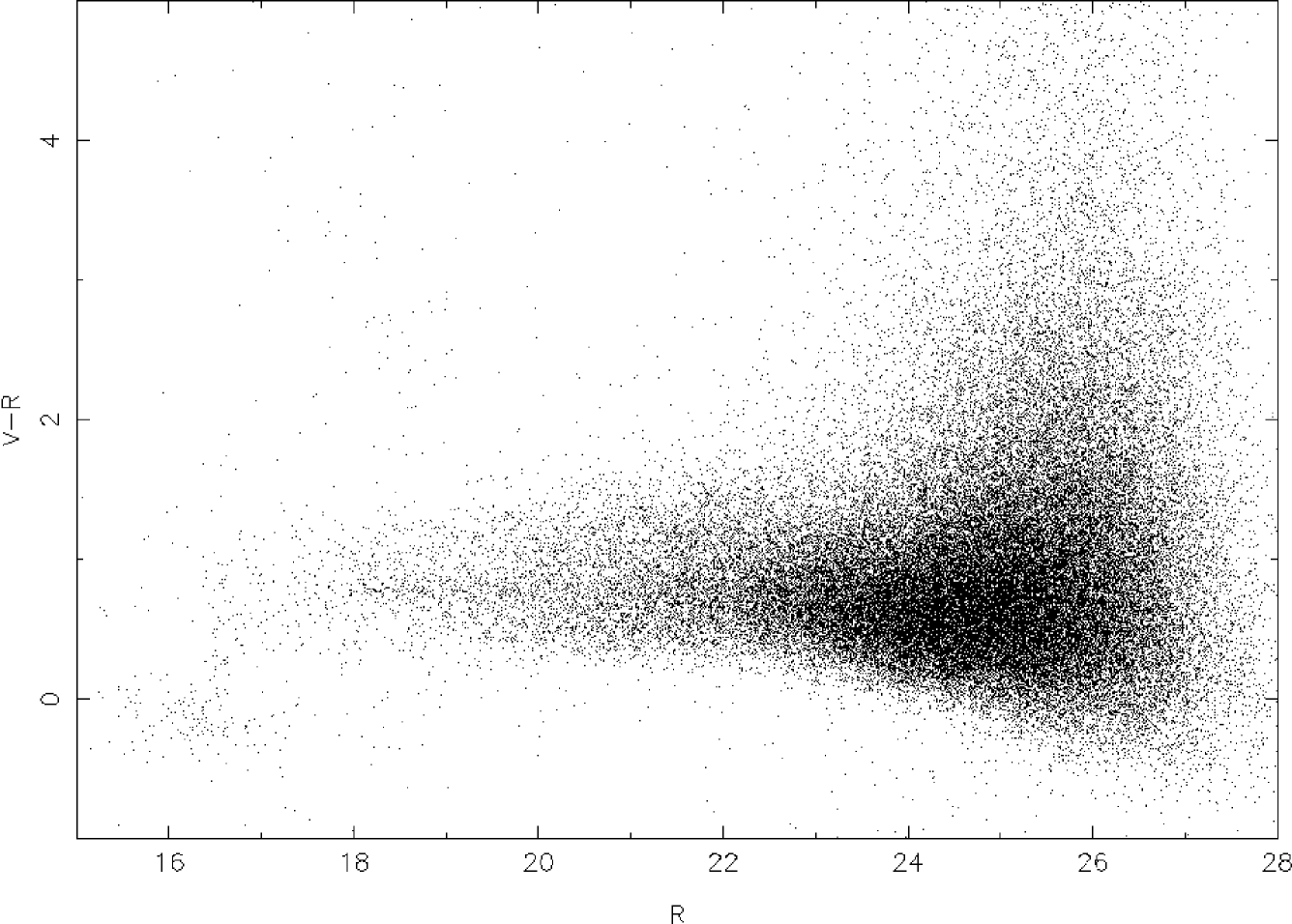
Figure 2: Color–magnitude plot with the already corrected $V$ magnitudes. The red cluster sequence is centered around $V-R=0.8$.

All magnitudes are isophotal magnitudes with the limiting isophote at 27.96 mag/$\mathrm{arcsec}^{2}$. We determine the completeness limit of the photometric catalog to be at $R=24$ mag from the point where the number counts of objects departs from a power law.

An excerpt from the big catalog of spectroscopically measured galaxies listing the 10 brightest galaxies in $R$–band in both cluster regions can be found in Table 2. The full catalog is available in electronic form at the at the Centre de Données astronomiques de Strasbourg (CDS).

Table 2: Excerpt from the full catalog listing the 10 brightest galaxies in $R$–band in both cluster regions. The column entries are 1. Object No. 2. right ascension (hour:minute:second) 3. declination (degree:minute:second) 4. $R$ band magnitude 5. $V-R$ color 6–9. observed equivalent widths of [O ii], [O iii], H$\beta$, and H$\alpha$ 10. & 11. heliocentric redshift and internal error reported by RVSAO 12. R-value of Tonry & Davis (1979) 13. notes, p: Proust et al. (2000), n: Newberry et al. (1988), s: Sandage et al. (1976), em: radial velocity derived from emission line template.

Object No.	RA (2000)	Dec (2000)	$R$	$V-R$	[O ii]/Å	[O iii]/Å	H$\beta$/Å	H$\alpha$/Å	$z_{\mathrm{hel}}$	$\sigma_{z_{\mathrm{hel}}}$	R	Notes
ABELL 222
93	01:37:41.54	$-$12:58:30.8	16.91	0.89	-	-	$-4.0\pm 1.6$	-	0.21318	0.00024	4.14
									0.21409	0.00022		p
30	01:37:26.34	$-$12:59:56.9	16.97	0.83	-	-	$-7.0\pm 1.4$	-	0.21347	0.00023	5.34
									0.21356	0.00007		p
65	01:37:34.01	$-$12:59:28.6	17.00	0.89	-	-	$-7.7\pm 1.6$	-	0.21329	0.00021	6.11
									0.21387	0.00012		p
8	01:37:17.97	$-$13:01:20.7	17.03	0.83	-	-	$-7.5\pm 1.7$	-	0.21132	0.00011	11.30
97	01:37:43.03	$-$12:57:43.7	17.41	0.84	-	-	$-6.7\pm 1.6$	-	0.21392	0.00026	4.86
									0.21371	0.00010		n
69	01:37:34.2	$-$12:56:52.7	17.44	1.01	-	-	$-6.8\pm 1.9$	-	0.20809	0.00028	4.05
16	01:37:22.65	$-$13:00:21.3	17.60	0.76	-	-	$4.9\pm 1.4$	-	0.21161	0.00019	6.13
13	01:37:21.21	$-$13:00:39.2	17.74	0.81	-	-	$-5.9\pm 1.3$	-	0.22067	0.00020	5.97
39	01:37:28.32	$-$12:55:55.7	17.77	0.66	-	$15.7\pm 0.5$	$9.3\pm 1.2$	$42.6\pm 0.7$	0.05147	0.00023	4.35	$0.05126\pm 0.00013$ measured on [O ii],
												[O iii], H$\beta$, H$\alpha$
95	01:37:42.08	$-$12:55:35.5	17.96	0.75	-	$1.9\pm 0.9$	$-3.4\pm 1.3$	-	0.21612	0.00019	5.87
…	…	…	…	…	…	…	…	…	…	…	…
ABELL 223
173	01:38:02.30	$-$12:45:19.5	16.58	0.83	$4.6\pm 1.9$	$3.2\pm 2.0$	$-3.5\pm 1.6$	-	0.20427	0.00025	4.55	$0.20459\pm 0.00009$ measured on[O iii],
												[N ii]
									0.20525	0.00013		p
									0.20506	0.00031		p
									0.20600	0.00167		s
186	01:38:04.83	$-$12:47:34.0	16.88	0.83	-	-	$-4.7\pm 2.1$	-	0.20972	0.00025	5.07
167	01:38:01.02	$-$12:46:51.6	17.00	0.79	-	-	$-4.6\pm 1.6$	-	0.21118	0.00024	5.14
140	01:37:56.02	$-$12:49:09.8	17.12	0.84	-	-	$-6.7\pm 1.9$	-	0.21050	0.00028	4.34
									0.21253	0.00030		p
172	01:38:02.19	$-$12:45:41.1	17.34	0.91	-	-	$-7.3\pm 1.7$	$-0.8\pm 0.3$	0.24074	0.00023	5.68
119	01:37:50.32	$-$12:46:15.4	17.36	0.75	-	-	$-3.5\pm 1.4$	-	0.20132	0.00018	6.66
193	01:38:07.25	$-$12:48:13.0	17.36	0.87	-	-	$-4.4\pm 1.5$	-	0.20957	0.00028	4.44
149	01:37:57.22	$-$12:50:17.1	17.40	0.68	$36.9\pm 3.4$	$15.8\pm 0.8$	-	$14.0\pm 2.4$	0.20707	0.00019	6.67	$0.20694\pm 0.00038$ measured on [O ii],
												[O iii], H$\beta$
									0.20839	0.00004		p
154	01:37:57.74	$-$12:47:55.8	17.41	0.83	-	-	$-7.7\pm 1.7$	-	0.21045	0.00025	4.82
									0.20971	0.00040		n
198	01:38:15.49	$-$12:43:38.4	17.48	0.80	-	-	$-5.2\pm 1.2$	$3.9\pm 0.9$	0.21560	0.00023	4.69
…	…	…	…	…	…	…	…	…	…	…	…

3 Spatial Distribution and Kinematics

After removing some obvious background and foreground galaxies ($z>0.3$ or $z<0.1$), an iterative $3\sigma$ clipping was used to decide upon cluster membership. We found 81 galaxies belonging to Abell 222 and 72 galaxies belonging to Abell 223 or the possible bridge connecting both clusters.

The mean redshift of the individual clusters are $z=0.2126\pm 0.0008$ and $z=0.2079\pm 0.0008$, for A 222 and A 223, respectively. This differs significantly from the values of $z=0.2143$ and $z=0.2108$ found by PEL for A 222 and A 223, respectively. The quoted errors include the statistical error of $\delta z=0.0005$ added linearly to the estimated error of the cluster member selection of $\delta z=0.0003$. This systematic error was estimated from varying the cut level of the recursive clipping procedure from $2\sigma$ to $3.5\sigma$ and calculating the means of these cuts. The statistical errors were calculated from a bootstrap resampling of the cluster members. The measured velocity dispersions have to be transformed to the restframe of the cluster according to the transformation law

$$\sigma_{\mathrm{cor}}=\frac{\sigma}{1+\overline{z}}\leavevmode\nobreak\ ,$$ (3)

(Harrison 1974). The restframe velocity dispersions for the individual clusters are $\sigma_{\mathrm{cor}}=1014\hskip 1.00006pt\hbox to0.0pt{\raisebox{4.30554pt}{${+90}$}\hss}\raisebox{-1.50696pt}{${-71}$}\hskip 0.50003pt$ km s^-1 and $\sigma_{\mathrm{cor}}=1032\hskip 1.00006pt\hbox to0.0pt{\raisebox{4.30554pt}{${+99}$}\hss}\raisebox{-1.50696pt}{${-76}$}\hskip 0.50003pt$ km s^-1, for A 222 and A 223, respectively. This is in good agreement with the values found by PEL of $\sigma=1013\pm 150$ km s^-1 and $\sigma=1058\pm 160$ km s^-1 for A 222 and A223, respectively. The errors of the velocity dispersion are the $(1-\alpha)=68\%$ confidence interval given by

$$\frac{(n-1)\sigma^{2}}{\chi^{2}_{n-1;\alpha/2}}<\sigma^{2}<\frac{(n-1)\sigma^{2}}{\chi^{2}_{n-1;1-\alpha/2}}\leavevmode\nobreak\ ,$$ (4)

for $n$ galaxies in the sample. The redshift and velocity dispersion for A 223 do not change significantly if the 3 galaxies from the intercluster region in our sample are removed. Figs. 3 to 5 show the corresponding radial velocity distributions of the individual samples.

Figure 3: Radial velocity distribution of all galaxies in the sample. The main peak corresponds to the two Abell clusters.

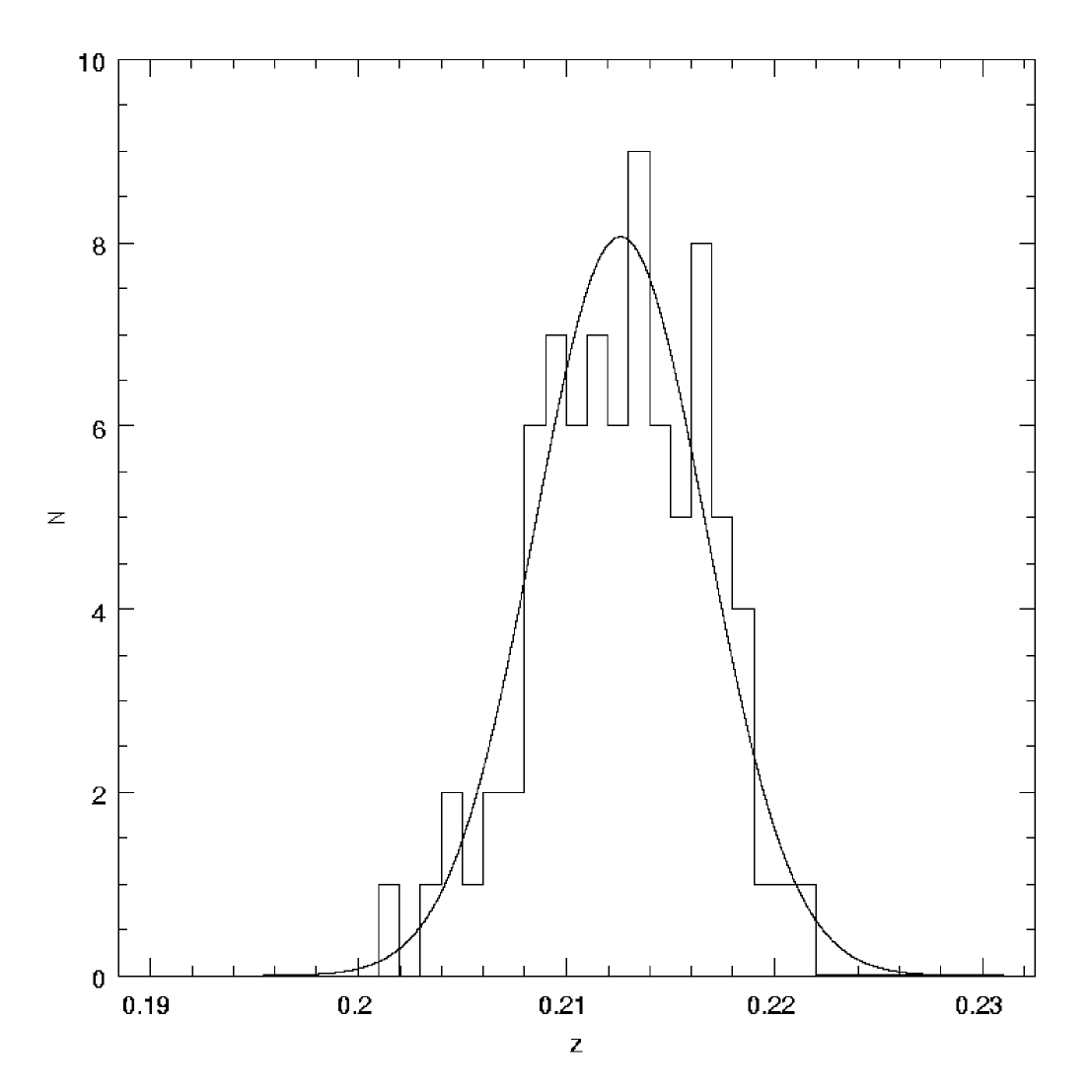
Figure 4: Radial velocity distribution of the members of A 222. The continuous line is a Gaussian with mean and measured dispersion value as given in the text.

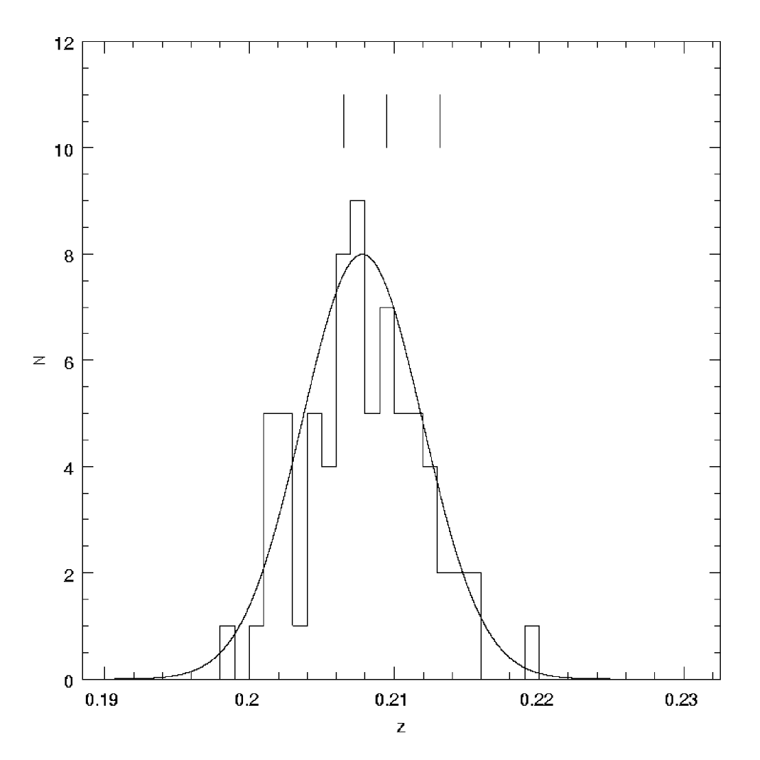
Figure 5: Same as Fig. 4 for A 223. The dashes denote the 3 galaxies in the bridge for which we measured radial velocities.

The values for the velocity dispersion are somewhat higher than those derived from X–ray luminosities. David et al. (1999) report bolometric luminosities of $L_{\mathrm{X}}=7.65\times 10^{44}$ erg s^-1 and $L_{\mathrm{X}}=6.94\times 10^{44}$ erg s^-1 from ROSAT PSPC observations for A 222 and A 223, respectively, for $H_{0}=50$ km s^-1 Mpc^-1. Using the $L_{\mathrm{X}}$–$\sigma$ relationships of Wu et al. (1999) we get $\sigma_{\mathrm{X}}=845-887$ km s^-1 for A 222 and $\sigma_{\mathrm{X}}=828-871$ km s^-1 for A 223. Compared to the velocity dispersions derived from the spectroscopic observations, both cluster appear to be underluminous in X–rays.

Together with the data of PEL we now have radial velocities for 6 galaxies in the possible bridge connecting both clusters. With our new values for the radial velocity of A 223 the observation made by PEL, that most of the bridge galaxies are in the low–velocity tail, does not hold anymore. In fact they all appear to be close to the maximum or higher of the velocity histogram shown in Fig. 5. Because A 222 is the cluster at higher redshift, this is the expected behavior should these galaxies indeed belong to a bridge connecting both clusters

SExtrator also provides an algorithm to separate galaxies from stars. Each object is assigned a CLASS_STAR value, which is 1 for stars, 0 for galaxies, and lies in between for ambiguous objects. Fig. 6 displays a projected galaxy number density map generated with the adaptive kernel density estimate method described by Pisani (1996) for a color selected sample of 702 objects with $R<21$ and $0.7<V-R<0.9$ and SExtractor CLASS_STAR $<0.1$ from the WFI images. Overplotted are the positions of all spectroscopically identified cluster members.

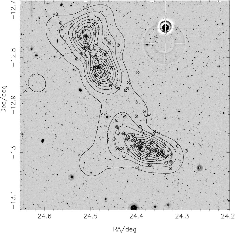
Figure 6: Deep $R$ band image of A 222 and A 223. The galaxy density contours are generated from a color selected sample of 702 objects. See text for details. The small circles mark all spectroscopically identified cluster galaxies.

Fig. 6 clearly exhibits two density peaks in A 223. Both peaks are separated by $4\aas@@fstack{\prime}8$ and are centered at ($\alpha$=01:37:53.5, $\delta$=$-$12:49:21.2) and ($\alpha$=01:38:01.8, $\delta$=$-$12:45:07.0). These peaks are also visible in the density distribution of the 181 spectroscopically identified cluster galaxies. Also visible is an overdensity of color selected objects in the intercluster region, hinting at a connection between both clusters.

We applied the Dressler & Shectman (1988, DS) test for local kinematic deviations in the projected galaxy distribution. The DS test is based on computing deviations of local mean velocity and velocity dispersion from the global values. The local values are calculated for each of the $N$ galaxies and its $n-1$ nearest neighbors. The statistics used to quantify the presence of substructure is

$$\Delta = \sum_{i=1}^{N}\delta_{i}$$ (5)

$$= \sum_{i=1}^{N}\left\{\frac{n}{\sigma_{\mathrm{glob}}^{2}}\left[\left(\overline{v}_{\mathrm{glob}}-\overline{v}_{\mathrm{loc,i}}\right)^{2}+\left(\sigma_{\mathrm{glob}}-\sigma_{\mathrm{loc,i}}\right)^{2}\right]\right\}^{\frac{1}{2}}$$

The $\Delta$ statistics is calibrated by randomly shuffling the radial velocities while keeping the observed galaxy positions fixed. The significance of the observed $\Delta_{\mathrm{obs}}$ is assessed by the fraction of simulations whose $\Delta_{\mathrm{sim}}$ is smaller than $\Delta_{\mathrm{obs}}$.

We find that, while the DS test is clearly able to separate both clusters at better than the 99.9% confidence level, it does not find any substructure in the individual clusters for values of $8<n<16$.

Also the DIP statistic (Hartigan & Hartigan 1985), which we calculated with the FORTRAN routine provided by Hartigan (1985), is not able to reject the null hypothesis of an unimodal distribution for any of the cluster samples. We tested for deviations from a normal Gaussian distribution by computing the skewness and kurtosis of both cluster samples. We found that we cannot reject a Gaussian parent population for both cluster samples at the $1\sigma$ level.

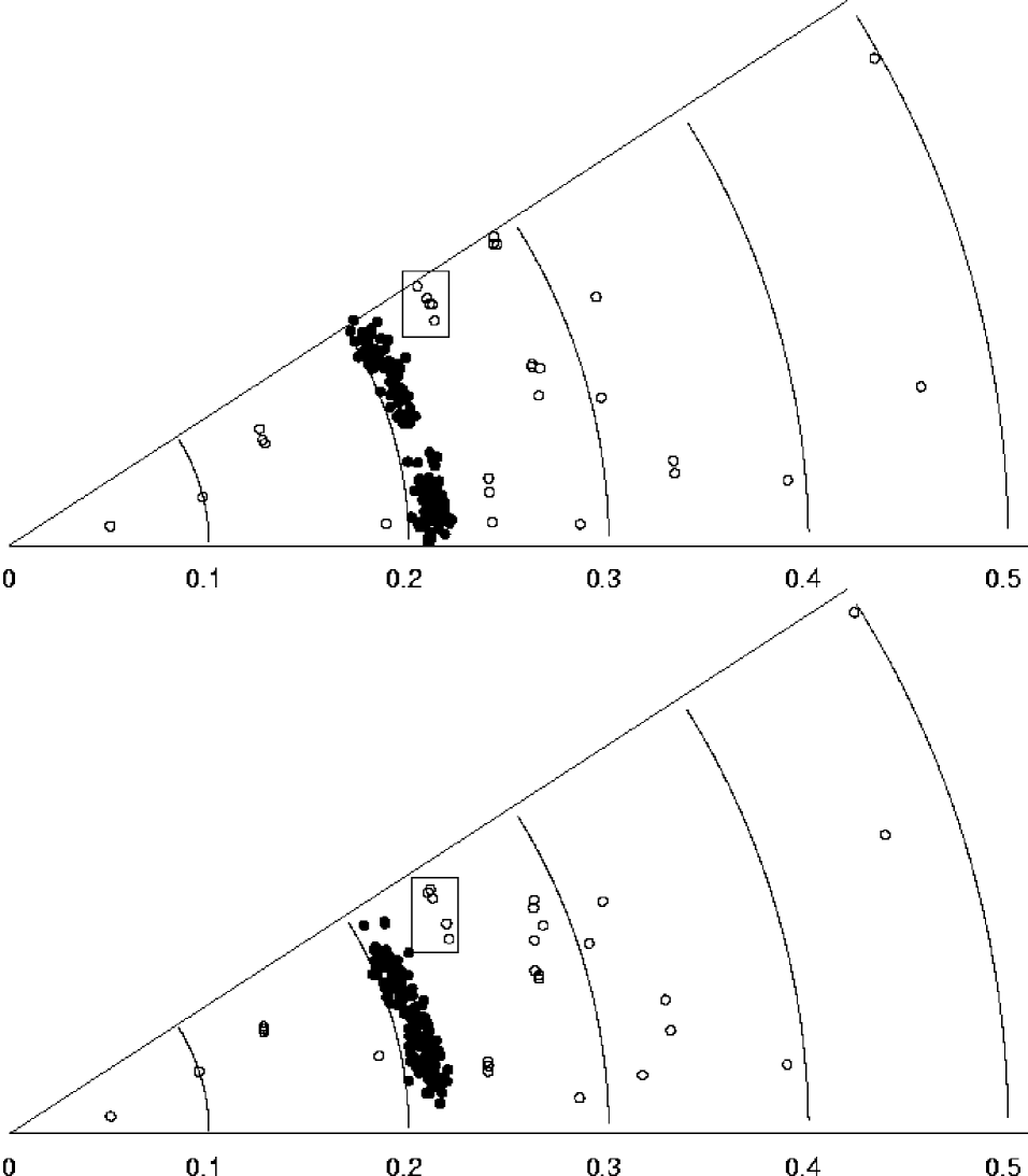
Figure 7: Declination (top) and right ascension (bottom) wedge redshift diagram. Cluster members are plotted as solid circles while background and foreground galaxies are displayed with open symbols. The rectangle highlights a small background group of galaxies. The opening angle is from $-$13°2′24″ to $-$12°16′24″ for the declination wedge and from 01:37:04.8 to 01:38:48.0 for the right ascension wedge.

The wedge velocity diagrams in Fig. 7 clearly show the Abell system at $z\sim 0.21$. A small group of five galaxies can be seen behind A 223 at $z=0.242$. We derive a velocity dispersion of $\sigma=330$ km s^-1, confirming that it is not only close in the projected spatial distribution but also in redshift space.

4 Mass–to–light ratio

To determine the luminosity of the clusters we applied the same cut on color and CLASS_STAR as above in a circle with 1.4 $h_{70}^{-1}$ Mpc radius around the bright cD galaxy of A 222 and the center of the line connecting both density peaks in A 223. We binned the selected objects in bins of 0.5 mag and fitted a Schechter (1976) luminosity function,

$$n(L)\mathrm{d}L=n^{*}(L/L^{*})^{\alpha}\exp(-L/L^{*})\mathrm{d}(L/L^{*})\leavevmode\nobreak\ ,$$ (6)

where $L^{*}$ is the characteristic luminosity, $\alpha$ is the faint–end slope, and $n^{*}$ is a normalization constant. Written in terms of absolute magnitude Eq. (6) becomes

$$N(M)\mathrm{d}M=kn^{*}\exp\left\{\left[-k(\alpha+1)(M-M^{*})\right]\right.$$

$$-\left.\exp\left[-k(M-M^{*})\right]\right\}\mathrm{d}M\leavevmode\nobreak\ ,$$ (7)

where $M^{*}$ is the absolute magnitude corresponding to $L^{*}$ and $k=\ln 10/2.5$ (Kashikawa et al. 1995). Using k correction and a passive evolution correction on the synthetic elliptical galaxy spectra of Bruzual & Charlot (1993), for the Abell system $M_{R}=m_{R}-5\log\left(\frac{d_{\mathrm{l}}}{\mathrm{Mpc}}\right)-24.91$, $d_{\mathrm{l}}$ being the luminosity distance.

The fit is performed by minimizing the quantity

$$\chi^{2}=\sum\frac{\left[N(M_{i})-N_{f}(M_{i})\right]^{2}}{\sigma_{i}^{2}}\leavevmode\nobreak\ ,$$ (8)

with $N(M_{i})$ and $N_{f}(M_{i})$ being the observed and fitted number of galaxies in the $i$th magnitude bin. The variance of galaxies in each magnitude bin was assumed to be that of a Poissonian distribution.

The best–fit Schechter function for A 222 has $M^{*}=-22.1\pm 0.2$, $\alpha=-1.04\pm 0.12$, and $n^{*}=31\pm 11$. The $\chi^{2}$ value for these parameters is 12.7 with 7 degrees of freedom. The best–fit parameters for A 223 are $M^{*}=-23.1\pm 0.2$, $\alpha=-1.20\pm 0.06$, and $n^{*}=15\pm 5$ with a minimum $\chi^{2}$ value of 7.0, also for 7 degrees of freedom. From Figs. 8 and 9 we see, that the Schechter function is a good representation of the faint end, while it slightly underpredicts the number of bright galaxies. Although the values of $M^{*}$ differ by one magnitude they are compatible with values from the literature. E.g. Trèvese et al. (1996) find $M^{*}=-22.66\pm 0.52$ from a study of 36 Abell clusters for a fixed $\alpha=-1.25$. For this value of $\alpha$ the $M^{*}$ value for A 222 increases to $-22.4$, but the fit then has a reduced $\chi^{2}$ of 2.2. In the following we only use the lower value of $M^{*}=-22.1$ for A 222.

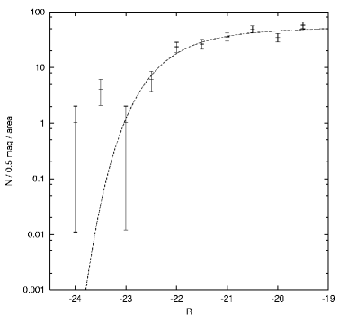
Figure 8: Differential $R$–band luminosity function for A 222. The points represent the objects selected by the criteria detailed in the text, while the dashed line is the best–fit Schechter function.

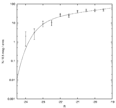
Figure 9: Same as Fig. 8 for A 223.

The total $R$–band luminosity of the red cluster sequence is determined by extrapolating the luminosity function. The observed fraction of the total luminosity is given by $\Gamma(\alpha+2,L_{\mathrm{lim}}/L^{*})/\Gamma(\alpha+2)$, where $\Gamma(\cdot,\cdot)$ is the incomplete Gamma function, $L_{\mathrm{lim}}$ is the completeness limit, which in this case is given by the selection parameters, and $L^{*}$ is the luminosity corresponding to the fitted $M^{*}$ (Tustin et al. 2001). It follows from the chosen magnitude cut and the size of the bins, that in our case the limiting magnitude $M_{R}=-19.0$. This implies that we observe $91.4\%$ and $81.7\%$ of the total light in A 222 and A 223, respectively. The total $R$–band luminosity of the red cluster sequence then is $L_{R}=(3.1\pm 0.3)\times 10^{12}\;h_{70}^{-2}\;L_{\sun}$ for A 222 and $L_{R}=(4.4\pm 0.4)\times 10^{12}\;h_{70}^{-2}\;L_{\sun}$ for A 223, where the errors reflect the uncertainty in the parameters of the luminosity function.

We compute mass–to–light ratios assuming an isothermal sphere model for both clusters with the velocity dispersion determined in Sect. 3. The mass of an isothermal sphere inside a radius $r$ is given by

$$M(<r)=\frac{\pi\sigma_{\mathrm{cor}}^{2}}{G}r\leavevmode\nobreak\ .$$ (9)

We get the following mass–to–light ratios inside $1.4\leavevmode\nobreak\ h_{70}^{-1}$ Mpc:

$$\mathrm{A\leavevmode\nobreak\ 222}:\;(M/L)_{R} = (343\pm 60)\leavevmode\nobreak\ h_{70}\leavevmode\nobreak\ M_{\sun}/L_{\sun}\;,$$

$$\mathrm{A\leavevmode\nobreak\ 223}:\;(M/L)_{R} = (253\pm 47)\leavevmode\nobreak\ h_{70}\leavevmode\nobreak\ M_{\sun}/L_{\sun}\;.$$

By selecting only the red cluster sequence we miss a significant part of the cluster luminosity. Folkes et al. (1999) found a ratio between the luminosity of their “type 1” galaxies (E/S0) and the total luminosity of $0.59\pm 0.07$ in the fields of the 2dF survey. Using this correction factor we arrive at the final result:

$$\mathrm{A\leavevmode\nobreak\ 222}:\;(M/L)_{R} = (202\pm 43)\leavevmode\nobreak\ h_{70}\leavevmode\nobreak\ M_{\sun}/L_{\sun}\;,$$

$$\mathrm{A\leavevmode\nobreak\ 223}:\;(M/L)_{R} = (149\pm 33)\leavevmode\nobreak\ h_{70}\leavevmode\nobreak\ M_{\sun}/L_{\sun}\;.$$

These values slightly overestimate the true mass–to–light ratio because the use of isophotal magnitudes cuts off part of the galaxy luminosity and the intracluster light.

If we use the velocity dispersion derived from X–ray measurement instead of the spectroscopically determined velocity dispersion we arrive at mass–to–light ratios that are lower by $\sim 20\%$ but still agree within the $1\sigma$ error with the values quoted above.

5 Conclusions

We have reported 184 independent redshifts measurements for 183 galaxies in the field of Abell 222 and Abell 223, as well as equivalent widths for [O ii], [O iii], H$\beta$, and H$\alpha$, $R$ magnitudes, and $V-R$ color.

From a sample of 153 galaxies which we identified as cluster members, we derived a mean redshift and restframe velocity dispersion of $z=0.2126\pm 0.0008$, $\sigma_{\mathrm{cor}}=1014\hskip 1.00006pt\hbox to0.0pt{\raisebox{4.30554pt}{${+90}$}\hss}\raisebox{-1.50696pt}{${-71}$}\hskip 0.50003pt$ km s^-1 for A 222 and $z=0.2078\pm 0.0008$, $\sigma_{\mathrm{cor}}=1032\hskip 1.00006pt\hbox to0.0pt{\raisebox{4.30554pt}{${+99}$}\hss}\raisebox{-1.50696pt}{${-76}$}\hskip 0.50003pt$ km s^-1 for A 223. The values of the redshifts are clearly outside the error margins of the values previously reported by PEL. By comparing our wavelength calibration to the sky spectrum, which provides an independent wavelength standard, we were able to confirm the accuracy of our data and rule out the possibility of a zero point shift of more than 30 km s^-1 for each mask. $R$ and $V$ band photometry was taken from WFI data.

Although the projected density maps of all spectroscopically identified galaxies and of a color selected sample with 702 members clearly show spatial substructure in A 223, neither the DS test nor the DIP statistics were able to find any kinematic substructure. Also no indications of a non–Gaussian parent population could be found.

We fitted a Schechter luminosity function to objects in the red cluster sequence identified in a color–magnitude diagram. Assuming an isothermal sphere model for the cluster we derived $(M/L)$ ratios in $R$–band, which are comparable for both clusters. The computed values are $(M/L)_{R}=(202\pm 43)\leavevmode\nobreak\ h_{70}\leavevmode\nobreak\ M_{\sun}/L_{\sun}\;$ and $(M/L)_{R}=(149\pm 33)\leavevmode\nobreak\ h_{70}\leavevmode\nobreak\ M_{\sun}/L_{\sun}$ for A 222 and A 223, respectively. This is within the range of values reported by other groups for other cluster.

Dressler (1978) gave a range of $140-420\leavevmode\nobreak\ h_{70}\leavevmode\nobreak\ M_{\sun}/L_{\sun}$ in a study of 12 rich clusters. Typical values for virial mass–to–light ratio are at values of $M/L\sim 210\leavevmode\nobreak\ h_{70}\leavevmode\nobreak\ M_{\sun}/L_{\sun}$ (Carlberg et al. 1996). Typical values derived from X–ray masses tend to be somewhat lower than those from virial masses. Hradecky et al. (2000) find a median value of $(M/L)_{V}\sim 140\leavevmode\nobreak\ h_{70}\leavevmode\nobreak\ M_{\sun}/L_{\sun}$ in a study of eight nearby clusters and groups.

We cannot exclude the possibility that the values we report here are biased towards higher values by using an isothermal sphere model. Both cluster geometries clearly deviate from circular symmetric profiles. More robust mass estimates may thus lead to lower $(M/L)$ ratios.

A detailled discussion whether the galaxies between both clusters indeed belong to a structure connecting the cluster pair will be part of a forthcoming weak lensing study of this system.