Matter fields from a decaying background $\Lambda$ vacuum.

Abstract

We suggest an alternative framework for interpreting the current state of the visible universe. Our approach is based on a dynamical “Cosmological Constant” and the starting point is that a decaying vacuum produces matter. By assuming inflation and big bang nucleosynthesis we can solve for the present fractional densities of matter $\Omega_{m,0}$ and vacuum $\Omega_{\Lambda,0}$ in terms of only one parameter which we call the vacuum domination crossing redshift, $z_{c}$. We put constraints on $z_{c}$ to obtain a universe that is presently vacuum dominated and with characteristic densities consistent with observations. The model points to the possible existence of newly formed dark matter in the inter-cluster voids. We argue that some of this matter could be accreting onto clusters through the latter’s long range gravitational potentials. If so, then cluster dark matter halos may not manifest clear cut-offs in their radial density profiles. Furthermore, if a substantial amount of this newly produced matter has already drained onto the clusters, then the CMB power spectrum may favor lower dark matter density values than is currently observed bound in the clusters. A final feature of our approach relates to the combined effect of the matter production by a decaying vacuum and the different rates at which matter and the vacuum will dilute with the scale factor. Such combination may create conditions for a universe in which the vacuum and matter densities dilute and evolve towards comparable amplitudes. In this sense the model offers a natural and conceptually simple explanation to the Coincidence Problem.

I Introduction

One of the most capricious and worrisome parameters in the entire history of physics is the so-called cosmological constant, $\Lambda$. Ever since 1917 when Einstein first introduced it in Physics (through general relativity (GR)) the cosmological constant has come and gone, only to come back again and again. To date, observation and theory still disagree on the value of this parameter by a staggering 120 orders of magnitude. It is the largest discrepancy ever recorded in physics!

It is natural to associate the cosmological constant with a background vacuum energy density, $\rho_{\Lambda}=\frac{\Lambda}{8\pi G}$. Recent observations¹ suggest the present vacuum energy density, $\rho_{\Lambda\text{ }}^{\left(0\right)}$, to be of the same order as the present matter density, $\rho_{m}^{\left(0\right)}$, of the universe, i.e. $\rho_{\Lambda\text{ }}^{\left(0\right)}$ $\sim 10^{-30}\ g\,cm^{-3}$. On the other hand, in particle physics, vacuum energy results from various sources, with each source contribution being much larger than the upper limits of the total value given by observations. Quantum Field Theory (QFT) calculations estimate² the background vacuum energy as $\langle\rho_{vac}\rangle\ \sim\;10^{94}\,g\,cm^{-3}$. It is this discrepancy of more than 120 orders of magnitude between the observed and the calculated values that constitutes the current Cosmological Constant Problem. The problem can be stated in two parts: first, (i) why is the observed $\Lambda$ so small and (ii) not zero? Secondly, why is the associated energy density so coincidentally close to the matter energy density presently if the two were originally so disparately different as predicted by particle physics? One possible explanation may be that matter and the vacuum may be engaged in some kind of non-trivial “communication”.

A number of attempts to explain the Cosmological Constant Problem have been suggested since the 1980s. Most of these attempts are based on the physicist’s need to hold on to both results from theory and observation, albeit (in this case) at different epochs of the universe. In general, this view logically necessitates that the cosmological constant take on dynamical attributes. There are two different traditional approaches usually taken in addressing the problem. Particle physicists, for example, seek for mechanisms to cancel or at least suppress $\Lambda$ (as in Coleman’s wormhole approach³ or by inventing compensating fields in the Langrangian). To date, however, there is no known symmetry argument that justifies a vanishing (or worse still, an almost vanishing) $\Lambda$.

The second approach makes use of concepts from general relativity. It is also the approach on which the rest of this discussion is based. The cosmological constant is known to have units of inverse length squared. However, general relativity offers no associated length scale. One possible natural scale, though, relates to the cosmological scale factor $a\left(t\right)$ that appears in the Friedmann models. As it is, $a\left(t\right)$ is cosmologically time dependent and so, traditionally, not favored by GR as the correct length scale for $\Lambda$. In Section 3 we will point out that a time-dependant $\Lambda$ is not incompatible with the requirements of GR provided we adopt a more generalized energy conservation approach. With this one finds that it is precisely such time dependence that may offer an exit window for the dynamical evolution of $\Lambda$ from its QFT-calculated value to its presently observed one. The answer to the Cosmological Constant Problem may be that simple. There is extensive literature written on the Cosmological Constant Problem and for a thorough review² see e.g. the work of Weinberg,1989 and that of Carrol, 2000.

In the 1980s several models  sprang up⁴ relating $\Lambda$ to the scale factor $a\left(t\right)$ in the form $\Lambda\propto a\left(t\right)^{-2}$. It was not until 1990, however, that Chen and Wu⁵ justified the functional form of such models based on general arguments from quantum cosmology. Chen and Wu observed that one could always write $\Lambda$ in terms of $\left(m_{pl}\right)^{4}$, ($m_{pl}$ is the Planck mass), and some dimensionless product of quantities. Thus $\Lambda\propto\frac{1}{l_{pl}^{2}}\left(\frac{l_{pl}}{a\left(t\right)}\right)^{n}$. Here $l_{pl}$ is the Planck length and $n$ is some number and $\hbar=c=1$. To be consistent with GR which, as a classical theory, contains no $\hbar$, it is necessary to set $n=2$. Later, Calvalho et al⁶ suggested a dependence of the form $\Lambda\propto\frac{1}{l_{pl}^{2}}\left(\frac{t_{pl}}{H}\right)^{-n}$, where $t_{pl}$ and $H$ are the Planck time and the Hubble (time) parameter, respectively. A more general model⁷ combines the above two to take the form $\Lambda\left(t\right)=\lambda_{1}a\left(t\right)^{-2}+\lambda_{2}H^{2}+\lambda_{0}$, where $\lambda_{0}$, $\lambda_{1}$ and $\lambda_{2}$, are adjustable parameters. In our discussion we shall make use of the model originally suggested by Özer and Taha⁸ in which

$$\Lambda\left(t\right)=\lambda_{1}a\left(t\right)^{-2}+\lambda_{0}.$$ (1.1)

In such a model the energy density is always decreasing as the system continuously seeks a stable configuration. We shall therefore often refer to this system as a dynamical false vacuum.

In astrophysics and cosmology, two of the traditional consequences of a cosmological constant are the influence on the global geometry of the universe and the redshift dependence of the luminosity-distance relation for standard candles. It is, however, natural to ask whether there may be other interesting consequences. In this paper we propose (as an extension to the standard model of cosmology) an approach based on a dynamical cosmological constant $\Lambda\left(t\right)$. We use the approach to derive several of the cosmological quantities, including the present fractional densities of matter $\Omega_{m,0}$ and vacuum $\Omega_{\Lambda,0}$ contents in the universe, in terms of one parameter we call the vacuum domination crossing redshift (VDCR), $z_{c}$. On imposing constraints on $z_{c}$ we obtain a universe that is presently vacuum dominated and with characteristic densities consistent with observations. We discuss the important features of this framework.

The remainder of this paper is arranged as follows. In Section 2 we introduce a dynamical $\Lambda$ and discuss its features in a cosmological setting. We write down the general relativistic equations for a decaying cosmological vacuum, discuss the conditions they satisfy, and the implications for energy conservation in GR. In Section 3 these equations are solved subject to constraints we introduce on the equation of state for an interacting and dynamical vacuum. We discuss the asymptotic features of such an equation of state and what they reveal about the possible dynamical evolution of the universe. In Section 4 we focus our attention on the implication of our results. We obtain cosmological parameters as functions of one parameter and establish their consistency with observations. We suggest tests of our model. Section 5 concludes the paper.

II  A Dynamical vacuum

A The cosmological setting

The dynamics of the universe is described by the Einstein theory. Starting from the $tt$ component of the Einstein equations (2.7) one obtains the Friedmann equation which asserts that the (expansion $H$ of the) universe is driven by the fields therein. Thus

$$H^{2}=\left(\frac{\dot{a}\left(t\right)}{a\left(t\right)}\right)^{2}=\frac{8\pi G}{3}\rho_{m}+\frac{\Lambda}{3}-\frac{k}{a\left(t\right)^{2}},$$ (2.1)

where $\rho_{m}$ is the density of the matter fields, $k=\left\{-1,0,1\right\}$, is the curvature constant. Further, the acceleration of the universe is described by the Raychaudhuri equation,

$$\frac{\ddot{a}\left(t\right)}{a\left(t\right)}=-\frac{4\pi G}{3}\left(\rho+3p\right),$$ (2.2)

where $p=p_{m}+p_{\Lambda}$ is the pressure of all the fields in the universe. Here and henceforth the subscripts $m$ and $\Lambda$ refer to the matter and vacuum energy quantities, respectively.

The energy density associated with the cosmological constant in (1.1) can be written as $\rho_{\Lambda}=\frac{\Lambda}{8\pi G}=\frac{\lambda_{1}a\left(t\right)^{-2}+\lambda_{0}}{8\pi G}$. Following Özer⁹ we shall write $\rho_{\Lambda}$ in terms of the present values of the scale factor $a\left(t_{0}\right)$ and matter component of the energy density $\rho_{m}^{\left(0\right)}$. (In our notation, the subscript/superscript 0 will refer to the present value of a quantity). Then using (1.1) we can write $\rho_{\Lambda}$ as

$$\rho_{\Lambda}=\left[\beta\left(\frac{a\left(t_{0}\right)}{a\left(t\right)}\right)^{2}+\alpha\right]\rho_{m}^{\left(0\right)},$$ (2.3)

where we set $\alpha\rho_{m}^{\left(0\right)}=\frac{\lambda_{0}}{8\pi G}$ and $\beta a_{0}^{2}\rho_{m}^{\left(0\right)}=\frac{\lambda_{1}}{8\pi G}$. Here $\alpha,\beta\geq 0$ to ensure a positive energy density $\rho_{\Lambda}$ from $\Lambda$. With a substitution of (2.3) into (2.1), the Friedmann equation becomes

$$H^{2}=\frac{8\pi G}{3}\rho_{m}\left(t\right)+\frac{8\pi G}{3}\alpha\rho_{m}^{\left(0\right)}-\frac{\left(k-\frac{8\pi G}{3}\beta a_{0}^{2}\rho_{m}^{\left(0\right)}\right)}{a\left(t\right)^{2}}$$ (2.4)

As one notes from (2.4) such a dynamical $\Lambda$ will introduce, in the theory, an effective curvature $k_{eff}$ given by

$$k_{eff}=k-\frac{8\pi G}{3}\beta\rho_{m}^{0}a\left(t_{0}\right)^{2}.$$ (2.5)

This result shows that with a dynamical $\Lambda$ the evolution of a universe could depend on $k_{eff}$ instead of $k$ and hence on the (manner of ) decay of $\Lambda$. For example with $\left(k_{eff}-k\right)\neq 0$, a flat $\left(k=0\right)$ universe could effectively be dynamically open. Further, a closed $\left(k=1\right)$ universe could be effectively flat or even effectively open.

B General Relativistic Field Equations

In this approach we consider the dynamical evolution of a self-gravitating perfect cosmic fluid in a background vacuum with a variable and positive cosmological constant, $\Lambda$. The total energy momentum tensor $T_{\mu\nu}$ for all the fields is given by

$$T_{\mu\nu}=\tilde{T}_{\mu\nu}+\rho_{\Lambda}g_{\mu\nu}=\left[\rho+p\right]v_{\mu}v_{\nu}-pg_{\mu\nu},$$ (2.6)

where $\tilde{T}_{\mu\nu}$ is the matter part of $\ T_{\mu\nu}$, $\rho=\rho_{m}+\rho_{\Lambda}$, $p=p_{m}+p_{\Lambda}$ and $v_{\mu}$ is the 4-velocity. In contrast to most other treatments in the literature we shall find it useful to retain all the pressure terms $p_{m}$ and $p_{\Lambda}$ in the problem, and specialize to particular cases later. We suppose that $T_{\mu\nu}$ will satisfy Einstein field equations

$$G_{\mu\nu}=8\pi G\tilde{T}_{\mu\nu}+\Lambda g_{\mu\nu},$$ (2.7)

where $G_{\mu\nu}$ is the Einstein tensor. The Bianchi identities $G_{\;\;;\mu}^{\mu\nu}=0$ imply that $T_{\mu\nu}$ is solenoidal, $\left(T_{\;\;;\mu}^{\mu\nu}=0\right)$ and yield the conservation law $v_{\mu}T_{\;\;;\nu}^{\mu\nu}=0$ which in our case in (2.7) takes the form $v^{\alpha}\rho_{;\alpha}+\left(\rho+p\right)v_{\;;\alpha}^{\alpha}=0$. More explicitly we can write this as

$$\left[\dot{\rho}_{m}+\left(\rho_{m}+p_{m}\right)\theta\right]+\left[\dot{\rho}_{\Lambda}+\left(\rho_{\Lambda}+p_{\Lambda}\right)\theta\right]=0,$$ (2.8)

where $\theta=v_{\;;\alpha}^{\alpha}$ is the expansion parameter and $\dot{\rho}=v^{\alpha}\nabla_{\alpha}\rho$.

C Energy conservation in GR

In the above scenario, we suppose that while the total energy is globally conserved, matter and the vacuum can communicate. In particular, we suppose that the vacuum can decay into matter.  This state of affairs deserves commenting on.

In Einstein’s theory, expressed in equation (2.7), the Einstein tensor $G_{\mu\nu}$ is conserved ($G_{\;\nu;\mu}^{\mu}=0$) through the Bianchi identities. Further, energy conservation requirements usually imply for the matter fields that $\tilde{T}_{\,\,\nu;\mu}^{\mu}=0$. On the other hand, one can consider the cosmological term $\Lambda g_{\mu\nu}$ as part of the energy momentum tensor $T_{\mu\nu}$. Then what we only need to be conserved is the total $T_{\mu\nu}$. In this work, we take this latter approach and relax the usual conservation conditions applied separately on the matter fields and vacuum energy, respectively. We only demand a more general or collective conservation law, $T_{\;\,\,\,\nu;\mu}^{\mu}=0$, (where $T_{\mu\nu}=\tilde{T}_{\mu\nu}+\frac{\Lambda}{8\pi G}g_{\mu\nu}$). As a result, while the total energy is globally conserved, one can still have source terms in individual contributions. This implies that one can, in general, introduce a tensor $\Lambda_{\mu\nu}=\frac{\Lambda\left(r,t\right)}{8\pi G}g_{\mu\nu}$ such that

$$\tilde{T}_{\,\;\nu;\mu}^{\mu}=a_{\nu}=-\Lambda_{\;\,\nu;\mu}^{\mu}$$ (2.9)

in which, clearly, the source of matter creation $a_{\nu}$ is the vacuum. This generalized energy conservation which suggests a deeper inter-relationship between spacetime and energy is also consistent with the Bianchi identities’ requirement that $G_{\;\nu;\mu}^{\mu}=0$. General relativity puts no further conditions on the form of the total energy momentum tensor $T_{\mu\nu}$ other than that it must be conserved.

Such conceptions are not new and go back to Rastall’s generalization of the Einstein theory¹⁰. Rastall’s only constraint was that the vectors $a_{\nu}$ had to vanish in flat spacetime. This led him to postulate that the $a_{\nu}$ should depend completely on the spacetime curvature. Such dependence, in turn, introduces a spacetime curvature dependence in the individual $T_{\mu\nu}$ components. As we noted in (2.5), the $a\left(t\right)^{-2}$ dependence of $\Lambda$ does indeed induce spatial curvature on spacetime and in doing so modifies the Friedmann cosmology. Conversely, recovering a dynamical $\Lambda$ assumes¹¹ non-conservation of the interacting individual fields (2.9). This suggests then that it is possible to utilize a classical theory of gravity such as general relativity to discuss the macroscopic aspects of matter production by a vacuum. In this respect such a classical approach is to its would-be quantum counterpart what analogously thermodynamics is to statistical mechanics.

An important consequence of such an approach is that one can discuss the thermodynamics of the situation in the general context of general relativity. A multi-component energy momentum tensor such as $\tilde{T}_{\mu\nu}+\frac{\Lambda}{8\pi G}g_{\mu\nu}$ for which the components are allowed to interact constitutes a system akin to a closed multi-component thermodynamic system and one whose adiabaticity is (in this case) guaranteed through the Bianchi identities by $G_{\;\nu;\mu}^{\mu}=0$. One notes¹² that the $a_{\nu}$ do, in fact, relate to the matter creation rate and are also the source of entropy. As a result one can build up the thermodynamics of this system by describing the particle creation current $N^{\alpha}$ and the entropy current $S^{\alpha}$ in terms of the source term in $a_{\nu}$ (2.9). One then has that $N_{\;;\alpha}^{\alpha}=Cv^{\alpha}a_{\alpha}=\psi$, where $C$ is some constant and $\psi>0$ is the particle source. This can be written more transparently from $N=nv^{\alpha}$ (where $n$ is the particle number density) as

$$\dot{n}+n\theta=\psi,$$ (2.10)

and the entropy current is given by

$$S^{\alpha}=sv^{\alpha}=\sigma N^{\alpha}=n\sigma v^{\alpha},$$ (2.11)

where $s$ is the entropy density and $\sigma$ is the entropy per particle, i.e. the specific entropy.

III Vacuum decay and matter fields

A Solution for matter fields

For the above reasons we assume global conservation of energy in the universe while allowing sources and sinks in its components. In the FRW models, the source of the four-velocity is the Hubble parameter $v_{\;;\alpha}^{\alpha}=$ $\theta=3\frac{\dot{a}}{a}=3H$ and the energy conservation equation (2.8) gives rise to the first law of thermodynamics

$$d\left[\rho a\left(t\right)^{3}\right]+pd\left[a\left(t\right)^{3}\right]=0.$$ (3.1)

We shall suppose that the vacuum satisfies a barotropic equation of state of the form

$$p_{\Lambda}=w\rho_{\Lambda},$$ (3.2)

where $-1\leq w<0$. Specifically, we adapt the view that $\Lambda^{\mu\nu}$does, itself, constitute a bi-component fluid. The constant $\left(\alpha\right)$ part (see 2.3) has the usual vacuum equation of state with $w=-1$ while the dynamical part has $w=w_{\beta}$, so that $w=\left\{\left(w_{\alpha}=-1\right),w_{\beta}\right\}$ with $w_{\beta}$ to be determined later. Thus the dynamical part of $\Lambda$ is a fluid with an energy momentum tensor of the form $diag(\rho_{\beta},w_{\beta}$ $\rho_{\beta},\,w_{\beta}\rho_{\beta},\,w_{\beta}\rho_{\beta})$. We will argue later that $w_{\beta}$ has a dependence on the matter fields (among other things) such that in the limit $\rho_{m}\longrightarrow 0$ then $w_{\beta}\longrightarrow-1$. In this limit this tensor is proportional to the Minkowski metric $diag(-1,1,1,1)$ with the result that in a locally inertial frame it is Lorentz invariant.

Further, we assume that the regular matter fields satisfy the usual $\gamma$-law equation of state.

$$p_{m}=\left(\gamma-1\right)\rho_{m},$$ (3.3)

with $\gamma=\left\{1,\frac{4}{3}\right\}$. As we soon find, the incremental matter produced from the $\Lambda-$vacuum decay does not generally satisfy this law.

With the above equations of state (3.2) and (3.3) along with use of (2.3), (3.1) becomes

$$\begin{array}[]{c}d\left\{\left[\rho_{m}\left(t\right)\right]a\left(t\right)^{3}\right\}+\left(\gamma-1\right)\rho_{m}\left(t\right)d\left[a\left(t\right)^{3}\right]\\ +\\ d\left[\left(\beta\frac{a\left(t_{0}\right)^{2}}{a\left(t\right)^{2}}+\alpha\right)\rho_{m}^{\left(0\right)}a\left(t\right)^{3}\right]+\left(w_{\beta}\beta\frac{a\left(t_{0}\right)^{2}}{a\left(t\right)^{2}}+w_{\alpha}\alpha\right)\rho_{m}^{\left(0\right)}d\left[a\left(t\right)^{3}\right]=0.\end{array}$$ (3.4)

Equation (3.4) can be integrated to the present $\left(t=t_{0}\right)$ to yield the solution

$$\begin{array}[]{c}\rho_{m}\left(t_{0}\right)a\left(t_{0}\right)^{3\gamma}-\rho_{m}\left(t\right)a\left(t\right)^{3\gamma}=\\ \\ \left(\frac{\beta}{3\gamma-2}\right)\left(1+3w_{\beta}\right)\left[\frac{a\left(t_{0}\right)^{2}}{a\left(t\right)^{2}}a\left(t\right)^{3\gamma}-a\left(t_{0}\right)^{3\gamma}\right]\rho_{m}^{\left(0\right)}+\frac{\alpha}{\gamma}\left(1+w_{\alpha}\right)\left[a\left(t\right)^{3\gamma}-a\left(t_{0}\right)^{3\gamma}\right]\rho_{m}^{\left(0\right)}\end{array}$$ (3.5)

This solution gives the matter produced in the time interval $\Delta t=t_{0}-t$ during which the scale factor grows from $a\left(t\right)$ to $a\left(t_{0}\right)$. The density $\rho_{m}\left(t\right)$ then evolves as

$$\begin{array}[]{c}\rho_{m}\left(t\right)=-\beta\left(\frac{1+3w_{\beta}}{3\gamma-2}\right)\left[\frac{a\left(t_{0}\right)^{2}}{a\left(t\right)^{2}}-\frac{a\left(t_{0}\right)^{3\gamma}}{a\left(t\right)^{3\gamma}}\right]\rho_{m}^{\left(0\right)}-\frac{\alpha}{\gamma}\left(1+w_{\alpha}\right)\left[1-\frac{a\left(t_{0}\right)^{3\gamma}}{a\left(t\right)^{3\gamma}}\right]\rho_{m}^{\left(0\right)}+\frac{a\left(t_{0}\right)^{3\gamma}}{a\left(t\right)^{3\gamma}}\rho_{m}^{\left(0\right)}.\end{array}$$ (3.6)

This simple result and its implications will be at the core of the remaining discussion. For a matter conserving universe, the right hand side of  (3.5) should vanish. As we soon find this is not generally the case, with the exception of the limiting and unlikely (see next subsection) scenario when $w_{\beta}=-\frac{1}{3}$. By setting $\gamma=1$ or $\gamma=\frac{4}{3}$, respectively, one can easily verify that equation (3.6) yields matter fields in the matter dominated era or radiation fields in the radiation era.

B Field dilution

In the remaining part of this section, we develop a framework for discussing the dynamics of the fields we have considered so far. The treatment is not rigorous and only the asymptotic behavior of such dynamics is discussed. Nevertheless, the results from this treatment will be useful in as far as they provide us with an insight in the possible dynamics of the universe. More particularly we shall use such results in the next section to relate our model to observations.

As the universe expands the densities of the matter fields dilute as $a(t)^{-3\gamma}=a(t)^{-3(1+\breve{w})}$, where $\breve{w}=\left\{0,\frac{1}{3}\right\}$. On the other hand, as we have shown above a decaying cosmological constant produces matter/entropy, with a particle current $N^{\alpha}$ given by $N_{\;;\alpha}^{\alpha}=-Cv^{\alpha}\Lambda_{\;\;\alpha;\beta}^{\beta}=\psi$. As a source of matter fields $\Lambda$ will suffer a further energy density deficit since $\Lambda_{\;\,\nu;\mu}^{\mu}=a_{\nu}\neq 0$. This energy loss by the vacuum creates some extra (dimension-like) degree(s) of freedom in the dilution law thus enhancing further dilution of the vacuum energy density. It follows then that such a field dilutes as $a(t)^{-\left(3+\varepsilon\right)(1+w)}$, where the dimensionless parameter $\varepsilon\geq 0$ (still to be defined) accounts for the extra degree(s) of freedom.

We stated before that the vacuum energy density, $\rho_{\Lambda}=\left[\beta\left(\frac{a\left(t_{0}\right)}{a\left(t\right)}\right)^{2}+\alpha\right]\rho_{m}^{\left(0\right)}$, is a multi-component field. When $w=w_{\alpha}=-1$ so that one recovers the usual vacuum equation of state $p_{\alpha}=-\rho_{\alpha}$ one can verify from the $a(t)^{-\left(3+\varepsilon\right)(1+w)}$ dilution law that $\Lambda_{\alpha}$ is, indeed, a constant. The second terms in equations (3.6) will then vanish, showing as expected, that the constant part of $\Lambda$ plays no role in matter creation. This reduces equation (3.6) to

$$\rho_{m}\left(t\right)=-\left(\frac{\beta}{3\gamma-2}\right)\left(1+3w_{\beta}\right)\left(\frac{a\left(t_{0}\right)^{2}}{a\left(t\right)^{2}}-\frac{a\left(t_{0}\right)^{3\gamma}}{a\left(t\right)^{3\gamma}}\right)\rho_{m}^{\left(0\right)}+\frac{a\left(t_{0}\right)^{3\gamma}}{a\left(t\right)^{3\gamma}}\rho_{m}^{\left(0\right)}$$ (3.7)

On the other hand, to recover the $\Lambda\sim\frac{1}{a(t)^{2}}$ scaling from the dilution law clearly requires that we set $w=w_{\beta}=-\frac{1+\varepsilon}{3+\varepsilon}$. This condition imposes on the dynamical part of $\Lambda$ an equation of state of the form

$$p_{\beta}=-\left(\frac{1+\varepsilon}{3+\varepsilon}\right)\rho_{\beta}.$$ (3.8)

From equation (3.8) we note that for large values of $\varepsilon$ (assuming such values exist) $p_{\beta}$ is a slowly varying function of $\varepsilon$. This suggests that the presence of matter fields may have an influence in the dynamical evolution of vacuum energy density. To see this we assume that $\varepsilon$ is a function of a dimensionless quantity $\theta$ where $\theta\left(t\right)=\frac{\rho_{\beta}\left(t\right)}{\rho_{m}\left(t\right)}$ is the vacuum to matter ratio at any time $t$. We suppose that the matter creation window $\varepsilon\left(\theta\right)$ can be written as a polynomial in this ratio, $\varepsilon\left(\theta\right)=\sum c_{n}\left[\theta\left(t\right)\right]^{n}$, where $n\geq 0$ and the $c_{n}$ are undetermined coefficients. For the purposes of this discussion we need not know the exact functional form of $\varepsilon=\varepsilon\left(\theta\right)$ as it is sufficient to only establish the asymptotic limits. As the false vacuum energy density evolves to dominate the universe so that $\rho_{\beta}>>\rho_{m}$ then the equation of state (3.8) evolves so that $\stackunder{\varepsilon\rightarrow\infty}{\lim}p_{\beta}=-\rho_{\beta}$. It follows then that in the limit of vanishing matter fields (and hence their gravitational effects) such an interacting dynamical vacuum acquires the equation of state, $p_{\beta}=-\rho_{\beta}$, of the traditional cosmological constant. This implies that in a locally inertial frame the tensor, $\left(\Lambda_{\beta}\right)_{\mu\nu}$ $=diag\left(\rho_{\beta},p_{\beta},p_{\beta},p_{\beta}\right)$, associated with the dynamical part of the vacuum, will be proportional to the Minkowski metric $diag\left(-1,1,1,1\right)$. As a result, equation (3.8) constitutes the pressure component of an asymptotically locally Lorentz invariant tensor field. Thus a dynamical $\Lambda$ is not incompatible with the general requirements of general relativity.

Conversely, as the matter fields dominate so that $\theta\rightarrow 0$ then $\varepsilon\rightarrow 0$ and equation (3.8) shows that $\stackunder{\varepsilon\rightarrow 0}{\lim}p_{\beta}=-\frac{1}{3}\rho_{\beta}$. Note that in this limit one recovers the usual equation of state for an exotic fluid (such as that of randomly oriented cosmic strings). From equation (3.4), however, it is clear that the limit $w_{\beta}=-\frac{1}{3}$ results in no matter creation. This has interesting implications. It suggests that matter production by a decaying vacuum will, in general, be suppressed in a matter dominated universe. Now, since our universe is known to have been matter/radiation dominated until recently (see next section) the inference is that any interesting incremental matter creation, beyond big bang nucleosynthesis (BBN), could only have taken place after the vacuum domination crossing redshift $z_{c}$ which (as we show soon) is long after even the delayed form¹³ of recombination. This observation will be useful later as we relate the results of our model with the information imprinted on the cosmic microwave background (CMB) radiation power spectrum.

As a window regulating both matter production and the vacuum dilution rate, $\varepsilon\left(\theta\right)$ may have an influence on the future evolution of the universe. In our model, an increase in the vacuum to matter ratio $\theta$ increases $\varepsilon$ which increases matter production. A consequence of such incremental matter production is that the regular matter dilution rate $a\left(t\right)^{-3\gamma}$ will be apparently offset towards the lower end. Moreover, conservation requirements imply (as mentioned before) that the vacuum dilution be offset (towards the higher end). This implies that there will be an average critical value of $\varepsilon\left(\theta\right)$ above which the amount of matter produced by the decaying vacuum will, apparently, slow down the matter dilution rate $a\left(t\right)^{-3\gamma}$ enough that the now diluted vacuum density starts to drop below the matter density. Recalling that $\varepsilon$ is a dimension-like degree of freedom this suggests a critical average value of $\varepsilon\simeq\frac{1}{2}$ ($\varepsilon\simeq 1$ for radiation). Thus for $\varepsilon<\frac{1}{2}$ the rate of matter production from the decaying vacuum would probably never be high enough to significantly compromise the matter dilution. In that case $\theta$ would then evolve towards some asymptotic value and the vacuum would operate from there.

On the other hand, our arguments above suggest that for $\varepsilon>\frac{1}{2}$, the associated matter production rate and vacuum decay rate would eventually result in a matter dominated universe. Clearly a high rate of matter creation, in turn, suppresses $\varepsilon=\varepsilon\left(\beta\right)$ sending the equation of state $p_{\beta}=-\left(\frac{1+\varepsilon}{3+\varepsilon}\right)\rho_{\beta}$ back towards the matter dominated form, $\stackunder{\varepsilon\rightarrow 0}{\lim}p_{\beta}=-\frac{1}{3}\rho_{\beta}$. As we have seen, in the neighborhood of this latter limit matter production is disfavored. Moreover, as matter production becomes suppressed, the universe still continues to expand redshifting the matter fields as $a\left(t\right)^{-3}$ so that eventually the vacuum begins to dominate again albeit at a lower energy density than before. The result is a universe in which the vacuum and matter fields densities would oscillate into each other and do so within a decaying envelope. This may be the key to solving the Coincidence Problem. Moreover, such a process would suggest a universe stable to vacuum induced runaway accelerations. Further still, the enveloping damping behavior resulting from vacuum dilution associated with matter creation would tend to evolve such a universe towards some stable attractor state in the far future.

In this treatment we take the position that, at the present epoch of the universe, $w_{\beta}$ is a slowly varying function of time. In the next section as we seek to relate the results of our model with observation, we adopt an average value of $\varepsilon=1$ for the decay window. This results in a working equation of state

$$p_{\beta}=-\frac{1}{2}\rho_{\beta}$$ (3.9)

for the dynamical part of the cosmological constant and which lies well within the bounds allowed by (3.8). As we verify soon, this choice of equation of state, will be justified by the consistency of its results with observation.

In closing we mention that our result seems to bear a resemblance to Quintessence¹⁴. This result, however, differs from (Zlatev 1999) in several respects. First the vacuum we consider is pointwise dynamical and therefore persistently false. Secondly this decaying vacuum produces matter. Moreover, the field involved is a perturbed cosmological constant whose associated energy momentum tensor becomes Lorentz invariant in the (theoretical) absence of matter fields but whose equation of state may, in general, be time dependent. Incidentally, such a locally inertial frame may only exist in theory since once some matter already exists then the limit $\theta\longrightarrow 0$ may not exist in finite time.

IV Implications

In this section we shall point out the cosmological implications of the preceding arguments and discuss how these implications can contribute to our interpretation of the observed universe. The discussion is divided in three parts. First we use these arguments to derive expressions for several cosmological parameters. Secondly we seek to relate these latter results to observations. Thirdly we point out some of the features our approach brings to astrophysics and cosmology. We seek for a working testable model that attempts to make sense of some of recent developments in observational cosmology.

A Cosmological parameters

Here and henceforth we write the fields in terms of the redshift $z=\frac{a_{0}}{a\left(t\right)}-1$ and set $\gamma=1$. With this and using equation (3.9) the expression in equation (3.7) for the matter field density becomes

$$\rho_{m}\left(z\right)=[1+z\left(1-\frac{1}{2}\beta\right)](1+z)^{2}\rho_{m}^{\left(0\right)}.$$ (4.1)

In section 3 we established that the constant part of the vacuum energy density in equation (2.3) does not take part in matter production and so for the purposes of our discussion here we set $\alpha\approx 0$ and consider the vacuum as fully dynamical, i.e.

$$\rho_{\Lambda}=\beta\left(1+z\right)^{2}\rho_{m}^{\left(0\right)},$$ (4.2)

and with a working equation of state given by (3.9). Thus as a fraction of the critical density $\rho_{c}$ the present $\left(z=0\right)$ value of the vacuum energy density becomes

$$\Omega_{\Lambda,0}=\frac{\rho_{\Lambda}}{\rho_{c}}=\beta\frac{\rho_{m}^{\left(0\right)}}{\rho_{c}}=\beta\Omega_{m,0},$$ (4.3)

where $\Omega_{m,0}$ is the current fractional contribution of the total matter density.

Following the arguments developed in the previous section we assume matter production sets in at the vacuum domination crossing redshift (VDCR), $z=z_{c}$. This is when the universe enters the vacuum-dominated phase. In the later part of this section, we shall impose some constraints on $z_{c}$ as we establish that the universe is indeed currently vacuum dominated. The VDCR is set by the condition $\rho_{m}\left(z\right)=\rho_{\Lambda}\left(z\right)$. Using equations (4.1), and (4.2.) one finds that, in terms of $\beta$,

$$z_{c}=\frac{2\left(\beta-1\right)}{2-\beta}.$$ (4.4)

Notice that the vacuum domination crossing redshift, $z_{c}$ puts constraints on the free parameter $\beta,$ which relates the vacuum to the matter content in the universe. Clearly equation (4.4) constrains $\beta$ in the tight range $1<\beta<2$. Such constraints seem to be physically justifiable. The lower bound on $\beta$, which translates to $z_{c}>0$, is consistent with the observation¹ that vacuum energy already dominates the universe. The upper bound value of $\beta$, on the other hand, guarantees that there was matter (see equation (4.6)) before the present vacuum domination so that only a fraction $\Delta\Omega_{m}$ of the total matter has been produced since. A challenge for the model is to accommodate the observation that before the vacuum domination $z>z_{c}$, there had to have been enough pre-existing matter $\Omega_{m}\left(z>z_{c}\right)$ to produce structure¹⁵. As we soon find, $\Omega_{m}\left(z>z_{c}\right)$ should constitute most of the matter bound up in galaxy clusters.

The amount of matter produced since vacuum domination crossing contributes a piece $\Delta\rho_{m}^{\left(0\right)}$, to the present matter density $\rho_{m}^{\left(0\right)}$, given by $\Delta\rho_{m}^{\left(0\right)}=\rho_{m}^{\left(0\right)}-\rho_{m}\left(t\right)\left(1+z\right)^{-3}$. Using equation (4.1) to substitute for $\rho_{m}\left(z\right)$ one finds $\Delta\rho_{m}^{\left(0\right)}=\frac{1}{2}\beta\rho_{m}^{\left(0\right)}\left(\frac{z_{c}}{1+z_{c}}\right)$. Along with (4.4) one finally gets

$$\Delta\Omega_{m}=\left(\frac{z_{c}}{2+z_{c}}\right)\Omega_{m,0}.$$ (4.5)

Since equation (4.4) implies $z_{c}>0$, then equation (4.5) implies $\Delta\Omega_{m}>0$, reaffirming that the decay of the vacuum does indeed result in matter production. Consequently, the current matter content of the universe is given by $\Omega_{m,0}=\Omega_{m}\left(z>z_{c}\right)+\Delta\Omega_{m}$. The present partial density due to the matter that existed before vacuum domination $\Omega_{m,old}$ is given, with the use of (4.5), by

$$\Omega_{m,old}=\Omega_{m}\left(z>z_{c}\right)=\left(\frac{2}{2+z_{c}}\right)\Omega_{m,0}.$$ (4.6)

The issue of the form of matter the vacuum decays into is outside the scope of this discussion and requires a quantum gravity approach. However, for a vacuum currently with an associated energy density¹ as low as $\rho_{\Lambda\text{ }}^{\left(0\right)}$ $\sim 10^{-30}\ g\,cm^{-3}$, one can easily rule out the possibility of regular baryonic matter as a decay product. The contents of $\Delta\Omega_{m}$ can only be some kind of dark matter. This dark matter should, on the other hand, be different from the ‘old’ (pre-vacuum domination) dark matter $\Omega_{dm,old}$ in $\Omega_{m,old}$ in the sense that the conditions under which each is formed are different. Since $\Delta\Omega_{m}$ is all dark matter it follows that $\Omega_{m,old}$ in (4.6) must contain all the baryonic matter $\Omega_{B}$ of the universe. This implies that the baryonic content of the universe should solely be that predicted by big bang nucleosynthesis, BBN¹⁶. Moreover, $\Omega_{m,old}$ also contains the ‘old’ dark matter $\Omega_{dm,old}$ that was necessary to initiate gravitational instability (GI) in the early universe¹⁷. Thus $\Omega_{m,old}=\Omega_{B}+\Omega_{dm,old}$.

And so with respect to the form of the created ‘new’ dark matter $\Delta\Omega_{m}$, the guess is on the standard candidates: neutrinos (possibly cold/massive), axions and/or wimps and/or possibly some other (not yet discovered) matter forms. The ‘new’ matter could also take a form similar to the Cold and Fuzzy Dark Matter recently suggested by Hu et al¹⁸. This latter form is somewhat appealing in that it suits the existing low energy density conditions of the current decaying vacuum. In any case as implied in equation (4.5) the matter in $\Delta\Omega_{m}$ has a positive energy density. We also assume that, in the end, it is relatively cool and obeys the standard energy conditions¹⁹.

In the inter-galactic voids the matter production by the decay of $\Lambda\left(t\right)$ is homogeneous, on a fixed spacetime hyperface. However, in the neighborhood of galaxy clusters such matter products should tend to respond to the former’s long range gravitational potentials and, in time, gravitate towards the galaxies and clusters, eventually serving to increase the halo mass. Later we shall suggest a possible, observationally distinct, consequence of this accretion process.

B The $D\Lambda-CDM$ model and observations

In the remaining part of our discussion we introduce a model we call “the dynamical-$\Lambda$ and cold dark matter” or $D\Lambda-CDM$, for short. The model which is based on the preceding arguments of a dynamical $\Lambda$, also assumes inflation²⁰ and BBN¹⁶. In the end, we seek for consistency of the results of $D\Lambda-CDM$ with observation by constraining several parameters of cosmology, including the total matter density $\Omega_{m,0}$ and the vacuum density $\Omega_{\Lambda}$.

The inflationary model of cosmology^20,21 predicts a spatially flat universe with a critical density $\Omega_{tot}=\Omega_{\Lambda,0}+\Omega_{m,0}=\Omega_{c}=1$. With this, one can now write the above cosmological quantities in terms of only one parameter, namely the vacuum domination crossing redshift, $z_{c}$. Thus the inflationary condition along with (4.3) and (4.4) give the present matter density $\Omega_{m,0}$ of the universe as

$$\Omega_{m,0}=\frac{2+z_{c}}{4+3z_{c}},$$ (4.7)

while the present value of the vacuum energy density $\Omega_{\Lambda,0}$ is

$$\Omega_{\Lambda,0}=\frac{2\left(1+z_{c}\right)}{4+3z_{c}}.$$ (4.8)

Further, for the present partial density contribution by the pre-vacuum domination $\left(z>z_{c}\right)$ matter we have

$$\Omega_{m,old}=\frac{2}{4+3z_{c}},$$ (4.9)

while that due the matter created from vacuum decay since is

$$\Delta\Omega_{m}=\frac{z_{c}}{4+3z_{c}}.$$ (4.10)

Figure 1a shows how the relative magnitudes of the current vacuum density $\Omega_{\Lambda,0}$, total matter density $\Omega_{m,0}$, the pre-vacuum domination matter density $\Omega_{m,old}$ and the “new” matter density $\Delta\Omega_{m}$ depend on the redshift $z_{c}$ at which the vacuum begins to dominate the universe. Note that the curve for $\Omega_{m,0}$ is simply the sum of the two curves $\Omega_{m,old}+\Delta\Omega_{m}$. Since baryonic matter is ruled out in the present vacuum decay products, it is convenient in our discussion to hold $\Omega_{B}$ fixed (Figure 1b) as we study the changes in the total matter content resulting from the change in the dark matter content. The present value of total dark matter $\Omega_{dm,0}$ and its pre-vacuum domination $\left(z>z_{c}\right)$ component $\Omega_{dm,old}$ can be written down, respectively, as $\Omega_{m,0}-\Omega_{B}$ and $\Omega_{m,old}-\Omega_{B}$, where for the baryonic component of the present energy density we take (Tytler 2000, Burles 1998, Burles 1999) the big bang nucleothenthesis (BBN) central value as $\Omega_{B}h^{2}=0.019\pm.0012$. Figure 1b shows the dependence on $z_{c}$ of $\Omega_{\Lambda,0}$, $\Omega_{dm,0}$, $\Omega_{dm,old}$ and $\Delta\Omega_{m}$, assuming BBN and using²² the prior $h=0.72\pm 0.08$. Note that in Figure 1b the gap between $\Omega_{\Lambda,0}$ and $\Omega_{dm,0}$ at $z_{c}=0$ is just $\left|\Omega_{B}\right|$. We seek to constrain these parameters.  The $D\Lambda-CDM$ model already predicts a currently vacuum dominated universe, as shown by equations (4.7) and (4.8) (see also Figure 1). However, the constraints we impose on $\Omega_{dm,old}$ help to give us bounds on this and other quantities. In the forecoming discussion our aim is not so much to focus on the precision of the data we use than it is to demonstrate the usefulness of this framework in interpreting such data. Consequently we shall often, in our discussion, just make use of the central values of the results we quote.

In adiabatic inflationary models¹⁷, structure formation is preceded by gravitational instability (GI) in dark matter. Such instability results in the formation of gravitational potentials into which baryonic matter is eventually drawn. Under assumptions of Gaussian initial perturbations a central value of the lower bound matter density of $0.2$ is usually quoted²³. We take this value of $\Omega_{m,old}=0.2$ and the associated $\Omega_{dm,old}\simeq 0.16(3)$ as our lower bound weak prior for the early universe to generate structure. In our $D\Lambda-CDM$ model any such initial condition will also affect the future of the dynamical universe in as far as it pre-determines (see equation (4.8)) the vacuum domination crossing redshift $\left(VDCR\right)$, $z_{c}$. Figure 1b shows that the value $\Omega_{dm,old}=0.16$ is consistent with a vacuum domination redshit $z_{c}\simeq 2.0$. We take this redshift as our working upper bound value for $z_{c}$. The shaded region (in Figure 1b) on the right of $z_{c}\simeq 2$ is therefore restricted (albeit weakly) by structure formation. As Figure 1b shows, at this upper bound $z_{c}$ we obtain an upper bound vacuum density value of $\Omega_{\Lambda,0}\simeq 0.60$ and a corresponding lower bound on total matter density of $\Omega_{m,0}\simeq 0.4$ (dark matter density of $\Omega_{dm,0}\simeq 0.36)$. We also obtain here an upper bound on the matter created since this $VDCR$ to date as $\Delta\Omega_{m}\simeq 0.20$. Now, we suppose that the created matter should slowly gravitate towards the clusters. Based on measurements from cluster baryon fraction techniques²⁴ we assume a central value of matter density $\tilde{\Omega}_{m,0}\simeq 0.3\pm 0.1$ bound in clusters (i.e. dark matter density $\tilde{\Omega}_{dm,0}\simeq 0.26$) and estimate the upper bound for created matter already accreted onto the clusters to be $\tilde{\Omega}_{dm,0}-\Omega_{dm,old}\simeq 0.10$, leaving an estimate of the lower bound for inter-cluster matter to be $\Omega_{dm,0}-\tilde{\Omega}_{dm,0}\simeq 0.10$.

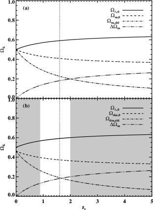
Figure 1: (a) Current relative magnitudes of vacuum density, $\Omega_{\Lambda,0}$, total density $\Omega_{m,0}$, the “old” matter density $\Omega_{m,old}$ and the “new” matter density $\Delta\Omega_{m}$ depend on $VDCR$, $z_{c}.$ (b) The same dependence for dark matter $\Omega_{dm,old}$ and $\Omega_{dm,0}$ with $\Omega_{B}$ fixed at the BBN value. Using priors on $\Omega_{dm,old}$ to put bounds on $z_{c}$ we constrain all the other quantities. The vertical dotted line gives results based on $\Omega_{dm,old}$ used to simulate recent (Wang 2001) best CMB fit.

At the other extreme it is possible that none of the decay products in $\Delta\Omega_{m}$ have yet deposited onto the bound matter in clusters. In that case the value of dark matter bound in clusters²⁴, $\left(\tilde{\Omega}_{m,0}-\tilde{\Omega}_{B}\right)\simeq 0.26(3)$, would be solely that due to the old dark matter $\Omega_{dm,old}\simeq 0.26(3)$. A look at Figure 1b shows that such a value corresponds to a lower bound on $VDCR$ of $z_{c}\simeq 0.89$. This, in turn, yields a lower bound on the decay products of $\Delta\Omega_{m}\simeq 0.13(3)$, an upper bound on total matter $\Omega_{m,0}\simeq 0.43$ (dark matter $\Omega_{dm,0}\simeq 0.39(6)$) and a lower bound on vacuum energy of $\Omega_{\Lambda,0}\simeq 0.57$. In Figure 1b, the shaded region on the left is disfavored by these constraints.

We can now summarize the constraints which, with the use of the selected priors, our model imposes on the cosmological parameters. Recall that central values of $\Omega_{dm,old}$ are used to choose the constraints and as such the latter are only intended to be illustrative. Given these assumptions, our model tells a story of a universe that started off with dark matter that now contributes a partial density $0.16\leq\Omega_{dm,old}\leq 0.26$. Recently, at a redshift of $0.89\leq z_{c}\leq 2.0$ the universe became vacuum dominated. Since then the decaying vacuum has produced matter. This new matter contribution presently amounts to $0.13\leq\Delta\Omega_{m}\leq 0.20$ with as much as $0\leq\left(\tilde{\Omega}_{dm,0}-\Omega_{dm,old}\right)\leq 0.10$ already deposited on to the clusters, leaving as much as $0.10\leq\left(\Omega_{dm,0}-\tilde{\Omega}_{dm,0}\right)\leq 0.13(3)$ to be inter-cluster unbound matter. The result is a vacuum dominated universe with a vacuum density $0.57\leq\Omega_{\Lambda,0}\leq 0.60$ and a total (including $\Omega_{B}$) matter density $0.40\leq\Omega_{m,0}\leq 0.43$.

C $D\Lambda-CDM$ and CMB

It is evident from this discussion of the $D\Lambda-CDM$ model that our knowledge of the present energy state of the universe would be considerably improved with tighter constraints on the primordial dark matter $\Omega_{dm,old}$. One unique tool to narrow down such constraints is the cosmic microwave background (CMB) radiation. The anisotropies in CMB are a powerful window into the early universe providing us with information about structure formation and cosmology in general²⁵. CMB has this ability because the amplitudes of its power spectrum (particularly the first peak) depend on the amount of dark matter that was available in the early universe to create gravitational potential wells into which the baryonic matter eventually collected. Moreover the heights of such peaks²⁶ in the power spectrum are not significantly affected by any (dark) matter $\Delta\Omega_{m}$ that might result from the effects of the recent domination of the universe by the vacuum ($>1000$ redshifts later). The only effect that such “new” matter will have on the CMB power spectrum is to shift, slightly, the horizontal (multipole) axis because of the expected $\Delta\Omega_{m}$’s lensing effects and the resulting change in the angular distance relationship. With the new combined data from BOOMERaNG, Maxima and DASI, the best fit simulations²⁷ seem to suggest a primordial dark matter content with a central value of $h^{2}\Omega_{dm,old}\simeq 0.1$.

Using this prior in our model (Figure 1b) we find a vacuum domination crossing redshift VDCR of $z_{c}\simeq 1.6$. Following the same arguments as before we see that the amount of matter produced from the decaying vacuum since $z_{c}$ would be $\Delta\Omega_{m}\simeq 0.18$. Out of this as much as $\left(\tilde{\Omega}_{dm,0}-\Omega_{dm,old}\right)\simeq 0.08$ would have already deposited on clusters, leaving as much as $\left(\Omega_{dm,0}-\tilde{\Omega}_{dm,0}\right)\simeq 0.1$ unbound in the inter-cluster voids. This gives a vacuum dominated universe with $\Omega_{\Lambda,0}\simeq 0.59$ and $\Omega_{m,0}\simeq 0.41$. Figure 1b (dotted vertical line) shows that these results, using as a prior $\Omega_{dm,old}$ associated with CMB best fit, fall well within the bounds described by the model. On the basis that CMB is our best probe of the early universe so far, we take these CMB-based results as our central values.

D Features and tests of the model

In closing this discussion it is worthwhile to ask what new features the $D\Lambda-CDM$ model introduces into cosmology and astrophysics. We start by noting that the model we have presented independently depicts a universe which is presently vacuum dominated. In Section 3 we discussed the asymptotic behavior of the equation of state for the dynamical and interacting vacuum fluid used in our model. Such behavior uniquely introduces some features in the dynamics of the universe. In our discussion we found that such an interacting vacuum should be defined by an equation of state that depends not only on the vacuum energy density but also generally on the interactions between the vacuum and matter fields. In the limit of vanishing matter fields (or weak field limit) we showed that the usual, locally Lorentz invariant, vacuum equation of state $p=-\rho$ is recovered. This result is usefull in as far as it suggests that the model meets this requirement of general relativity. Moreover, as the vacuum becomes dominant and accelerates the universe in the process, the matter production rate from the decaying vacuum also increases. Provided the matter creation window $\varepsilon$ is large enough, this in turn increases the amount of matter in the universe, effectively decreasing the vacuum to matter density ratio. In the process, the equation of state adjusts to produce less and less matter as the matter component of the universe starts to dominate. Such a newly matter dominated universe would then begin to decelerate. At the same time the matter production from the decaying vacuum becomes suppressed due to matter dominance in the equation of state, the matter fields are redshifting with the scale factor as $a\left(t\right)^{-3}$ which is again faster than the dynamical (false) vacuum that is redshiting as $a\left(t\right)^{-2}$. Thus soon or later the matter field density $\rho_{m}$ falls below the vacuum energy density $\rho_{\Lambda}$. At this point the universe re-enters a vacuum dominated phase, begins to accelerate again and to produce more matter in the process. This a state of affairs then depicts a universe that may be self-tuning, periodically entering and exiting inflationary phases. Such a self-tuning universe would be stable to vacuum-induced runaway accelerations.

Our model of a universe with interacting fluids also does suggest a conceptual explanation to the Coincidence Problem. The Coincidence Problem expresses our lack of a simple explanation to why the energy densities in the vacuum and matter are presently comparable¹, especially in view of the fact that recombination $\left(z\sim 1000\right)$ and structure formation could only have been possible if the early universe was excessively matter dominated. In $D\Lambda-CDM$ the matter fields redshift faster than the dynamical vacuum by $\frac{\rho_{m}}{\rho_{\Lambda}}\sim a\left(t\right)^{-1}$. If matter was in dominance at some point in the past-then, independent of the initial conditions, the two field densities eventually cross at $z_{c}$ as the vacuum takes dominance. We have seen in the previous section that the combined effects of matter production from the vacuum and the perturbations in redshifting of the fields, forces the latter to interact within a decaying envelope. As the universe expands, the amplitudes of the vacuum and the matter field densities then continue to approach each other as they also decrease. This approach may or may not have a local oscillatory character in time. If the fields have an oscillatory character then there will be repeated local periods in time when their amplitudes are comparable. In general, the above combined effects eventually make the fields comparable as the universe evolves towards some attractor stable state in the future. The answer to the “why now…?” part of the Coincidence Problem may then be “….because the universe is old enough.”

There are some features of the $D\Lambda-CDM$ which are potentially verifiable. The first has to do with the suggestion the model makes that the total matter density of the universe is more than that bound in clusters, with the excess, $\left(\Omega_{dm,0}-\tilde{\Omega}_{dm,0}\right)$, still unbound voids. Such smoothly distributed inter-cluster matter may be distinguished from the vacuum by use of candles like Type Ia supernovae¹. However, noting (from the priors used) that the predicted amount of smooth inter-cluster matter is only as much as $0.10\leq\left(\Omega_{dm,0}-\tilde{\Omega}_{dm,0}\right)\leq 0.13$ its presence could still be hidden within the error bars (see for example (Perlmutter 1999)) of current detection techniques. It is interesting to ask what our results look like if we hide the above smooth dark matter within the vacuum. Recall that in our model (and based on the priors used) we found a vacuum density $0.57\leq\Omega_{\Lambda,0}\leq 0.60$ and a total (including $\Omega_{B}$) matter density $0.40\leq\Omega_{m,0}\leq 0.43$. Clearly hiding $\left(\Omega_{dm,0}-\tilde{\Omega}_{dm,0}\right)$ elevates the vacuum density to $\Omega_{\Lambda,0}\simeq 0.7$ while equally suppressing the matter density to $\Omega_{m,0}\simeq 0.3$. Coincidentally, these values correspond to those of some currently popular cosmological models.

There is, however, a second feature of $D\Lambda-CDM$ related to inter-cluster matter that may be more readily testable. This has to do with the suggestion we make that the newly produced dark matter in $\Delta\Omega_{m}$ should readily respond to the long range gravitational potentials of clusters by moving directly towards the same clusters. As a consequence, observations of dark matter halos of clusters may fail to detect a simple clear cut-off in the radial component of the halo density profiles. Recent observations²⁸ of matter distribution in galaxies based on lensing  show that density profiles of the dark matter halos manifest no obvious cut-off, up to $300h^{-1}\,kpc$. While such preliminary results may not constitute a vindication of the $D\Lambda-CDM$ model they tend to favor rather than disfavor the model. A concrete verification of these predictions can only be achieved through extensive exploration of halos. It is hoped that future long range lensing projects²⁸ will shade some more light on this issue.

In the event that a fairly significant amount of  $\Delta\Omega_{m}$ may have accreted on to cluster dark matter halos then one more effect could be verified in the future, with more precise measurement techniques. In that case primordial (pre-recombination) dark matter $\Omega_{dm,old}$ will have a deficit with respect not only to the total present dark matter content $\Omega_{dm,0}$ but also to that observed²⁴ bound-in-clusters dark matter $\tilde{\Omega}_{dm,0}$. Such information would already be imprinted on CMB which is powerful probe into the early universe. One recalls that in adiabatic inflationary models¹⁷ primordial dark matter is essential for creating the gravitational potentials that the baryons eventually get drawn into, after recombination. This is the process of structure formation. The freely streaming photons, after last scattering, then carry all this information forever as amplitude perturbations in their power spectrum. In particular, the height of the first peak in the CMB power spectrum is very sensitive to the available amount of primordial dark matter $\Omega_{dm,old}$. On the other hand CMB does cleanly discriminate between pre- and post-recombination events. In particular, the height of the first peak would not be affected by any dark matter $\Delta\Omega_{m}$ created long after recombination and structure formation. The $\Delta\Omega_{m}$’s only possible effect on the CMB power spectrum would be to slightly shift the curve horizontally (along the multipole moments axis) because of the slight changes in the angular distance relation resulting from the lensing effects. Thus the effect to look for is that CMB data should consistently demand best fits that use slightly less dark matter $\Omega_{dm,old}$ than that traditionally observed $\tilde{\Omega}_{dm,0}$ in galaxies and clusters, by such standard techniques as X-ray surveys. It has been pointed out before by several experts (see for example²⁹) that CMB fits may be improved by initial (pre-recombination) low dark matter values. The recent CMB data, for example, seems to suggest best fits²⁹ with central values of $\Omega_{dm}h^{2}=0.1^{+.07}$. However even with central values as low as these the results still lie within the error bars of the usually quoted dark matter values. Thus, if the effect exists, it can only be isolated by future higher precision measurements.

V Conclusion

In the preceding discussion we have investigated the possible effects of a decaying vacuum energy density provided by a dynamical positive cosmological constant $\Lambda\left(t\right)$. On applying generalized energy conservation conditions one finds that such vacuum decay will produce matter fields. This matter production by a dynamical cosmological constant is triggered by the recent domination of the universe by vacuum energy. Our model also assumes inflation and big bang nucleothenthesis (BBN). With these assumptions we have written down several of the cosmological quantities, including the present fractional densities of matter $\Omega_{m,0}$ and vacuum $\Omega_{\Lambda,0}$ contents in the universe in terms of only one parameter, namely: the recent vacuum domination crossing redshift (VDCR), $z_{c}$. This dependence on $z_{c}$ makes these densities observable quantities. A central feature of this model is that the amount of matter $\Omega_{m,0}$ in the current universe is more than that $\Omega_{m,old}$ at the time of recombination by an amount $\Delta\Omega_{m}$ that has been created since vacuum domination at $z_{c}$. While this “new” matter is produced smoothly everywhere it could accrete onto clusters through the long-range gravitational potentials of the latter.

To relate our arguments to observation we first estimate when the vacuum comes to dominate the universe, by constraining $z_{c}$. This is done by establishing reasonable bounds on the primordial dark matter, $\Omega_{dm,old}$. In our calculations we apply only the central values of such bounds. Given these priors we constrain the vacuum domination crossing redshift to $0.89\leq z_{c}\leq 2.0$. Within these constraints we find that from $z=z_{c}$ to the present, the decay of dark energy should have created matter to the tune of  $0.13\leq\Delta\Omega_{m}\leq 0.20$ with as much as $0\leq\left(\tilde{\Omega}_{dm,0}-\Omega_{dm,old}\right)\leq 0.10$ already deposited onto the clusters, leaving as much as $0.10\leq\left(\Omega_{dm,0}-\tilde{\Omega}_{dm,0}\right)\leq 0.13$ to be inter-cluster unbound matter. Consequently, within these constraints, the $D\Lambda-CDM$ model finds that the universe is presently vacuum dominated with a vacuum density of  $0.57\leq\Omega_{\Lambda,0}\leq 0.60$ and a total matter density of $0.40\leq\Omega_{m,0}\leq 0.43$. Further, using as a prior the dark matter density that currently gives the best fit to the latest CMB data, we find that the results (Figure1, dotted vertical line) fall well within the boundaries we already established. When used as a prior the CMB based $h^{2}\Omega_{dm,old}\simeq 0.1$ predicts in our model a universe that has been vacuum dominated since $z_{c}\simeq 1.6$ and currently has a total matter density of $\Omega_{m,0}\simeq 0.41$ and a vacuum dark energy density of $\Omega_{\Lambda,0}\simeq 0.59$. We take these results as our central values.

In closing we summarize some of the new features the model introduces in cosmology. First, the model points to an existence of newly formed dark matter in the inter-cluster voids and suggests that some of this matter should already be accreting onto clusters through the latter’s long range gravitational potentials. There are two consequences of this. If some of the newly produced matter is indeed already leaking onto the cluster then the latter’s dark matter halos will be extended in space and demonstrate little or no clear cut-off in their radial density profiles. Secondly, if indeed a substantial amount of this matter has already landed then the amount of dark matter we observe bound in clusters will be greater than that needed to produce the best CMB fits by an amount that might have already deposited onto the clusters. The difference between these two values, if it exists, could still be hidden within the measurements’ error bars. A final feature of our model relates to the combined effect of the matter production by a decaying vacuum and the different rates namely, $a\left(t\right)^{-3}$ and $a\left(t\right)^{-2}$ at which matter and the vacuum respectively dilute with the scale factor. Such combination may create conditions for a universe in which the vacuum and matter densities evolve towards comparable and decreasing amplitudes. This suggests a conceptual explanation to the Coincidence Problem. It also implies that the universe may be stable to vacuum-induced runaway accelerations.

In order to establish the validity of such notions, it is evident that more work needs to be done including developing exact functional form of the equation of state. Such efforts are being undertaken and the results will be reported elsewhere.

Acknowledgement 1

This work was made possible by funds from the University of Michigan

References

- [1] S. Perlmumutter, et al, ApJ. 517 565(1999).
- [2] S. Weinberg, Rev. Mod. Phys. 61, 1 (1989); S. M. Carroll, astro-ph/0004075.
- [3] S. Coleman, Nucl. Phys. B, 307, 867(1988).
- [4] M. Özer and M. O. Taha, Phys. Lett. B171, 363(1986); M. Gasperini, Phys. Lett. B, 194, 374(1987); M. Özer and M. O Taha, Nucl. Phys. B, 287, 776(1987).
- [5] W. Chen and Y. S. Wu, Phys. Rev. D 41, 695(1990).
- [6] J. C. Calvalho, J. A. S. Lima, I. Waga, Phys. Rev. D, 46, 2404(1992).
- [7] I. Waga, ApJ, 414, 4361993).
- [8] M. Özer and M. O. Taha, Nucl. Phys. B, 287, 776(1987).
- [9] M. Özer, ApJ, 520, 45(1999).
- [10] P. Rastall, Phys. Rev. D, 6, 3357(1972).
- [11] T. Harko and M. K. Mak, Gen. Rel. Grav., 31, 849(1999).
- [12] J. A. S. Lima, Phys. Rev. D, 54, 2571(1996).
- [13] P. J. E. Peebles, S. Seager and W. Hu, astro-Ph/0004389.
- [14] I. Zlatev, L. Wang, P. Steinhardt, Phys. Rev. Letts., 82, 896(1999).
- [15] A. Jaffe, et al, astro-ph/0007333; N. A. Bachall et al, ApJ. 541, 1(2000).
- [16] D. Tyler, et al, astro-ph/0001318; S. Burles and D. Tyler, astro-ph/9803071; S. Burles, et al, astro-ph/9901157.
- [17] A. Balbi, Astro-ph/0011202
- [18] Wayne Hu, R. Barkana and A. Gruzinov, astro-ph/0003365.
- [19] M. Visser, Phys. Rev. D, 56, 7578(1997).
- [20] A. Guth, Phys. Rev. D 23, 347(1981).
- [21] A. R. Liddle, astro-ph/0009491; Also see Alan Guth, A. Linde, P. Steinhardt.
- [22] X. Wang, M. Tegmark, M. Zaldarriaga, astro-ph/0105091.
- [23] J. Overduin and W. Priester, astro-ph/0101484; P. Viana, astro-ph/0009492.
- [24] N. A. Bahcall et al Science 284, 1481(1999).
- [25] W. Hu and M. White, astro-ph9602019.
- [26] M. Zaldarriaga, private communication.
- [27] X. Wang, M. Tegmark, M. Zaldarriga, astro-ph/0105091.
- [28] P. Fischer, AJ 120, 1198F(2000).
- [29] M. Tegmark, M. Zaldarriaga, astro-ph/0004393; C. Miller, R. Nichol and D. Batuski, astro-ph/0105423.