Phase Mapping as a Powerful Diagnostic of Primordial Non-Gaussianity

Abstract

The identification and extraction of non-Gaussian signals is one of the main cosmological challenges facing future experimental measurements of the cosmic microwave background temperature pattern. We present a generalized statistical measure based on a novel technique representation of Fourier phases using the return map. We show that this method is both robust and powerful in comparison, for example, with morphological measures.

]

I Introduction

One of the key challenges facing modern cosmology is the complete statistical characterization of the primordial density fluctuations believed to be the seeds of the large-scale structure of the Universe we see today. According to the prevailing orthodoxy, these initial perturbations were generated as quantum phenomena during an inflationary epoch [1]. If this is the case they should display Gaussian statistics. Among other potentially testable consequences of this is that the small angular variations of the cosmic microwave background (CMB) sky should have the same statistical form [2, 3]. Testing the hypothesis of primordial Gaussianity using maps of the CMB thus provides an opportunity to make experimental tests of ideas about the physics of the early universe. It is also necessary to devise robust statistical descriptors for the identification of foreground contaminations and systematic instrumental artifacts.

Searches for non-Gaussian (NG) signals within the COBE-DMR data have yielded positive detections that are at least partly explained by systematics [4]. The need to devise more powerful statistical probes has been recognized and acted upon, with key ideas focusing on the bispectrum [5] and higher-order polyspectra [6, 7]. Some of these methods have been developed as far as practical implementation on real data sets [8]. These techniques are sensitive only to particular types of NG signal [9], so in this paper we present a new method that is both extremely general and extremely robust.

II Phase Mapping

One of the most basic properties of a Gaussian random field (GRF) [2, 3] is that the Fourier phases are random and uniformly distributed between 0 and $2\pi$. The Central Limit Theorem virtually guarantees that a superposition of a large number of Fourier modes with random phases will be Gaussian, so the random-phase hypothesis even serves as a definition of a form of Gaussianity.

Testing the randomness of measured phases therefore provides a direct diagnostic of the statistical form of a fluctuation field. There are, however, some problems in using phases as a statistic. The foremost is that they are circular variables, only defined modulo $2\pi$. Traditional measures of association, such as covariances of the form $\langle\phi_{\mbox{\boldmath$k$}}\phi_{\mbox{\boldmath$k$}^{\prime}}\rangle$, are based on the assumption that the related measure is linear and are therefore inappropriate. Another problem is that phases are direct indicators of the morphology and location of specific features [10], so are themselves not translational-invariant. As the first attempt to use phases as the basis of a statistical test, ref. [12] used a quantity formed by taking the phase differences of neighboring Fourier modes in $k$-space. This idea is the first step towards our new “phase-mapping” technique [13]. We counter the problem of the circular nature of the phases by applying phases on to a “return map”, as follows.

For a set of phases $\phi_{k}$ from the Fourier transform of a one-dimensional process, a possible return map is a plot of $\phi_{k}$ against $\phi_{k+1}$ (neighboring phases) for all available pairs $(\phi_{k},\phi_{k+1})$ up to the Nyquist frequency $k_{N/2}$ where $N$ is the length of the process [10]. When the phases are random this will be a scatter plot with points distributed randomly within the bounded square of both axes $[0,2\pi]$. For a realization of two or more dimensions, we can extend the return mapping between neighboring phases to any fixed scale $\Delta{\mbox{\boldmath$k$}}\equiv(\Delta k_{x},\Delta k_{y})\equiv(m,n)$ (so mapping of neighboring phases is simply the mapping for $|\Delta{\mbox{\boldmath$k$}}|=1$). Therefore, this method forces to test randomness between all pairs of $\phi_{\mbox{\boldmath$k$}}$ and $\phi_{{\mbox{\boldmath$k$}}+\Delta{\mbox{\boldmath$k$}}}$, for all fixed $\Delta{\mbox{\boldmath$k$}}$ scales in the Fourier domain. What results is a “super-map”, each pixel of which represents a return map with a fixed scale $\Delta{\mbox{\boldmath$k$}}$.

III Statistical Analysis of Phase Maps

Having rendered the phase information in a pattern onto the phase map, we have to consider the construction of a statistical test using it. Our null hypothesis at each $\Delta{\mbox{\boldmath$k$}}$ case is a random (Poisson) distribution on the mapping square, so the randomness of phases is tested through $2\times m_{\max}\times n_{\max}$ squares, where $m_{\max}$ and $n_{\max}$ are the maximal scale in $k_{x}$ and $k_{y}$ direction, respectively. For simplicity and computational ease [13], we apply a test (similar to the $\chi^{2}$ test) of the uniformity of the pixelized mapped phases for different scales $\Delta{\mbox{\boldmath$k$}}$ as follows. A mean $\chi^{2}$ statistic is defined as

$$\overline{\chi^{2}}=\frac{1}{M}\sum_{i,j}\frac{\big{[}p(i,j)-\overline{p}\big{]}^{2}}{\overline{p}}\equiv\sigma^{2}\overline{p},$$ (1)

where $M$ is the number of pixels on the return map, $\overline{p}$ is the mean value for each pixel, and $\sigma^{2}=(1/M)\sum_{i,j}\left[p(i,j)/\overline{p}-1\right]^{2}$ is the variance of the contrast of the return map.

The return mapping of random phases will result in a Poisson distribution over all the map squares. For a Poisson distribution of integer $p(i,j)$, its variance $\langle(\Delta p)^{2}\rangle_{\rm Poisson}=\sum_{p=0}^{\infty}(p-\overline{p})^{2}(\overline{p}^{p}e^{-\overline{p}}/p!)=\overline{p}$. Hence in this case $\overline{\chi^{2}}_{\rm Poisson}=1$, and from Eq. (1), $\sigma_{\rm Poisson}^{2}=(\overline{p})^{-1}$. One could use this result to test the return map for consistency with pure discreteness fluctuations. However, such a test is not so useful as it does not probe the spatial arrangement of the pattern. The individual return maps tend to display particular patterns to which this would not be sensitive. We could, for example, populate the pixels with a Poisson distribution of counts but then rearrange them arbitrarily over the grid without changing the statistical properties mentioned above. One could sort the counts in ascending order, for example, producing a clearly non-uniform distribution that has the same statistics as the starting case.

In order to apply this method more usefully we have to take into account the spatial correlations, which we can do using smoothing. For a 2D square $p(i,j)\equiv p({\mbox{\boldmath$x$}})$, we use the form

$$p({\mbox{\boldmath$x$}},R)=\int\frac{d^{2}{\mbox{\boldmath$x$}^{{}^{\prime}}}}{2\pi R^{2}}\>p({\mbox{\boldmath$x$}^{{}^{\prime}}})\>\exp\left(-\frac{|{\mbox{\boldmath$x$}}-{\mbox{\boldmath$x$}^{{}^{\prime}}}|^{2}}{2R^{2}}\right),$$ (2)

where $p({\mbox{\boldmath$x$}},R)$ is the smoothed square and $R$ is the smoothing scale.

To obtain the expectation value of $\overline{\chi^{2}}$ statistic of GRFs, we calculate first the variance of the contrast of the smoothed square, using a Gaussian window filter as in Eq. (2). For a 2D field with power spectrum $P(k)=Ak^{n}$, the variance of the contrast of the smoothed square [2] is $\sigma^{2}(R)=(A/4\pi)\Gamma(n+2/2)R^{-(n+2)}$, where $\Gamma(n)$ is the Euler Gamma function and $R$ is the smoothing scale in Eq. (2). A Poisson distribution has a power spectrum which is independent of wave number, i.e., its spectral index $n=0$. So originally the variance of the contrast $\sigma_{\rm Poisson}^{2}=A=(\overline{p})^{-1}$, after smoothing, becomes $\sigma^{2}_{\rm Poisson}(R)=(4\pi R^{2}\overline{p})^{-1}$. According to Eq. (1), we can obtain the $\langle\overline{\chi^{2}}\rangle$ from the variance of the smoothed return map and the $\overline{p}$, so for an ensemble of Poisson distributions, the expectation mean $\chi^{2}$

$$\langle\overline{\chi^{2}}\rangle=\frac{1}{4\pi R^{2}}.$$ (3)

Thus, any smoothed return map of phase pairs at a fixed $\Delta{\mbox{\boldmath$k$}}$ that generates a $\overline{\chi^{2}}$ value much higher than $(4\pi R^{2})^{-1}$ should be interpreted as a diagnostic of phase coupling at that particular scale in phase space. To apply phase mapping technique as a NG test, the null hypothesis requires that phase mapping for any fixed scale $\Delta{\mbox{\boldmath$k$}}\equiv(m,n)$ should result in Poisson distribution in a return map. Therefore, for a Gaussian realization, we have an ensemble of $2\times m_{\max}\times n_{\max}$ smoothed return squares which are subject to statistical fluctuations around $\langle\overline{\chi^{2}}\rangle$. Although phase mapping extracts all the information between phase pairs, we have to know whether the value obtained from $\overline{\chi^{2}}$ statistic is due to non-randomness or statistical fluctuation. As the $\overline{\chi^{2}}$ statistic is related to the ‘variance’ of the smoothed Poisson-distributed return map, the problem now is equivalent to finding the distribution of sampling variance from normal samples. The statistical significance of the departure of a measured value of $\overline{\chi^{2}}$ can be assessed using standard techniques for the sampling distribution of the variance in normal samples. When the sampling number is large enough, it behaves as Gaussian. We have $M$ independent variables $p_{i}-\overline{p}/\sqrt{\overline{p}}$, each of which is distributed normally with zero mean and variance $\langle\overline{\chi^{2}}\rangle$. We are now looking for the distribution of sampling variance $w\equiv\overline{\chi^{2}}=(1/M)\sum_{i}(p_{i}-\overline{p})^{2}/\overline{p}$, which can be obtained as [14],

$$dF=\frac{(M/2\langle\overline{\chi^{2}}\rangle)^{(M-1)/2}}{\Gamma[(M-1)/2]}\exp\left(-\frac{Mw}{2\langle\overline{\chi^{2}}\rangle}\right)w^{(M-3)/2}dw.$$ (4)

Therefore, the variance of the sampling $\overline{\chi^{2}}$ measurements ($M\gg 1$) is $\Sigma^{2}=\int_{0}^{\infty}(w-\langle\overline{\chi^{2}}\rangle)^{2}dF=\langle\overline{\chi^{2}}\rangle^{2}/(M/2)$. The dependence of $\Sigma^{2}$ on $R$ can be obtained through Eq. (3), and the change of the effective pixel number $M$ to $(\pi/2)^{2}M/(4\pi R^{2})$ due to smoothing. Therefore,

$$\Sigma^{2}=\frac{1}{\pi^{3}R^{2}(M/2)}.$$ (5)

We can examine NG signals in two ways. A pixel in the “super-map” which corresponds to $\nu\Sigma$ with $\nu\simeq 5$, say, would be extremely unlikely if the null hypothesis held. As well as easily identifying such hotter pixels, we can also retrieve the corresponding $\Delta{\mbox{\boldmath$k$}}$ scale of the signal from the map. One could look at modes flagged in this way more carefully using other statistics if necessary. On the other hand, we can also inspect the global property of the distribution curve with $\langle\overline{\chi^{2}}\rangle$ and $\Sigma$ when the number of $2\times m_{\max}\times n_{\max}$ is large. Even when all signals are below $5\Sigma$, the underlying obscure NG part could cause the distribution curve to skew, albeit no signal is above $5\Sigma$ due to possible ’Gaussianization’ by the noise.

IV Application to simulated CMB maps

We apply this method to a simulated NG CMB map (Fig.1(a)), which is a realization of $12.8\deg^{2}$ CMB anisotropies due to the Kaiser-Stebbins effect from cosmic strings [11]. We will test the non-Gaussianity by applying our method not only directly to the original manifestly NG map (S), but also to the combined map of itself plus Gaussian white noise (N) with 5 different fluctuation levels, as NG part may be embedded in white noise. The Gaussian white noise level are chosen with rms ratio ${\rm S/N}=8$, 4, 2, 1 and 1/2.

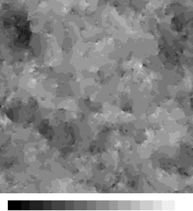
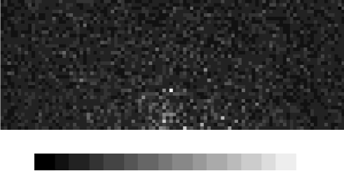
FIG. 1.: The temperature map ($\mu k$) and the “super-map”, in which each point represents the $\overline{\chi^{2}}$ value for that $(m,n)$ scale. The histogram of the latter is shown in Fig. 2 (a).

From the Fourier transform of a $N^{2}$-mesh realization, we have $N^{2}/2$ valid modes: $k_{x}\in[-N/2+1,N/2]$ and $k_{y}\in[1,N/2]$. In general, the phase basis used to extract NG signals is flexible with the constraint $|{\mbox{\boldmath$k$}}|_{\max}+|\Delta{\mbox{\boldmath$k$}}|_{\max}\leq k_{\rm Nyquist}$. We have taken phases from the inner quarter of valid modes as a basis, i.e., $k_{x}\in[-N/4+1,N/4]$, and $k_{y}\in[1,N/4]$. As the Gaussian noise normally dominates the power spectrum at large $k$’s, we can opt to avoid that part of ‘Gaussianized’ phases by shrinking the upper limit $|{\mbox{\boldmath$k$}}|_{\max}$ of the phase base (not the upper limit of $(m,n)$).

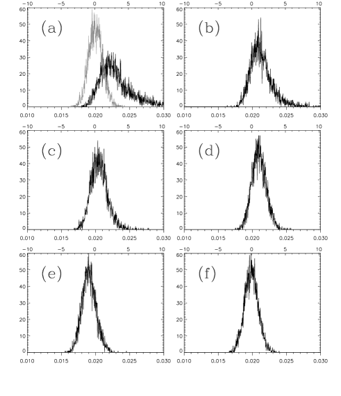
FIG. 2.: The histogram of $\overline{\chi^{2}}$ statistics. Panel (a) is from the pure temperature map caused by cosmic strings of Kaiser-Stebbins effect. For comparison, the gray curve is from a realization of (random-phase) GRF. Panel (b), (c), (d), (e) and (f) are the histograms for the combined map of CMB plus Gaussian white noise with rms ratio ${\rm S/N}=8$, 4, 2, 1 and $1/2$, respectively. The upper horizontal axis is annotated in terms of the theoretical value $\Sigma$ of GRFs with origin set at $\langle\overline{\chi^{2}}\rangle=(4\pi R^{2})^{-1}$. The smoothing scale on the $M=128^{2}$ pixelized return map is $R=2$. Therefore we regard those above $5\Sigma$ as against the null hypothesis, thus manifestation of phase coupling. We can see that phase mapping is able to detect considerable signals above $5\Sigma$ for the added Gaussian noise ${\rm S/N}=4$ and some for ${\rm S/N}=2$. Note that albeit no signals above $5\Sigma$ in (e), the median is shifted away from the $\langle\overline{\chi^{2}}\rangle$ value, which is also NG manifestation.

In Fig. 2 we show the histogram of the measured $\overline{\chi^{2}}$ statistics. Those above $5\Sigma$ are caused by phase coupling of some $\Delta{\mbox{\boldmath$k$}}$, which can be viewed in the $(m,n)$-map as in Fig.1 (b). As a NG test, we are interested only in the amplitude of phase coupling in terms of $\overline{\chi^{2}}$, whatever the $\Delta{\mbox{\boldmath$k$}}$.

V Comparison to the Analysis of Minkowski Functionals

We now compare this method with a more standard morphological analysis of temperature contours, based on Minkowski functionals (MFs). The 3 MFs in 2D are the area ($V_{0}$), circumference ($V_{1}$), and the Euler characteristic ($V_{2}$) of excursion regions [15]. The excursion region is the region on the sky map above a certain threshold amplitude [16]. In Fig. 3 we show the 3 MFs for the noise-contaminated cases: CMB plus noise with ${\rm S/N}=4$ and 2 shown by solid curves. The shaded areas are from $10^{3}$ realizations of the same power spectrum of the corresponding noise–contaminated CMB map but with random phases, which thus represents the statistical fluctuations of GRFs. We avoid quoting $1\sigma$ around the mean MFs as the distribution function for each threshold is not normal (e.g. for high thresholds $\nu$, $V_{2}\propto\nu\;e^{-\nu^{2}/2}$ [3]). The case of ${\rm S/N=4}$ is out of the shaded area, a definite NG manifestation, but ${\rm S/N=2}$ is right on the edge. The dashed curves are taken from one Gaussian realization in order to show the variation of the MFs and the ambiguity that would result.

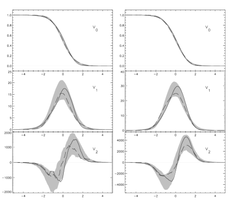
FIG. 3.: Minkowski functionals for the combined temperature map with ${\rm S/N}=4$ (left column) and ${\rm S/N}=2$ (right) in solid curves against threshold (in terms of rms). From top downwards are the area, circumference and the Euler characteristic. The shaded areas are the possible ranges for each functional from $10^{3}$ realizations of the same power spectrum (as the noise–added CMB map) but random phases and the dash curves are from one of the $10^{3}$ Gaussian realizations.

Other types of NG signals localized in harmonic space, e.g., artifacts from systematics such as slowly–rotating elliptical beam of the planck mission will produce NG signals around $\ell_{\rm pix}$, which is more easily detected with harmonic analyses than real-space ones. By “localized in harmonic space” we mean the phases correlate mainly from large $k$. The contrary example is the simulations of spectral index $n=2$ [13], where phases correlate first at large $\Delta{\mbox{\boldmath$k$}}$ from all $k$.

These results show that the phase-mapping technique is able to detect certain forms of non-Gaussianity even in the presence of noise, more effectively than the MF approach. The theoretical ground for phase mapping we have developed as a powerful NG diagnostic can be directly applied not only on spherical analysis, but also on time-ordered scans of the upcoming planck mission.

This paper was supported in part by Danmarks Grundforskningsfond through its support for the establishment of TAC by grants RFBR 17625. PC acknowledges support from PPARC. We are grateful to A. A. Starobinsky for useful discussions.

REFERENCES

- [1] A. A. Starobinsky, Phys. Lett. , B91, 99 (1980). A. H. Guth, Phys. Rev. D., 23, 347 (1981). A. H. Guth and S.-Y. Pi, Phys. Rev. Lett., 49, 1110 (1982). A. Linde, Phys. Lett. , B108, 389 (1982). A. Albrecht and P.J. Steinhardt, Phys. Rev. Lett., 48, 1220 (1982). A. A. Starobinsky, Pis’ma Zh. Eksp. Teor. Fiz., 30, 719 (1979). V. Mukhanov and G. Chibisov, ibid. 33, 532 (1981). A. A. Starobinsky, Phys. Lett. , B117, 175 (1982).
- [2] J. M. Bardeen, J. R. Bond, N. Kaiser, and A. S. Szalay, Astrophys. J., 304, 15 (1986).
- [3] J. R. Bond and G. Efstathiou, Mon. Not. R. Astron. Soc., 226, 655 (1987).
- [4] P. G. Ferreira, J. Magueijo and K. M. Gorski, Astrophys. J., 503, L1 (1998). J. Pando, D. Valls-Gabaud, and L. Fang, Phys. Rev. Lett., 81, 4568 (1998). B. C. Bromley and M. Tegmark, Astrophys. J., 524, L79 (1999). J. Magueijo, Astrophys. J., 528, L57 (2000).
- [5] X. Luo, Astrophys. J., 427, L71 (1994). A.F.Heavens, Mon. Not. R. Astron. Soc., 299, 805 (1998). L. Verde, L. Wang, A.F. Heavens, and M. Karmionkowski, ibid. 313, 141 (2000); L. Verde, R. Jimenez, M. Kamionkowski, and S. Matarrese, ibid. 325, 412 (2001).
- [6] L. Verde and A. F. Heavens, Astrophys. J., 553, 14 (2001). W. Hu, Phys. Rev. D., 64, 083005 (2001).
- [7] A. J. Stirling and J. A. Peacock, Mon. Not. R. Astron. Soc., 283, L99 (1996). A. Cooray, Phys. Rev. D., 64, 043516 (2001). H. Eriksen, A. Banday and K. Gorski, astro-ph/0206327.
- [8] N. G. Phillips and A. Kogut, Astrophys. J., 548, 540 (2001). H. B. Sandvik and J. Magueijo, Mon. Not. R. Astron. Soc., 325, 463 (2001). E. Komatsu et al., Astrophys. J., 566, 19 (2002). M. G. Santos, et al., Phys. Rev. Lett., 88, 241302 (2001).
- [9] P. I. R. Watts and P. Coles, Mon. Not. R. Astron. Soc. submitted.
- [10] L.-Y. Chiang and P. Coles, Mon. Not. R. Astron. Soc., 311, 809 (2000). L.-Y. Chiang, ibid. 325, 405 (2001). P. D. Naselsky, D. I. Novikov, J. Silk, Astrophys. J., 655, 565 (2002).
- [11] F. R. Bouchet, D. P. Bennett, and A. Stebbins, Nature (London), 335, 410 (1988).
- [12] P. Coles and L.-Y. Chiang, Nature (London), 406, 376 (2000).
- [13] L.-Y. Chiang, P. Coles, and P. D. Naselsky, Mon. Not. R. Astron. Soc. accepted, astro-ph/0207584.
- [14] M. G. Kendall and A. Stuart, The Advanced Theory of Statistics (Charles Griffin & Company Limited, London, 3rd ed. 1973), Vol. 1, p.273.
- [15] K. R. Mecke, T. Buchert, and H. Wagner, Astron. Astrophys., 288, 697 (1994). J. Schmalzing and K. M. Gorski, Mon. Not. R. Astron. Soc., 297, 355 (1998).
- [16] P. Coles and J. D. Barrow, Mon. Not. R. Astron. Soc., 228, 407 (1987). P. Coles, ibid. 234, 509 (1988).