New algorithms and technologies for the un-supervised reduction of Optical/IR images

Abstract

This paper presents some of the main aspects of the software library that has been developed for the reduction of optical and infrared images, an integral part of the end-to-end survey system being built to support public imaging surveys at ESO. Some of the highlights of the new library are: unbiased estimates of the background, critical for deep IR observations; efficient and accurate astrometric solutions, using multi-resolution techniques; automatic identification and masking of satellite tracks; weighted co-addition of images; creation of optical/IR mosaics, and appropriate management of multi-chip instruments. These various elements have been integrated into a system using XML technology for setting input parameters, driving the various processes, producing comprehensive history logs and storing the results, binding them to the supporting database and to the web. The system has been extensively tested using deep images as well as images of crowded fields (e.g., globular clusters, LMC), processing at a rate of 0.5 Mega-pixels per second using a DS20E ALPHA computer with two processors. The goal of this presentation is to review some of the main features of this package.

European Southern Observatory, Karl-Schwarzchild-Str. 2, D-85748 Garching bei Munchen, Germany.

1 Introduction

The ESO Imaging Survey (EIS) [3] project at ESO is an ongoing effort to conduct public imaging surveys and to develop the required infrastructure and software tools to support the large volume of optical/infrared data expected from such surveys, using dedicated imaging telescopes such as VST and VISTA.

Since 1997 EIS [10] has conducted a variety of medium-size optical/infrared surveys. The challenge has been to cope with the variety of imagers and observing strategies and, more recently, with the large volume of data coming from the wide-field imager (WFI) mounted on the 2.2 m telescope at La Silla. In the early phases of this project the main effort was to adapt existing software to the project’s particular needs leading to the use of different packages (e.g., IRAF, ECLIPSE). This made it difficult to develop a common environment for operations. Therefore, for the past two years an effort has been made to develop a common, end-to-end, integrated system capable of supporting un-supervised reduction. From the EIS survey system it is possible to prepare observations, retrieve raw data and convert these to science grade products in the form of fully calibrated pixel maps, catalogs and other derived products [6]. This effort has progressed in several fronts and includes the development of an administrative wrapper using Python, graphic user interfaces (Tcl/Tk), the integration of a supporting database (Sybase), a suite of survey tools and an image processing package.

Coping with the large volume of data expected in the future, and the multi-wavelength nature of the public imaging surveys currently being conducted requires the image reduction software to have a high-throughput and to be instrument-independent. This has been accomplished using a new, C-based library which integrates XML technology and a host of new algorithms to deal with a variety of situations encountered in observations covering the optical and infrared domains, while using single- and multi-chip instruments. Here a brief review of the main concepts and algorithms is presented.

2 Preparation Steps for Reduction

As stated earlier, the software developed is capable of supporting single-CCD or multi-CCD instruments, and a variety of electronic layouts (several over-scan areas and read-out ports). To support an instrument the system requires the following information. First, a list of basic keywords (seven in total) in the FITS header of the original must be translated into those recognized by the system. All others are re-computed as required to conform to the internal convention and ensure consistency throughout the processing phase. Second, information about the camera used such as: the number of CCDs, their geometric layout in the array, and the electronic layout of each CCD. The electronic layout is defined by the location of the overscan areas, and the number, location and properties (read-out noise and gain) of different read-out ports. These define different quadrants on the image, which must be known for a proper reduction. Third, the definition of Reduction Modes (RM; see section 4) specific to that instrument.

Once this information is available and the raw data are on disk the process can start. The first step is to check the number of fits extensions in the raw images. If this number corresponds to the number of CCD chips expected for the instrument, the original raw image is split into individual ones. The second step is to translate the keywords in the fits header of the raw images, using the dictionary mentioned above, and to check for their existence and integrity. The third step is to organize the raw images by recognizing their types (science, standards, calibration) and to create reduction blocks (RBs). These consist of groups of images taken sequentially and sharing the same filter and/or position (in the case of science images). Calibration frames are also sorted by their type namely bias, dark, dome flats and twilight flats. Dark exposures with the same integration time are grouped together. These calibration RBs can be further combined according to a period of validity defined by the user. Finally, each RB is assigned a RM which tells the system how these images should be reduced and the parameters to use for each sub-process.

The reduction mode carries information about the instrument (number of chips, chip size, overscan region, read-out ports, gain, readout-noise) and attributes such as the type of image (dark, bias, flat, standard, science), type of survey (extragalactic or galactic fields), and passband (optical/infrared). Each of these attributes may require a special sequence of processes and/or suitable parameters. The information contained in the RB is used to define the sequence of processes and the optimal parameters for each instrument and passband. The present system is capable of sorting out these various pieces of information and use the specific modules required with the appropriate set of parameters. To a large extent this is the major advantage of an integrated system as the one described here.

For science frames, besides the RB, one has also to provide additional information such as the astrometric reference catalog to be used in the registration of the images and the definition of a reference grid onto which the final reduced images will be mapped. This reference grid is defined by a reference sky position, a pixel scale and orientation (e.g., north-up; east-left) and a projection (e.g., TAN, COE). The use of a reference grid is not mandatory but is recommended for deep observations and mosaics since it is easier to co-add images sharing the same grid convention.

In the survey system version, the Python wrapper can use the original groups and apply additional constraints to filter out images. For instance, it is possible to restrict images based on the variation of the seeing (currently based on the values of the seeing monitor), the time or airmass interval covered, and enforce that the reduction block corresponds to the original observation blocks (OB), as defined by ESO’s data flow system.

Before the actual reduction of the data, some additional checks are required. The first check is on the accuracy of the reference pixel stored in the header. This is important in order to detect possible large offsets from the expected location which may occur due to changes in the pointing model at the telescope. This is also critical given the convention adopted by ESO for the CRVALs and CRPIXs values in the FITS header of the raw images (especially SUSI2and WFI). This check is carried out using a cross-correlation technique between two images. The first is a low-resolution (under-sampling by a factor of 8 the original pixel scale of the CCD considered) version of a mock image created from the reference catalog drawn from a much larger area than one CCD (ranging from 4 to 36 times the original field-of-view). The other is constructed from the science image to the same resolution as the one adopted earlier using wavelet transform, padded with zeros to match the mock image size. In preparing the low-resolution science image, care must be taken to remove cosmic rays and the effect that a few bright stars may have on the results. A more detailed description of the method will be presented in a forthcoming paper. The peak of the cross-correlation yields the offset that must be applied to the values of CRPIXs in the header to correspond to the values of the CRVALs. This correction is then applied to all frames (individual chips) belonging to the same night or an arbitrary period of validity specified by the user. This procedure is possible thanks to the speed of the algorithm which works with low-resolution images and benefits from the Fast Fourier Transform (FFT). One advantage of carrying out this reference pixel check at the preparation phase is to assure that during reduction only a refinement of the astrometric solution is required. Note, however, that the method is only valid for correcting translations. When dealing with multi-chip instruments some algorithms (see section 3) require information about the exact location of each chip and this must be checked by the system. Since it is not advisable to rely in the order in which they appear in the FITS file, which may (have) change in time, this must be computed. Once new CRPIX values are available these are used to define the geometry of the array and to cross-check if the computed CRPIXs are consistent.

3 Handling Calibration Frames

Normally, the first RBs to be reduced are those associated with the calibration frames. However, it is also possible to assign external master calibrations, in which case this step can be skipped. Each calibration RB of the “closed” type (dark and bias) containing at least three frames a median value is computed and a master bias and dark are created following the validity period specified. Several master darks may exist with different exposure times. In general, darks are only used for IR reduction, since their contribution for modern optical CCDs is negligible. The RB for flats (dome or twilight) contains only frames within a specified range of counts, the others being rejected in the preparation phase. Each frame is then subtracted by the master bias or, in the case of IR, by the corresponding (same exposure time) master darks. Each frame is then divided by their mean to provide normalized images and a median value is computed to produce the master flat. The same procedure is adopted for dome and twilight flats, but currently for test reductions the twilight flat is normally used leading to good results. One exception is the IR images taken with SOFI at La Silla. SOFI uses the so called special-flats, requiring a special reduction procedure which is currently not yet available. Instead the flats prepared on the mountain are used.

Once a master flat is available a bad-pixel (hot/cold/dead pixels) map is created by flagging pixels with intensities greater or smaller than a threshold level on an image storing the difference between the master flat and a smooth version of it produced by computing a median in a 10$\times$10 box. This is done automatically and on-the-fly for each reduction with no need for saving this map. At this point the information about the read-out ports is important in order to avoid smoothing over the border of different quadrants. Otherwise these borders will be flagged as bad-pixels.

The master flat also characterizes the noise level of the pixels which can be used to define the notion of weight map (pixels with a low efficiency should have a smaller signal-to-noise). This notion is critical in the co-addition of images and for a homogeneous source extraction at a fixed signal-to-noise level. The weight map is equal to the master flat. It can also be generalized by multiplying it by the bad-pixel map which gives zero weight to the rejected pixels. This weight map is then associated to all raw science frames within the validity period of the master flat. It is important to emphasize that the weight map is equivalent to an effective exposure map.

The procedure described above also applies to multi-CCD instruments, with the system splitting the raw images into individual CCDs. The administration of these several files is carried out internally by the system and it is transparent to the user. However, for CCD arrays an additional step is necessary, namely the correction for variations of the gain from chip-to-chip along the array so as to enforce that all the master flats of the different CCDs have the same gain.

This correction is computed separately and for each filter using long exposures and assuming that all CCDs in the array have the same gain. Hence, after they are corrected for instrumental effects (bias, dark, flat), they should share the same background value. Under this assumption the background is computed at the four borders (left, top, right, bottom) of each CCD in the array. If differences in the counts are found, a flux-scaling factor for each CCD is computed such as to minimize these differences. The flats are then multiplied by the derived flux scale. For the instruments considered (e.g., SUSI2, WFI) these differences are typically less than 10%. It is important to note that this calculation does not take into account nor corrects for illumination effects. The derivation of the illumination correction needs to be done separately and it is not yet fully implemented.

In principle, this procedure prevents the need for the calculation of independent photometric calibrations for each chip. However, the robustness of the procedure must be independently monitored by computing photometric solutions chip by chip. Such a facility is provided by the survey system.

4 Handling Science Frames

4.1 Reduction

The pipeline offers different ways to process a reduction block of raw images. As mentioned earlier these are set by the Reduction Mode (RM) assigned to it. In the present framework four main modules are available as schematically shown in Figure 1. Also indicated at the bottom are the external dependencies (e.g., master calibration images and chip layout, weight map, and reference catalogs for the absolute astrometric solution) of each of the modules. The current system consists of the following steps:

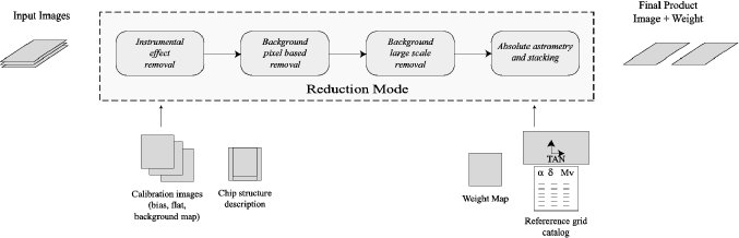
Figure 1: Main available steps of a Reduction Mode.

• Removal of instrument signature - For each optical image the master bias is overscan corrected quadrant by quadrant and subtracted from the science images. Next the science images are divided by the master flat. A similar procedure is adopted for the IR images except that instead of the master bias, the master dark with the appropriate exposure time is used. An option is available to interpolate across bad pixels. In general, however, since multiple exposures are available this is taken into account by the weight map during the co-addition process.

• Removal of local background - this module is normally used to deal with images observed in passbands where both low and high-frequency features such as fringes are present in the background. This is typically the case for the red passbands in the optical (R and more conspicuously in I) and in the infrared domains. A first crude attempt to estimate the local background is done by assuming that the observed features are stable in pixel coordinates. A first estimate of the local background level is computed as the median of the the intensity of all images in the RB at that pixel. Next all images in the RB are subtracted by this estimated background. However, as shown in sub-section 5.1 this estimate is bias and greatly affects the flux of faint objects. To improve the background estimate it is necessary to mask out objects. In order to do that the images are registered using one of them as reference, and the values are added and divided by the number of images contributing at the position of the pixel in the new grid. Objects are extracted from this image and a mask image is created. This mask is then applied to the original images in the RB at their original pixel coordinates. Pixels inside the masks are then discarded in the calculation of the mean for a second estimate of the background. This second estimate is then used to subtract the background of each image. The resulting RB is then used by the next module. In cases where there are not enough exposures or for very crowded fields the system uses an external fringing map as discussed in sub-section 5.1.

• Removal of low-frequency background - this module computes and removes the background of each image. This procedure assumes that the images have a smooth background (using a median of a top-hat filter) and that the smoothing scale is larger than the largest object in the image. For each image a mini-background is computed (according to the smoothing scale adopted) and an estimate of the background, for each quadrant, is computed merging a user specified number of mini-backgrounds. Once this estimate is available the mini-backgrounds are re-sampled back to the original image scale and subtracted from all images in the RB. In the case of IR observations carried out in nights of variable conditions, it is recommended to deal with each image separately. At this point any residual imprint of the quadrant structure in the CCD is removed.

• RB stacking & Astrometric calibration - the final module of the reduction part is responsible for producing a final image which combines all the images in the RB, normalized to one second integration time (and computing an effective gain), by calculating the mean value at each location, and astrometrically calibrating the final image. The noise of the normalized images in the RB are computed and for RBs with at least three images the noise distribution is examined and outliers are removed. In case the individual images have sufficient high S/N objects, the astrometric reference catalog specified in the previous section is used to create a mock image (as discussed above) using the reference grid specified at the preparation level, to determine the absolute astrometric registration for each image which are warped and then combined. This is normally the case used for optical images with exception perhaps of usually shallower $U$-band exposures. For the latter and for all IR images a relative astrometric solution is found, images are then warped and combined. This final image is then astrometrically calibrated using the reference catalog mapped (warped) to the final reference grid, exactly in the same way as above. Once the images in the RB are registered (absolutely or relatively) cosmic rays are removed using a sigma-clipping technique. At this point, the Hough transform (see sub-section 5.3) is applied to identify possible satellite tracks. If found, pixels along a strip surrounding the track are rejected. Finally, the weight map is used to mask out bad pixels. This is done before warping the images. In general, this module deals with sky-subtracted images coming out from the previous modules. However, this is not required since in some cases it is of interest to keep the smooth part of the original image background. On the other hand, this module can only be used after fringes have been removed, since they greatly impact the wavelet decomposition, specially in the medium-resolution scales which is used for the first estimate of the astrometric calibration. In the case of images for which the background has not been removed, offsets in the background level, due to variations in sky brightness during the time interval of the RB, are corrected for using one of the images as reference. The final stacked image is trimmed according to a user specified minimum number of contributing images. The weight map of the final image is the sum of the original weights properly normalized and warped, taking into account the exposure times of the original images.

Typical examples of reduction modes are: 1) deep IR images and optical images in I-band all modules are active; 2) in the case of the bluer passbands, the local background module can be bypassed; 3) in the case of crowded fields, such as those in the Pre-Flames survey, only the first and the last modules are used.

4.2 Final Products

Often the observations are carried out as a sequence of OBs. Therefore, at the end of the reductions several reduced RBs are available all sharing the same reference grid. At this point these intermediate images can be combined using the weight maps and the noise, as weight. At this stage a further rejection of cosmic rays is applied leading to the removal of lower S/N features not detected in the original frames. In the case of multi-chip instruments at the end of the process the RBs of the individuals CCDs are merged together into the final image as specified by the reference grid. This assumes that flux scaling correction of the flats described earlier is adequate. Otherwise, an external correction factor for each CCD has to be provided and an external module has to be used to combine and merge the different chips.

5 Algorithms

5.1 Removal of Fringes

As mentioned in the previous section fringes are a common phenomenom present on near-infrared images. Fringes are an additive signal stemming from sky emission lines, making a non-negligible contribution to the total signal, typically of the order of 10% of the background level. Hence, subtracting its contribution is essential for a proper reduction of the image. While in the optical, the fringing pattern is relatively stable (but exceptions exist) over the time scale of a night, in the infrared the fringes vary very quickly. Fortunately, the fringing pattern is largely independent of the pointing and consecutive images share the same pattern. This allows them to be separated from the astronomical objects by shifting the pointing observations. While the objects will fall in different pixel locations the fringes will not.

Therefore, a first crude estimate of the fringing pattern is to compute the median at every pixel using the estimator $E$ given by

$$B_{i,\,j}\,=\,E\,\left(P_{n_{i,\,j}-}\mu_{n},\,\forall n\right)$$ (1)

where $B_{i,\,j}$ is the computed background at the location $(i,\,j)$, $P_{n_{i,\,j}}$ is the counts of the pixel $(i,j)$ of the $n^{th}$ image, and, $\mu_{n}$ is the mean of the $n^{th}$ image. Subtraction of $\mu_{n}$ is important because it may vary from one image to another in the case of non-photometric nights. The estimator apply on the RB is shown in Figure 2 on the left panel.

Unfortunately, this estimator is biased due to the presence of faint astronomical objects which cannot be detected in the individual images due to their low S/N. However, if all images are combined these objects can have a significant contribution. For instance, for an RB with 60 images objects detected in the final image with a S/N $\sim$ 2 have a S/N $\sim$ 0.25 on the individual images. Neglecting their contribution in estimating the background leads to an overestimate of the background, and consequently to an underestimate of the flux of the objects. This effect can be as large as 0.2 mag near the limiting magnitude.

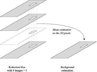
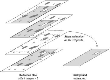
Figure 2: An illustration of the two methods used to estimate the background: Left: a simple median filtering; Right: median filtering after masking objects in the final stacked image, as described in the text.

In order to improve the estimator $E$ in equation (1) it is necessary to distinguish pixels which have the “background value” from those contaminated by the light of objects as illustrated in the right side of Figure 2. In order to do that one has to use the first estimate of the background, combine the sky-subtracted images, detect objects, and create masks which encompass surrounding pixels containing the object. These masks are then mapped back to the individual images and used to discard pixels in a second estimate of the background. Typically, the mask size is taken to be about twice the estimated size of the objects. The estimator apply on the RB with the mask is shown in Figure 2 on the right pannel.

If the background is evolving during the total exposure time, it can be estimated only from some images observed consecutively. The algorithm allows to specify a range of images to be used to estimated the background. In the IR the background is evolving faster, and a range of typically 15 images is used to compute the background, corresponding to 15 minutes of observation.

One limitation of the method is that, for large objects and very dense regions it may be impossible to “see” the sky, in which case holes will appear in the final image. In order to avoid this case a proper choice of the amplitude of the jitter pattern is critical.

5.2 Astrometric registration using wavelet transform

In the pipeline astrometric solutions are computed either in a relative or in an absolute way. For instance, relative astrometry is done for the stacking of an RB using one of the images as reference, while an absolute astrometric calibration requires an astrometric reference catalogue and a grid. In both cases the solution is found using the concept of multi-resolution (reference), by comparing low-resolution images obtained from a wavelet decomposition. In the case of a reference catalog this is done by first creating a mock image to map the objects listed in the catalog onto a reference image according to the grid convention. This method is referred to as pixel-based image registration [4].

The calculation of the geometrical distortion between the two images requires: 1) the identification of a set of well defined astronomical objects (control points, hereafter CP) in both images; 2) the definition of a functional form for the deformation model which maps a point $(x,y)$ in the input image to a point $(X,Y)$ on the reference image; 3) the creation of the distorted or corrected image, which requires the adoption of an interpolation or warping method.

The distortion model adopted by the pipeline is a pair of bivariate polynomials given by:

$$\left\{\begin{array}[]{ccc}X_{i}&={\displaystyle\sum_{p=0}^{N}\sum_{q=0}^{N-p}}\,a_{pq}\,x_{i}^{p}y_{j}^{q}=&P\,(x_{i},y_{i})\\ Y_{i}&={\displaystyle\sum_{p=0}^{N}\sum_{q=0}^{N-p}\,b_{pq}\,x_{i}^{p}y_{i}^{q}}=&Q\,(x_{i},y_{i})\end{array}\right.$$ (2)

Where $\textrm{(}X_{\textrm{i}},Y_{i})$ are the coordinates of the $i^{th}$ CP in the reference image and $(x_{i},y_{i})$ the corresponding CP from the input image. $N$ is the degree of the polynomial. Usually, the degree of the polynomial is one or two for instruments with a small field-of-view and up to four otherwise. Then follows the computation of the unknown parameters ($\frac{(N+1)(N+2)}{2}$ for each polynomial) using the least mean square estimator (LMSE).

The most difficult step of the process is to associate the CP from the input image with the CP from the reference image. CP are randomly spread and can be very dense. The associations cannot be done using any window search because multiple associations will occure and will bias the distortion estimation. The idea of the wavelet transform, is to work with different resolutions and therefore give a constraint for the minimum distance between CP.

Let $I_{r}$ be the reference image and $I_{i}$ be the input image. On each image the wavelet transform with the so called algorithm à trous [8] is performed up to the scale $L$ producing two wavelet images $W_{il}$ and $W_{rl}$ with: $l\,\in\,(1,L)$ from the two images $I_{i}$ and $I_{r}$. $L$ being the initial dyadic step, it corresponds to the large details of the images. A detection procedure on $W_{iL}$ is achieved and only the local maxima with amplitude greater than three times the sigma of the noise are kept. Theses local maxima play the role of CP. They correspond to significant image patterns, and have to be found in the corresponding wavelet plan of the reference image $W_{rL}$. The association is done with a window search. The search radius is set to $2^{L-1}$ pixels, and corresponds to the half of the maximum wavelength (Shannon constraint) appearing at the scale $L$. This radius assures no multiple associations. At this scale identical CP can be matched with confidence, and therefore the relationship between the coordinates of the different images can be determined. This provides a rough estimation of the distortion model. Considering now the wavelet images of order $L-1$, a new set of maxima in each wavelet plan is detected. The coordinates of each maximum detected are then transformed in the reference image using the previous estimation of the distortion model. This follows an iterative process until the last scale corresponds to the wavelet plan of the best resolution, establishing thus the best goemetrical correspondance. A first degree polynomial is used for the scale $L$, but the degree can increased for the last scales.

For each input pixel at location $(i,j)$ is computed $(k,l)$, where $k=P\,(i,j)$ and $l=Q\,(i,j)$. The coordinates of the distorted pixel $(k,l)$ are generally not integers, so an interpolation must be done to calculate the intensity value for the output pixel. Nearest-neighbor, bi-linear, bi-cubic, splines, and Lancoz interpolations are the most widely used [2]. Currently, only the nearest-neighbor and Lancoz are used with the latter providing the best results.

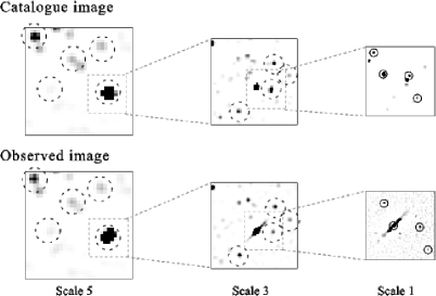
Figure 3: Wavelet transform of the reference image (simulated image from a catalog), and the wavelet transform of the input image to be registered. The circles show some associations done with the window search scale by scale. Only a part of the wavelet planes are shown via a zoom from one scale to a lower one, in order to improve the visibility. Scale 5 is the last scale (lowest-resolution) of the wavelet transform. A rough distortion model is deduced from this scale. It is then refined with the other scale up to scale 1. The final distortion model is made with a second order polynomial.

The advantage of the multi-resolution approach is that it is insensitive to the presence of spurious objects in the reference catalog (stars with large proper motion, objects that do not appear on the observed image due to their color). This multi-resolution approach has also proven to be very efficient in very crowded areas such as the Small Magellanic Cloud. Exhaustive tests have also been performed on images of the open cluster Messier 67 observed with wide-field imager [9].

5.3 Satellite track detection

A frequent problem encountered in imaging surveys using wide-field imagers is the presence of a significant number of satellite tracks. This is a non-trivial problem for survey work since these features, if not identified in the original exposures, will appear in the final co-added image. The presence of these tracks are not only unpleasant from the cosmetic point of view but also have a considerable impact on the derived products (source extraction). Once propagated to the final image, none of the available options are adequate. One can either mask the final image, which may continue to affect the source extraction, or to go back to the individual exposures, mask the visible tracks, and stack the images again. While this manual process can be done for a few images it is certainly not feasible for large data flows given the high incidence of these features. Therefore, a robust system must be able to identify and remove these unwanted features automatically during the processing phase which precedes the stacking [11].

Fortunately, this problem can be tackled using the Fast Hough Transform (FHT) [7] since a track consists of a set of points aligned in an otherwise quasi-random distribution of points. The method is based on the fact that the FHT transforms points to the original space into lines (using Bresenham’s procedure) in the Hough space. In this space the intersection of the lines correspond to the parameters of a straight line in the original space.

The Hough space is a two-dimensional space in which each point $x,y$ in the image space is transformed into a line given by $y=-x*X+y$. The amplitude in the Hough space is the sum of the number of points contributing at each position in this space. The alignement of $N$ points in real space following the relatiion $y_{i}=a*x_{i}+b$, where $i=1,N$, will imply a peak in the intensity of the amplitude in Hough space at the point ($X=a,Y=b$) given by $b=-x_{i}*a+y_{i}$. This transformation is illustrated in Figure 4 where two tracks in real space are shown in the left panel and the Hough transform of all points along these two lines are represented in the Hough space in the right panel. As discussed above the intersection of the point-transformed leads to an intersection in the Hough space yielding a local maximum. The identification of these high-amplitude peaks yields the coefficients $a$ and $b$ that correspond to the slope and the offset of the track in real space.

Note, however, that the case shown is valid only for slopes in the interval $[-1,+1]$. In order to deal with slopes outside this range and limit the size of the FHT space, the original catalog is flipped to satisfy the same conditions. Therefore, the actual implementation of the algorithm consists of two steps.

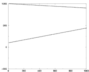
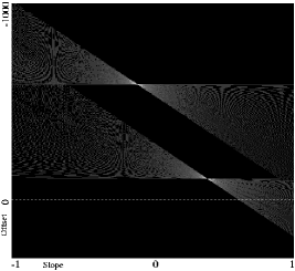
Figure 4: Example of the FHT of two sets of aligned points.

Using the method described above a catalog is extracted from single exposures considering significant local maxima. This catalog is FHTed, and a high-pass filter is used to remove the constant response of FHT. Finally, possible tracks are identified on the Hough filtered image applying a fixed threshold given by $\frac{\sqrt{N}}{k}$, where $N$ is the number of points in catalog, and, $k$ is the sensitivity factor. Tests show that $k=2$ is adequate for very faint detections without false positives. To illustrate the method Figure 5 shows a portion of an image with a faint satellite track (left panel), where the dashed line represents the line detected by the procedure on the Hough filtered image (right panel). This methodology has now been implemented in the EIS pipeline and it is routinely used with very good results.

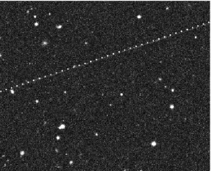
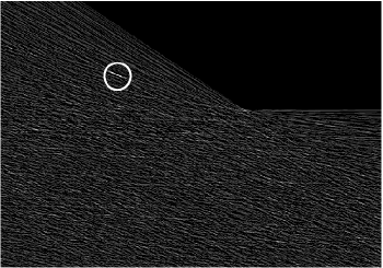
Figure 5: Detected track in Hough Space, displayed as a dotted line in the original image.

6 General Comments about the code and Performance

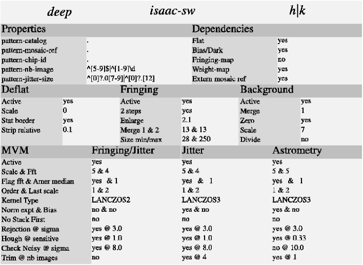
Figure 6: An illustration of an HTML page created from the XML log produced by the system. It displays the main parameters which define the Reduction Mode used for the IR camera ISAAC, mounted on one of the ESO VLT telescopes. The reduction mode shown is used for processing images observed with the filters H or K. The field properties, for instance, lists the minimum number of images in the RB and the minimum amplitude of the jitter pattern required for the execution of this RM. Dependencies lists the master calibration images needed for reduction. In this example all steps of the reduction mode are active, namely: instrumental effect removal; local background estimation using masks; removal of low-frequency background; and stacking using relative astrometry, followed by an absolute registration of the stacked image using a reference grid specified in the section dependencies. Also shown are possible settings for the various sub-processes such as: noisy image rejection, cosmic rays removal and track detection using Hough transform.

The software package presented here is an evolution of the so called multi-resolution visual model or MVM, which consists of basic functions for operations on images, wavelet transform and image registration, complemented by open source libraries such as CFITSIO, FFTW and LIBXML2, among others. The MVM library is written in C++ and runs on different platforms: SUN-OS, TRUE-64 on an ALPHA computer, and PC-Linux. Using these basic blocks the package described in this paper has been developed over the past two years to deal with the specific needs of astronomical images and consists of 90.000 lines of code. The various processes are bound together by employing the Extensible Mark-up Language (XML) technology which is used to input parameters, as a way of communicating between different modules, as an internal database and to store the history of the process. The latter can be much more comprehensive than it would be possible in the FITS header of the image. Furthermore, the associated XML files can be translated to any format and make their content available in a human-readable form using suitable style-sheets (XSLT protocol), which can be processed to produce and display HTML pages. An example is shown in figure 6 where the parameters characterizing a particular reduction mode are shown. The figure illustrates the use of a particular style-sheet which produces a concise description for internal use. A more comprehensive style-sheet is used for other users, which gives more detailed information about each parameter.

By using a common library approach, instead of a concatenation of stand-alone programs, the package avoids unnecessary access to disk and the entire reduction is carried out in memory, thereby enhancing significantly the data rate of the process. This is paramount for dealing with large data volumes, and is true both for the stand-alone implementation and the plug-in version for the survey system. In the latter case, the Python wrapper is only responsible for the preparation and the administration of the RBs, thereafter launching the reduction process. The communication between Python and the library is only done at the beginning and at the end of the process via the XML configuration and log files produced.

The stand-alone version of the package has been extensively used to reduce images from a variety of past and ongoing public surveys allowing thus a fairly robust estimate of its performance. Some examples are given in Table 1, where the survey name, type, instrument, detector size, number of images and total time required for the reduction are listed.

Survey name	Type of survey	Instrument	Detector Size	# sci images	CPU time
CDF South [1]	deep optical	WFI @ 2.2	8 x 2k x 4k	246	9 h
CDF South [12]	deep IR	SOFI @ NTT	1 x 1k x 1k	4300	3h
Pre Flame survey [9]	stellar optical	WFI @ 2.2	8 x 2k x 4k	26	1h
GOOD survey [5]	deep IR	ISAAC @ VLT	1 x 1k x 1k	6000	4h

Table 1: Examples of the performance of the system.

The performance refers to an Alpha DS20E running at 666 MHz with two CPUs. The values listed above yield a typical reduction data-rate of $0.5$ Mega-pixels per second for optical images, and $0.4$ Mega-pixels per second for IR images (which requires the removal of fringes). The overhead time for the preparation and the reduction of the calibration images depends on the instrument, and it is typically $50$ percent of the reduction time. The pipeline has also been tested successfully on other multi-CCD instruments such as: the CFHT 12k camera, and the SUSI2 instrument mounted on the ESO-NTT telescope.

7 Conclusion

In this paper a new image reduction system, incorporating new technologies and algorithms is presented. It is part of the effort of the EIS team at ESO to develop an integrated, end-to-end survey system capable of converting raw images to science-grade products from multi-wavelength, multi-instrument public surveys. The system incorporates a number of procedures design to cope with a variety of particular situations encountered in real observations covering the optical/infrared domain. The system has a high-throughput ($\sim$ 0.5 Mega-pixels/sec) and handles the entire suite of imagers available at ESO. It also makes extensive use of XML technology to interface with the user and to provide the full history of the process. The code is written in C++ and it is platform independent. The development of new algorithms is still ongoing (e.g., illumination correction) as well as work aiming at the full integration of the library into the survey system. Efforts are also made to prepare the required documentation and user interface to make the stand-alone version of the image reduction pipeline publicly available.

- [1] S. Arnouts, B. Vandame, C. Benoist, M. A. T. Groenewegen, L. da Costa, M. Schirmer, R. P. Mignani, R. Slijkhuis, E. Hatziminaoglou, R. Hook, R. Madejsky, C. Rité, and A. Wicenec. ESO imaging survey. Deep public survey: Multi-color optical data for the Chandra Deep Field South. A&A, 379:740–754, November 2001.
- [2] E. Bertin. SWarp User Guide v1.34. http://terapix.iap.fr/soft/swarp/, 2002.
- [3] L. da Costa. Public Imaging Surveys: Survey Systems and Scientific Opportunities. In Mining the Sky, pages 521–+, 2001.
- [4] J.P. Djandji, A. Bijaoui, and R. Mamère. Geometrical Registration of images. The multiresolution approach. Photogrammetric Engineering and Remote Sensing, (59):645–653, 1993.
- [5] R. Fosbury, J. Bergeron, C. Cesarsky, S. Cristiani, R. Hook, A. Renzini, and P. Rosati. The Great Observatories Origins Deep Survey (GOODS). The Messenger, 105:40–+, September 2001.
- [6] M. A. T. Groenewegen, S. Arnouts, C. Benoist, L. da Costa, M. Schirmer, R. P. Mignani, R. Slijkhuis, E. Hatziminaoglou, R. Hook, R. Madejsky, C. Rité, B. Vandame, and A. Wicenec. ESO imaging survey. The stellar catalogue in the Chandra deep field south. A&A, 2002.
- [7] Hough. 1962.
- [8] S. Mallat. A Theory for Multiresolution Signal Decomposition the wavelet representation. IEEE, 11(7):674–693, 1989.
- [9] Y. Momany, B. Vandame, S. Zaggia, R. P. Mignani, L. da Costa, S. Arnouts, M. A. T. Groenewegen, E. Hatziminaoglou, R. Madejsky, C. Rité, M. Schirmer, and R. Slijkhuis. ESO imaging survey. Pre-FLAMES survey: Observations of selected stellar fields. A&A, 379:436–452, November 2001.
- [10] A. Renzini and L. N. da Costa. The ESO Imaging Survey. The Messenger, 87:23–26, 1997.
- [11] B. Vandame. Fast Hough Transform for Robust Detection of Satellite Tracks. In Mining the Sky, pages 595–+, 2001.
- [12] B. Vandame, S. Arnouts, C. Benoist, M. A. T. Groenewegen, L. da Costa, M. Schirmer, R. P. Mignani, R. Slijkhuis, E. Hatziminaoglou, R. Hook, R. Madejsky, C. Rité, and A. Wicenec. ESO Imaging Survey. Deep Public Survey: Infrared Data for the Chandra Deep Field South. A&A, 2002 under revision.