OVRO CMB Anisotropy Measurement Constraints on Flat- $\Lambda$ and Open CDM Cosmogonies

Pia Mukherjee¹¹affiliation: Department of Physics, Kansas State University, 116 Cardwell Hall, Manhattan, KS 66506. , Tarun Souradeep¹¹affiliation: Department of Physics, Kansas State University, 116 Cardwell Hall, Manhattan, KS 66506. ²²affiliation: Current address: IUCAA, Post Bag 4, Ganeshkhind, Pune 411007, India. , Bharat Ratra¹¹affiliation: Department of Physics, Kansas State University, 116 Cardwell Hall, Manhattan, KS 66506. , Naoshi Sugiyama³³affiliation: Division of Theoretical Astrophysics, National Astronomical Observatory, 2-21-1 Osawa, Mitaka, Tokyo 181-8588, Japan. ⁴⁴affiliation: Max Planck Institute for Astrophysics, Karl-Schwarzschild Str. 1, Postfach 1317, Garching D-85741, Germany. , and Krzysztof M. Górski⁵⁵affiliation: European Southern Observatory, Karl-Schwarzschild Str. 2, Garching D-85748, Germany. ⁶⁶affiliation: Warsaw University Observatory, Aleje Ujazdowskie 4, 00-478 Warszawa, Poland.

Abstract

We use Owens Valley Radio Observatory (OVRO) cosmic microwave background (CMB) anisotropy data to constrain cosmological parameters. We account for the OVRO beamwidth and calibration uncertainties, as well as the uncertainty induced by the removal of non-CMB foreground contamination. We consider open and spatially-flat- $\Lambda$ cold dark matter cosmogonies, with nonrelativistic-mass density parameter $\Omega_{0}$ in the range 0.1–1, baryonic-mass density parameter $\Omega_{B}$ in the range (0.005–0.029) $h^{-2}$ , and age of the universe $t_{0}$ in the range (10–20) Gyr. Marginalizing over all parameters but $\Omega_{0}$ , the OVRO data favors an open (spatially-flat- $\Lambda$ ) model with $\Omega_{0}\simeq$ 0.33 (0.1). At the 2 $\sigma$ confidence level model normalizations deduced from the OVRO data are mostly consistent with those deduced from the DMR, UCSB South Pole 1994, Python I-III, ARGO, MAX 4 and 5, White Dish, and SuZIE data sets.

cosmic microwave background—cosmology: observations—large-scale structure of the universe

^†^†slugcomment: KSUPT-02/4 August 2002

1 Introduction

Cosmic microwave background (CMB) anisotropy measurements have begun to provide interesting constraints on cosmological parameters.¹¹1 See, e.g., Miller et al. (2002a), Coble et al. (2001), Scott et al. (2002), and Mason et al. (2002) for recent measurements, and, e.g., Podariu et al. (2001), Wang, Tegmark, & Zaldarriaga (2002), Durrer, Novosyadlyj, & Apunevych (2001), and Miller et al. (2002b) for recent discussions of constraints on cosmological parameters. Ganga et al. (1997a, hereafter GRGS) developed a technique to account for uncertainties, such as those in the beamwidth and the calibration, in likelihood analyses of CMB anisotropy data. This technique has been used with theoretically-predicted CMB anisotropy spectra in analyses of the Gundersen et al. (1995) UCSB South Pole 1994 data, the Church et al. (1997) SuZIE data, the Lim et al. (1996) MAX 4+5 data, the Tucker et al. (1993) White Dish data, the de Bernardis et al. (1994) ARGO data, and the Platt et al. (1997) Python I-III data (GRGS; Ganga et al. 1997b, 1998; Ratra et al. 1998, 1999a, hereafter R99a; Rocha et al. 1999, hereafter R99). A combined analysis of all these data sets, excluding the Python data, is presented in Ratra et al. (1999b, hereafter R99b).

In this paper we present a similar analysis of CMB anisotropy data from the OVRO observations (Leitch et al. 2000, hereafter L00). The OVRO detectors and telescopes are described in Leitch (1998) and L00; here we review information about the experiment that is needed for our analysis.

OVRO data were taken in two frequency bands, one centered at 14.5 GHz (Ku band), the other at 31.7 GHz (Ka band). Thirty-six fields, along an approximate circle at declination $\delta\simeq 88^{\circ}$ centered on the North Celestial Pole (NCP) were observed. In our computations we use the coordinates for the 36 fields given in Table 2 of L00. The OVRO measurements were made by switching the beam in a two-point pattern along the circle, resulting in a three-beam response to the sky signal. The beamthrow is $22^{\prime}{\!}.16$ . The zero-lag window function parameters for the OVRO experiment are given in Table 1. This and other window functions are shown in Fig. 18 of L00.

L00 use multiepoch VLA observations to detect and remove non-CMB discrete source contamination from the OVRO data. We have also analyzed the OVRO data ignoring 3 of the 36 fields that were affected by the strongest variable discrete source; cosmological constraints derived from this restricted OVRO CMB anisotropy data set are very consistent with those derived from the full OVRO CMB anisotropy data set, so we do not discuss this restricted OVRO data set analysis further.

Since OVRO data were taken at two frequencies, it is possible to fit the data to both a non-CMB foreground component (parametrized by the frequency dependent temperature anisotropy $\Delta T_{\rm fore}\propto\nu^{\beta}$ ) and a CMB anisotropy component with spectral index $\beta=0$ .²²2 See L00 and Mukherjee et al. (2002) for discussions of foreground contaminants in the OVRO microwave data. We use the method in $\S$ 11 of L00 to extract the CMB anisotropy component in the OVRO data, marginalizing over a foreground spectral index in the range $-3<\beta<2$ in our likelihood analysis.³³3 Although the data themselves are unable to rule out more negative values of beta (L00, Fig. 14), Leitch et al. (1997) use low frequency maps of the NCP region to rule out such values.^,⁴⁴4 Following Mukherjee et al. (2002) we have also analyzed the 31.7 GHz OVRO CMB anisotropy data while marginalizing over possible 100 $\mu$ m and 12 $\mu$ m foreground contaminant template (Schlegel, Finkbeiner, & Davis 1998) correlated components. The cosmological constraints from these analyzes are quite consistent with results presented here. This is because although the foreground signal inferred in our analysis is not entirely fit by the dust data, they are significantly correlated, and the 31.7 GHz data, modelled either way, is almost entirely CMB anisotropy. The OVRO data at its two frequencies are shown in Fig. 13 of L00, the deduced CMB anisotropy and foreground signals are shown in Fig. 16 of L00, and the dust-correlated emission is shown in Fig. 1 of Mukherjee et al. (2002).

CMB anisotropy constraints are derived from the foreground-corrected 31.7 GHz data.⁵⁵5 At $\beta=-2.2$ for the foreground contaminant, $96\%$ of the 31.7 GHz data is CMB anisotropy. The 31.7 GHz beam profile is well approximated by a circular Gaussian of FWHM $7^{\prime}{\!}.37\pm 0^{\prime}{\!}.26$ (one standard deviation uncertainty). We use the method of GRGS to account for the OVRO beam uncertainty.

As discussed in L00, the noise in the 31.7 GHz data indicates the presence of a component that is correlated between neighboring fields (this component is small compared to the uncorrelated noise in a single scan of data). As a result the 31.7 GHz OVRO data show only one-half of the anticorrelation for nearest neighbor fields expected for a triple beam chopped experiment.⁶⁶6 Models that neglect these correlations are grossly discrepant with the data, while when these correlations are accounted for the model fits are reasonable and consistent with the data. This can be seen from Fig. 19 of L00 and we find the same. This one-offdiagonal correlated noise is included and its amplitude marginalized over in our analysis.

A constant offset is removed from the OVRO data; we marginalize over the amplitude of the offset to account for this in our likelihood analysis. The 1 $\sigma$ absolute calibration uncertainty of the OVRO data is $4.3\%$ , and the method developed by GRGS is used to account for it.

In $\S$ 2 we summarize the computational techniques used in our analysis. See GRGS and R99a for detailed discussions. Results are presented and discussed in $\S$ 3. We conclude in $\S$ 4.

2 Summary of Computation

In this paper we focus on a spatially-flat CDM model with a cosmological constant $\Lambda$ .⁷⁷7 See, e.g., Peebles (1984), Efstathiou, Sutherland, & Maddox (1990), Stompor, Górski, & Banday (1995), Ratra et al. (1997), Sahni & Starobinsky (2000), Carroll (2001), and Peebles & Ratra (2002). While not considered in this paper, a time-variable dark energy dominated spatially-flat model is also largely consistent with current observations (see, e.g., Peebles & Ratra 1988; Ratra & Quillen 1992; Steinhardt 1999; Brax, Martin, & Riazuelo 2000; Huterer & Turner 2001; Chen & Ratra 2002; Deustua et al. 2002). As a foil we also consider a spatially open model with no $\Lambda$ (see, e.g., Gott 1982; Ratra & Peebles 1995). These models are discussed in more detail in R99a, R99b, and R99.

The CMB anisotropy spectra in these models are generated from quantum fluctuations in weakly coupled fields during an early epoch of inflation and so are Gausssian (see, e.g., Ratra 1985; Fischler, Ratra, & Susskind 1985). Consistent with this, the observed smaller-scale CMB anisotropy appears to be Gaussian (see, e.g., Park et al. 2001, Wu et al. 2001; Shandarin et al. 2002; Polenta et al. 2002), and the experimental noise also appears to be Gaussian, thus validating our use of the GRGS likelihood analysis method.

As discussed in R99a, the spectra are parameterized by their quadrupole-moment amplitude $Q_{\rm rms-PS}$ , the nonrelativistic-mass density parameter $\Omega_{0}$ , the baryonic-mass density parameter $\Omega_{B}$ , and the age of the universe $t_{0}$ . The spectra are computed for a range of $\Omega_{0}$ spanning the interval 0.1 to 1 in steps of 0.1, for a range of $\Omega_{B}h^{2}$ [the Hubble parameter $h=H_{0}/(100\ {\rm km}\ {\rm s}^{-1}\ {\rm Mpc}^{-1})$ ] spanning the interval 0.005 to 0.029 in steps of 0.004, and for a range of $t_{0}$ spanning the interval 10 to 20 Gyr in steps of 2 Gyr. In total 798 spectra were computed to cover the cosmological-parameter spaces of the open and flat- $\Lambda$ models. Examples of spectra are shown in Fig. 2 of R99a, Fig. 1 of R99b, and Fig. 2 of R99.

Following GRGS, for each of the 798 spectra considered the “bare” likelihood function is computed at the nominal beamwidth and calibration, as well as at a number of other values of the beamwidth and calibration determined from the measurement uncertainties. The likelihood function used in the derivation of the central values and limits is determined by integrating (marginalizing) the bare likelihood function over the beamwidth and calibration uncertainties with weights determined by the measured probability distribution functions of the beamwidth and the calibration. See GRGS for a more detailed discussion. The likelihoods are a function of four parameters mentioned above: $Q_{\rm rms-PS}$ , $\Omega_{0}$ , $\Omega_{B}h^{2}$ , and $t_{0}$ . We also compute marginalized likelihood functions by integrating over one or more of these parameters after assuming a uniform prior in the relevant parameters. The prior is set to zero outside the ranges considered for the parameters. GRGS and R99a describe the prescription used to determine central values and limits from the likelihood functions. In what follows we consider 1, 2, and 3 $\sigma$ highest posterior density limits which include 68.3, 95.4, and 99.7% of the area.

3 Results and Discussion

Table 2 lists the derived values of $Q_{\rm rms-PS}$ and bandtemperature $\delta T_{l}$ for the flat bandpower spectrum, for the OVRO data. These numerical values account for the correlated noise and offset removal, the beamwidth and calibration uncertainties, and the uncertainty due to non-CMB diffuse foreground contamination removal. These results are very consistent with those of L00. For the flat bandpower spectrum the OVRO data average 1 $\sigma$ $\delta T_{l}$ error bar is $\sim 14\%$ ⁸⁸8 For comparison, the corresponding 1 $\sigma$ $\delta T_{l}$ error bar is $\sim 10-12\%$ for DMR (depending on model, Górski et al. 1998), $\sim 15\%$ for ARGO (R99a), and $\sim 14\%$ for MAX 4+5 (Ganga et al. 1998). : OVRO data results in a very significant detection of CMB anisotropy, even after accounting for the uncertainties listed above.

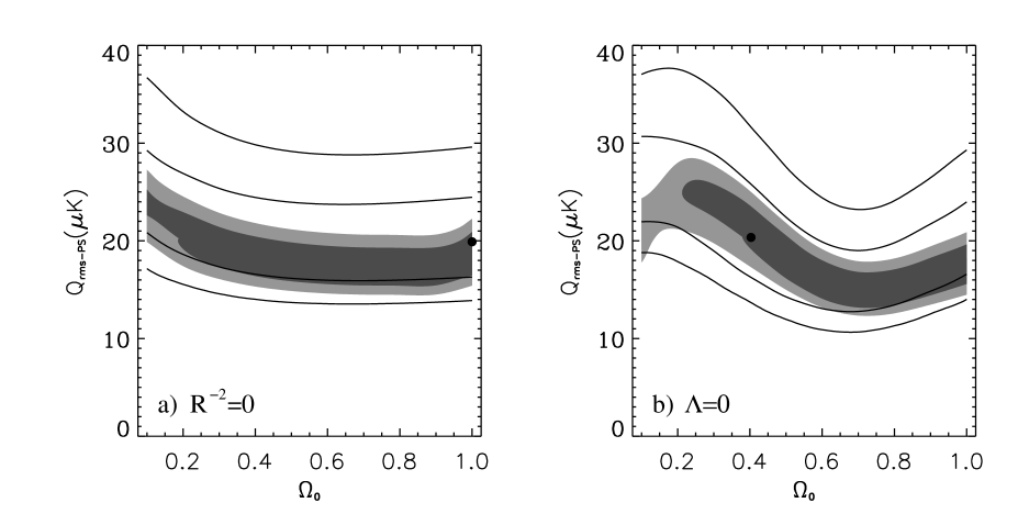
As discussed in R99a, R99b, and R99, the four-dimensional posterior probability density distribution function $L(Q_{\rm rms-PS},\Omega_{0},\Omega_{B}h^{2},t_{0})$ is nicely peaked in the $Q_{\rm rms-PS}$ direction but fairly flat in the other three directions. Marginalizing over $Q_{\rm rms-PS}$ results in a three-dimensional posterior distribution $L(\Omega_{0},\Omega_{B}h^{2},t_{0})$ which is steeper, but still relatively flat. As a consequence, limits derived from the four- and three-dimensional posterior distributions are generally not highly statistically significant. We therefore do not show contour plots of these functions here. Marginalizing over $Q_{\rm rms-PS}$ and one other parameter results in two-dimensional posterior probability distributions which are more peaked (see Figs. 1). As in the ARGO (R99a), Python (R99), and combination (R99b) data set analyses, in some cases these peaks are at an edge of the parameter range considered.

Figure 1 shows that the two-dimensional posterior distributions allow one to distinguish between different regions of parameter space at a fairly high formal level of confidence.⁹⁹9 See Fig. 4 of R99a, Fig. 2 of R99b, and Fig. 3 of R99 for related cosmological constraints from other data. For instance, the open model near $\Omega_{0}\sim 0.75$ , $\Omega_{B}h^{2}\sim 0.03$ , and $t_{0}\sim 20$ Gyr, and the flat- $\Lambda$ model near $\Omega_{0}\sim 0.6$ , $\Omega_{B}h^{2}\sim 0.03$ , and $t_{0}\sim 20$ Gyr, are both formally ruled out at $\sim 3$ $\sigma$ confidence. However, we emphasize, as discussed in R99a, R99b, and R99, care must be exercised when interpreting the discriminative power of these formal limits, since they depend sensitively on the fact that the uniform prior has been set to zero outside the range of the parameter space we have considered.

Figure 2 shows the contours of the two-dimensional posterior distribution for $Q_{\rm rms-PS}$ and $\Omega_{0}$ , derived by marginalizing the four-dimensional distribution over $\Omega_{B}h^{2}$ and $t_{0}$ . These are shown for the OVRO and DMR data, for both the open and flat- $\Lambda$ models. Constraints on these parameters from the OVRO data are consistent with those from the DMR data.

Figure 3 shows the one-dimensional posterior distribution functions for $\Omega_{0}$ , $\Omega_{B}h^{2}$ , $t_{0}$ , and $Q_{\rm rms-PS}$ , derived by marginalizing the four-dimensional posterior distribution over the other three parameters. From these one-dimensional distributions, the OVRO data favors an open (flat- $\Lambda$ ) model with $\Omega_{0}$ = 0.33 (0.10), or $\Omega_{B}h^{2}$ = 0.005 (0.005), or $t_{0}$ = 10 (11) Gyr, amongst the models considered. At 2 $\sigma$ confidence the OVRO data formally rule out only small regions of parameter space. From the one-dimensional distributions of Fig. 3, the data require $\Omega_{0}$ $<0.69$ or $>0.75$ ( $\Omega_{0}$ $<0.51$ or $>0.56$ ), or $\Omega_{B}h^{2}$ $<0.028$ ( $\Omega_{B}h^{2}$ $<0.028$ ), or $t_{0}$ $<19$ Gyr ( $t_{0}$ $<19$ Gyr) for the open (flat- $\Lambda$ ) model at 2 $\sigma$ .

While the statistical significance of the constraints on cosmological parameters is not high, it is reassuring that the OVRO data favor low-density, young models, consistent with indications from most other data. The constraints on $\Omega_{B}h^{2}$ derived from the OVRO data are somewhat puzzling. They are more consistent with those derived from the Python and combination CMB anisotropy data sets analyzed by R99 and R99b, but less so with those from ARGO (R99a) and more recent data sets (Netterfield et al. 2002; Pryke et al. 2002; Stompor et al. 2001) which favor higher $\Omega_{B}h^{2}$ . The lower $\Omega_{B}h^{2}$ found here is more consistent with the low Cyburt, Fields, & Olive (2001) standard nucleosynthesis value determined from helium and lithium abundance measurements, and less consistent with the high deuterium-based value of Burles, Nollett, & Turner (2001).

The peak values of the one-dimensional posterior distributions shown in Fig. 3 are listed in the figure caption for the case when the four-dimensional posterior distributions are normalized such that $L(Q_{\rm rms-PS}\ =\ 0\ \mu{\rm K})\ =\ 1$ . With this normalization, marginalizing over the remaining parameter the fully marginalized posterior distributions are $1.4\times 10^{67}(1.3\times 10^{67})$ for the open (flat- $\Lambda$ ) model. This is not inconsistent with the indication from panels $a)$ and $b)$ of Fig. 3 that the most-favored open model is marginally more favored than the most-favored flat- $\Lambda$ one.

4 Conclusion

The OVRO data results derived here are mostly consistent with those derived from the DMR, SP94, Python I-III, ARGO, MAX 4+5, White Dish and SuZIE data. The OVRO data significantly constrains $Q_{\rm rms-PS}$ (for the flat bandpower spectrum $Q_{\rm rms-PS}\ =\ 38{+6\atop-5}\ \mu$ K at 1 $\sigma$ ) and weakly favors low-density, low $\Omega_{B}h^{2}$ , young models.

We acknowledge valuable assistance from R. Stompor and helpful discussions with K. Ganga and E. Leitch. PM, BR, and TS acknowledge support from NSF CAREER grant AST-9875031. NS acknowledges support from the Alexander von Humboldt Foundation and Japanese Grant-in-Aid for Science Research Fund No. 14540290.

Table 1: Numerical Values for the Zero-Lag Window Function Parameters^a^aThe value of

l

where

W_{l}

is largest,

l_{\rm m}

, the two values of

l

where

W_{l_{e^{-0.5}}}=e^{-0.5}W_{l_{\rm m}}

l_{e^{-0.5}}

, the effective multipole,

l_{\rm e}=I(lW_{l})/I(W_{l})

, and

I(W_{l})=\sum^{\infty}_{l=2}(l+0.5)W_{l}/\{l(l+1)\}

$l_{e^{-0.5}}$	$l_{\rm e}$	$l_{\rm m}$	$l_{e^{-0.5}}$	$\sqrt{I(W_{l})}$
360	596	537	753	1.41

Table 2: Numerical Values for

Q_{\rm rms-PS}

and

\delta T_{l}

from Likelihood Analyses Assuming a Flat Bandpower Spectrum

$Q_{\rm rms-PS}$ ^a^aThe first of the three entries is where the posterior probability density distribution function peaks and the vertical pair of numbers are the $\pm 1$ $\sigma$ (68.3% highest posterior density) values.	Ave. Abs. Err.^b^bAverage absolute error on $Q_{\rm rms-PS}$ in $\mu$ K.	Ave. Frac. Err.^c^cAverage fractional error, as a fraction of the central value.	$\delta T_{l}$ ^a^afootnotemark:	LR^d^dLikelihood ratio.
( $\mu$ K)	( $\mu$ K)		( $\mu$ K)
38 ${44\atop 33}$	5.5	14%	59 ${69\atop 51}$	$9\times 10^{66}$

References

Brax, Martin, & Riazuelo (2000) Brax, P., Martin, J., & Riazuelo, A. 2000, Phys. Rev. D, 62, 103505
Burles et al. (2001) Burles, S., Nollett, K. M., & Turner, M. S. 2001, ApJ, 552, L1
Carroll (2001) Carroll, S.M. 2001, Living Rev. Relativity, 4, 1
Chen & Ratra (2002) Chen, G., & Ratra, B. 2002, astro-ph/0207051
Church et al. (1997) Church, S. E., Ganga, K. M., Ade, P. A. R., Holzapfel, W. L., Mauskopf, P. D., Wilbanks, T. M., & Lange, A. E. 1997, ApJ, 484, 523
Coble et al. (2001) Coble, K., Dodelson, S., Dragovan, M., Ganga, K., Knox, L., Kovac, J., Ratra, B., & Souradeep, T. 2001, astro-ph/0112506
Cyburt et al. (2001) Cyburt, R. H., Fields, B. D., & Olive, K. A. 2001, New Astron., 6, 215.
de Bernardis et al. (1994) de Bernardis, P., et al. 1994, ApJ, 422, L33
Deustua et al. (2002) Deustua, S., Caldwell, R., Garnavich, P., Hui, L., & Refregier, A. 2002, astro-ph/0207293
Durrer et al (2001) Durrer, R., Novosyadlyj, B., & Apunevych, S. 2001, astro-ph/0111594
Efstathiou et al. (1990) Efstathiou, G., Sutherland, W. J., & Maddox, S. J. 1990, Nature, 348, 705
Fischler et al. (1985) Fischler, W., Ratra, B., & Susskind, L. 1985, Nucl. Phys. B, 259, 730.
Ganga et al. (1997b) Ganga, K., Ratra, B., Church, S. E., Sugiyama, N., Ade, P. A. R., Holzapfel, W. L., Mauskopf, P.D., & Lange, A. E. 1997b, ApJ, 484, 517
Ganga et al. (1997a) Ganga, K., Ratra, B., Gundersen, J. O., & Sugiyama, N. 1997a, ApJ, 484, 7 (GRGS)
Ganga et al. (1998) Ganga, K., Ratra, B., Lim, M. A., Sugiyama, N., & Tanaka, S. T. 1998, ApJS, 114, 165
Gorski et al. (1998) Górski, K. M., Ratra, B., Stompor, R., Sugiyama, N., & Banday, A. J. 1998, ApJS, 114, 1
Gott (1982) Gott, J.R. 1982, Nature, 295, 304
Gundersen et al. (1995) Gundersen, J. O., et al. 1995, ApJ, 443, L57
Huterer & Turner (2001) Huterer, D., & Turner, M. S. 2001, Phys. Rev. D, 64, 123527
Leitch (1998) Leitch, E. M. 1998, PhD thesis, California Institute of Technology
Leitch et al. (1997) Leitch, E. M., Readhead, A. C. S., Pearson, T. J., & Myers, S. T. 1997, ApJ, 486, L23
Leitch et al. (2000) Leitch, E. M., Readhead, A. C. S., Pearson, T. J., Myers, S. T., Gulkis, S., & Lawrence C. R. 2000, ApJ, 532, 37 (L00)
Lim et al. (1996) Lim, M. A., et al. 1996, ApJ, 469, L69
Mason et al. (2002) Mason, B. S., et al. 2002, astro-ph/0205384
Miller et al. (2002a) Miller, A. D., et al. 2002a, ApJS, 140, 115
Miller et al. (2002b) Miller, C. J., Nichol, R. C., Genovese, C., & Wasserman, L. 2002b, ApJ, 565, L67
Mukherjee et al. (2002) Mukherjee, P., Dennison, B., Ratra, B., Simonetti, J. H., Ganga, K., & Hamilton, J.-Ch. 2002, ApJ (in press), astro-ph/0110457
Netterfield et al. (2002) Netterfield, C. B., et al. 2002, ApJ, 571, 604
Park et al. (2001) Park, C.-G., Park, C., Ratra, B., & Tegmark, M. 2001, ApJ, 556, 582
Peebles (1984) Peebles, P. J. E. 1984, ApJ, 284, 439
Peebles & Ratra (1988) Peebles, P. J. E., & Ratra, B. 1988, ApJ, 325, L17
Peebles & Ratra (2002) Peebles, P. J. E., & Ratra, B. 2002, astro-ph/0207347
Platt et al. (1997) Platt, S. R., Kovac, J., Dragovan, M., Peterson, J. B., & Ruhl, J. E. 1997, ApJ, 475, L1
Podariu et al. (2001) Podariu, S., Souradeep, T., Gott, J. R., Ratra, B., & Vogeley, M. S. 2001, ApJ, 559, 9
Polenta et al. (2002) Polenta, G., et al., 2002, ApJ, 572, L27
Pryke et al (2002) Pryke, C., Halverson, N. W., Leitch, E. M., Kovac, J., Carlstrom, J. E., Holzapfel, W. L., & Dragovan, M. 2002, ApJ, 568, 46
Ratra (1985) Ratra, B. 1985, Phys. Rev. D, 31, 1931
Ratra et al. (1999a) Ratra, B., Ganga, K., Stompor, R., Sugiyama, N., de Bernardis, P., & Górski, K. M. 1999a, ApJ, 510, 11 (R99a)
Ratra et al. (1998) Ratra, B., Ganga, K., Sugiyama, N., Tucker, G. S., Griffin, G. S., Nguyên, H. T., & Peterson, J. B. 1998, ApJ, 505, 8
Ratra & Peebles (1995) Ratra, B., & Peebles, P. J. E. 1995, Phys. Rev. D, 52, 1837
Ratra & Quillen (1992) Ratra, B., & Quillen, A. 1992, MNRAS, 259, 738
Ratra et al. (1999b) Ratra, B., Stompor, R., Ganga, K., Rocha, G., Sugiyama, N., & Górski, K. M. 1999b, ApJ, 517, 549 (R99b)
Ratra et al. (1997) Ratra, B., Sugiyama, N., Banday, A. J., & Górski, K. M. 1997, ApJ, 481, 22
Rocha et al. (1999) Rocha, G., Stompor, R., Ganga, K., Ratra, B., Platt, S. R., Sugiyama, N., & Górski, K. M. 1999, ApJ, 525, 1 (R99)
Sahni & Starobinsky (2000) Sahni, V., & Starobinsky, A. 2000, Int. J. Mod. Phys. D, 9, 373
Schlegel et al. (1998) Schlegel, D. J., Finkbeiner, D. P., & Davis, M. 1998, ApJ, 500, 525
Scott et al. (2002) Scott, P. F., et al. 2002, astro-ph/0205380
Shandarin et al. (2002) Shandarin, S. F., Feldman, H. A., Xu, Y., & Tegmark, M. 2002, ApJS, 141, 1
Steinhardt (1999) Steinhardt, P.J. 1999, in Proceedings of the Pritzker Symposium on the Status of Inflationary Cosmology, in press
Stompor (1997) Stompor, R. 1997, in Microwave Background Anisotropies, ed. F. R. Bouchet, R. Gispert, B. Guiderdoni, & J. Tran Thanh Van (Gif-sur-Yvette: Editions Frontieres), 91
Stompor et al. (2001) Stompor, R., et al. 2001, ApJ, 561, L7
Stompor et al. (1995) Stompor, R., Górski, K. M., & Banday, A. J. 1995, MNRAS, 277, 1225
Tucker et al. (1993) Tucker, G. S., Griffin, G. S., Nguyên, H. T., & Peterson, J. B. 1993, ApJ, 419, L45
Wang et al. (2002) Wang, X., Tegmark, M., & Zaldarriaga, M. 2002, Phys. Rev. D, 65, 123001
Wu et al. (2001) Wu, J.-H. P., et al. 2001, Phys. Rev. Lett., 87, 251303

Refer to caption — Figure 1: Confidence contours and maxima of the OVRO data two-dimensional posterior probability density distribution functions, as a function of the two parameters on the axes of each panel (derived by marginalizing the four-dimensional posterior distributions over the other two parameters). Dashed lines (crosses) show the contours (maxima) of the open case and solid lines (solid circles) show those of the flat- $\Lambda$ model. Panel $a)$ shows the $(\Omega_{B}h^{2},\ \Omega_{0})$ plane, and panel $b)$ shows the $(t_{0},\ \Omega_{0})$ plane.