Magnetic field strengths in the hotspots and lobes of three powerful FRII radio sources

Abstract

We have made deep Chandra observations of three powerful FRII radio sources: two quasars (3C 263 and 3C 351) and one radio galaxy (3C 330). X-ray emission from hotspots and lobes, as well as from the active nucleus, is detected in each source.

We model the hotspots’ synchrotron spectra using VLA, BIMA and Hubble Space Telescope data. In 3C 263 and 3C 330, the hotspots’ X-ray emission is at a level consistent with being synchrotron self-Compton (SSC) emission, with a hotspot magnetic field close to the equipartition value. In the two hotspots of 3C 351, however, an SSC origin for the X-rays would require the magnetic field strength to be an order of magnitude below the equipartition value in our models: in addition, there are offsets between the radio, optical and X-ray emission from the secondary hotspot which are hard to explain in a simple SSC model. We discuss the emission mechanisms that may be responsible for these observations.

On our preferred model, the X-ray emission from the radio lobes of the three sources is due to inverse-Compton scattering of the microwave background radiation. If this is the case, the magnetic field strengths in the lobes are typically about a factor 2 below the equipartition values, assuming uniform lobe electron and magnetic field distributions.

We detect extended X-ray emission, which we attribute to a cluster/group environment, around 3C 263 and 3C 330. This detection allows us to show that the lobes are close to pressure balance with their surroundings, as long as no non-radiating particles contribute to the internal pressure of the lobes.

1 Introduction

Chandra has now detected a large number of X-ray features related to the jets and hotspots of extragalactic radio sources (see Harris & Krawczynski 2002 for a recent review). The jet detections have attracted a great deal of interest, but much of the fundamental physics behind them remains unclear. The X-ray jets commonly seen in FRI sources (Worrall, Birkinshaw & Hardcastle, 2001a) probe the high-energy particle acceleration in these objects (Hardcastle, Birkinshaw & Worrall, 2001b), while the few FRII jets that have been detected (e.g., Schwartz et al., 2000) may be evidence for extremely high bulk speeds on kiloparsec scales (e.g., Tavecchio et al., 2000). But the details of the processes responsible for producing the X-rays in both classes of source are still debatable, and the issue is confused by uncertainties about the Doppler boosting factors of the X-ray and radio-emitting material.

In hotspots the situation is more clear-cut. These structures, which are believed to trace a strong terminal shock or shocks at the end of the jet in powerful FRII sources, are generally thought to be unlikely to be moving with respect to the observer at highly relativistic speeds (Best et al., 1995; Scheuer, 1995; Arshakian & Longair, 2000), although moderately relativistic motions in and beyond the hotspot (with $v\sim 0.3c$) may be required to explain some observations (Dennett-Thorpe et al., 1997). Their radio-to-optical spectra are often well constrained, giving limits on the amount of synchrotron emission expected in the X-ray, and their sizes and structures are often well known. This means that it is possible to make a simple prediction of the X-ray flux densities expected from inverse-Compton emission. The dominant emission process for bright, compact hotspots which show strong spectral steepening or a synchrotron cutoff at high radio/optical frequencies is likely to be synchrotron-self-Compton emission (SSC), in which the radio photons from the synchrotron process are inverse-Compton scattered into the X-ray band by the synchrotron-emitting electrons. A prediction of the SSC flux density can be made if the magnetic field strength in the hotspot, and therefore the electron number density, can be estimated. Conversely, a measured X-ray flux density which is inferred to be SSC can be used to estimate the magnetic field strength in the hotspot.

Table 1: SSC and unknown high-energy FRII hotspot detections

Mechanism	Source	Source type	Instrument	Reference
SSC near	Cygnus A	NLRG	ROSAT	1
equipartition			Chandra	2
	3C 295	NLRG	Chandra	3
	3C 123	NLRG	Chandra	4
	3C 196	Q	HST	5
	3C 207	Q	Chandra	6
	3C 263	Q	Chandra	This paper
	3C 330	NLRG	Chandra	This paper
Unclear	3C 351	Q	Chandra	7, this paper
Non-SSCE	Pictor A	BLRG	Einstein	8
			Chandra	9
	3C 390.3	BLRG	ROSAT	10, 11
	3C 303	Q	ROSAT	12

Note. — Source type abbreviations are as follows: NLRG, narrow-line radio galaxy; BLRG, broad-line radio galaxy; Q, quasar.

References. — (1) Harris et al. 1994; (2) Wilson et al. 2000; (3) Harris et al. 2000; (4) Hardcastle et al. 2001a; (5) Hardcastle 2001; (6) Brunetti et al. 2002a; (7) Brunetti et al. 2001; (8) Röser & Meisenheimer 1987; (9) Wilson et al. 2001; (10) Prieto 1997; (11) Harris et al. 1998; (12) Hardcastle & Worrall 1999

ROSAT observations of the archetypal FRII object Cygnus A (Harris, Carilli & Perley, 1994) showed that the X-ray emission from its hotspots was consistent with the SSC process if the magnetic field strength was close to the equipartition or minimum-energy values (Burbidge, 1956). This result is often taken as evidence for equipartition between magnetic fields and synchrotron-emitting electrons in radio sources in general. Other ROSAT observations, however (e.g., Harris, Leighly & Leahy, 1998), showed that some hotspots had X-ray emission too bright to be produced by the SSC mechanism with equipartition field strengths, suggesting that a different emission process was responsible. At the time of writing, after a number of new Chandra hotspot detections, this dichotomy remains, as shown in Table 1. Three interesting facts about this division are immediately apparent. Firstly, the number of objects whose emission processes are not from SSC near equipartition (hereafter ‘non-SSCE’ objects) is still a significant fraction of the total. Secondly, the non-SSCE objects all display broad emission lines, which may, after all, indicate some role for beaming in the hotspots. And, thirdly, the non-SSCE objects all have optical synchrotron hotspots.

The major remaining questions in this area are therefore:

1. Are magnetic field strengths close to equipartition typical in hotspots?

2. What emission process is responsible for non-SSC sources, and is it related to their other common properties, or to relativistic beaming?

Question 1 can only be addressed by new observations of hotspots, and in the first part of this paper we report on our deep Chandra observations of three sources selected on the basis of bright compact radio hotspot emission, describing the emission from their hotspots, lobes, nuclei and cluster environments. In §7 we will return to the second question.

The remainder of the paper is organized as follows. In §2 we discuss the selection of the sample and the observations we have used. In §3 we discuss the general methods of analysis we have applied: in §§4, 5 and 6 we discuss the results of applying these methods to our three target sources. Finally, in §§7 and 8, we explore the general conclusions that can be drawn from our results.

Throughout the paper we use a cosmology with $H_{0}=65$ km s^-1 Mpc^-1, $\Omega_{\rm m}=0.3$ and $\Omega_{\Lambda}=0.7$. Spectral indices $\alpha$ are the energy indices and are defined throughout in the sense $S\propto\nu^{-\alpha}$. J2000.0 co-ordinates are used throughout.

2 Sample, observations and data reduction

Table 2: Properties of the observed sample

Source	$z$	Scale	$S_{\rm 178\ MHz}$	Largest angular	Linear size	Galactic $N_{\rm H}$
		(kpc/arcsec)	(Jy)	size (arcsec)	(kpc)	($\times 10^{20}$ cm-2)
3C 263	0.6563	7.5	16.6	51	380	0.91
3C 330	0.5490	6.9	30.3	60	410	2.94
3C 351	0.371	5.5	14.9	74	410	2.03

Note. — Hydrogen column densities for 3C 263 and 3C 351 are taken from Lockman & Savage (1995); for 3C 330 the quoted value is interpolated from the database of Stark et al. (1992).

2.1 Sample selection

We selected our target objects from the 3CRR sample (Laing, Riley & Longair, 1983), not because the selection properties of that sample were particularly important to our scientific goals, but because the sample members at $z\leq 1$ have almost all been imaged in the radio at high resolution and with good sensitivity. As a consequence, the properties of the hotspots in this sample are well known. We selected three objects with bright, compact hotspots: 3C 263, 3C 351 and 3C 330. To predict an approximate Chandra hotspot count rate, assuming equipartition, we used a simple SSC model for each source, and then proposed observations which would allow a high-significance detection of the hotspots unless the magnetic field was much greater than the equipartition value. The general properties of our target sources are listed in Table 2.

Table 3: Chandra observations

Source	Date	Livetime	Effective time	Observatory
		(s)	(s)	roll angle
3C 263	2000 Oct 28	49190	44148	37°
3C 351	2001 Aug 24	50920	45701	254°
3C 330	2001 Oct 16	44083	44083	319°

Note. — The effective time quoted is the livetime after high-background filtering. The satellite roll angle $\theta_{\rm roll}$ determines the position angle on the sky of any readout streak; the position angles (defined conventionally as north through east) are $360-\theta_{\rm roll}$, $180-\theta_{\rm roll}$.

2.2 X-ray observations

The three targets were observed with Chandra as shown in Table 3. The standard ACIS-S observing configuration was used for 3C 263 and 3C 330. For 3C 351 we used a standard half-chip subarray and only read out four chips, reducing the frame time to 1.74 s, in order to reduce pileup in the bright X-ray nucleus. Subsequent processing was carried out using ciao 2.2 and caldb 2.9. All three observations were processed identically. The initial processing steps consisted of removing high-background intervals (significant for 3C 263 and 3C 351) and generating a new level 2 events file with the latest calibration applied and with the 0.5-pixel randomization removed. After aligning the X-ray and radio cores to correct for small offsets between the radio and X-ray images, which we attribute to uncertainties in the Chandra aspect determination (discussed in more detail below), we used smoothed images made in the 0.4–7.0-keV bandpass to define extraction regions for the various detected X-ray components.

Table 4: VLA observations used in the analysis

Source	Program	Date	Frequency	Array	Observing time	Resolution	Comment
	ID		(GHz)		(s)	(”)
3C 263	AH737	2001 Jan 03	14.94	A	4390	0.14 $\times$ 0.10	Our observations
	AP380	2000 Apr 27	4.86	C	1500	4.67 $\times$ 3.31	Map supplied by L.M. Mullin
	AL270	1992 Oct 31	1.44	A	2930	1.51 $\times$ 1.12	Archival $uv$ data
	AW249	1991 Aug 31	8.26	A	1150	0.28 $\times$ 0.19	Archival $uv$ data
	AW249	1991 Nov 13	8.26	B	1160	0.87 $\times$ 0.69	Archival $uv$ data
	AB454	1987 Jul 11	4.87	A	23940	0.36	Map supplied by R.A. Laing (1)
	AB454	1987 Dec 06	4.87	B	14300	1.00	Map supplied by R.A. Laing (1)
3C 330	AP331	1996 Dec 15	8.47	A	5050	0.30	Map supplied by J.M. Riley (2)
	AP331	1997 Apr 13	8.47	B	2920		(as above)
	AL200	1989 Sep 19	8.41	C	10170	2.50	Map supplied by J.M. Riley (2)
	AL200	1989 Nov 24	8.41	D	2570		(as above)
	AM213	1987 Aug 17	1.49	A	2050	1.52 $\times$ 1.18	Archival $uv$ data
	AA114	1991 Jan 24	14.94	C	2850	1.49 $\times$ 1.13	Archival $uv$ data
3C 351	LAIN	1982 Mar 11	1.42	A	3190	1.85	3CRR Atlas  (3)
	AL146	1987 Nov 25	1.47	B	3370		(as above)
	AW249	1991 Jun 30	8.06	A	2360	0.33 $\times$ 0.23	Archival $uv$ data
	AW249	1991 Nov 13	8.06	B	2360		Archival $uv$ data
	AW249	1991 Jan 24	8.06	C	2350	3.0	Map supplied by J.M. Riley (2)
	AP331	1998 Jan 24	8.47	D	810		(as above)
	AL43	1983 May 06	14.96	C	3500	1.36 $\times$ 1.10	Archival $uv$ data
	LAIN	1982 May 30	14.96	A	1150	0.15 $\times$ 0.10	Archical $uv$ data

Note. — The resolutions quoted are the FWHM of the restoring circular Gaussian, if a circular beam was used, or otherwise the major and minor FWHM of the restoring elliptical Gaussian: as maps were made from combinations of different observations in several cases, not all individual observations have corresponding resolutions quoted. Observing times are taken from the VLA archive and do not include the effects of any required data flagging.

References. — (1) Bridle et al. 1994; (2) Gilbert et al. 2002; (3) Leahy & Perley 1991.

2.3 Radio data

Radio observations are required in order to model the expected SSC emission from the hotspot. When it became apparent that the small-scale structure of 3C 263’s hotspot was not well enough constrained for our purposes, the Very Large Array (VLA) schedulers kindly allowed us to make a short observation of the source at 15 GHz in A configuration. In addition to this new dataset, we obtained $uv$ datasets for all sources from the archives with the permission of the original observers, while some other observers supplied us with maps or $uv$ data directly. A complete list of the VLA observations we used is given in Table 2.2. In all cases where we reduced the data ourselves, standard procedures were followed within aips, using several iterations of phase self-calibration sometimes followed by one amplitude self-calibration step. Errors in the fluxes derived from the VLA data are dominated in all cases by the uncertainties in primary flux calibration, nominally around 2%.

2.4 Millimeter-wave observations

Observations in the millimeter band are also useful to this work, as electrons with energies around the low-energy cutoff inferred in some hotspots ($\gamma\sim 1000$) scatter photons at millimeter wavelengths into the X-ray. We therefore observed all three of our targets with the Berkeley-Illinois-Maryland Association (BIMA) array (Welch et al., 1996). The observations were made in the B configuration of BIMA, using two 800-MHz channels centered on 83.2 and 86.6 GHz, which were combined to give an effective observing frequency of 84.9 GHz. Observing times and dates are given in Table 5. The data were reduced in miriad and final imaging was carried out within aips. In all cases the target hotspots were detected; 85-GHz radio cores were also detected in 3C 263 and 3C 351. The resolution of BIMA in this configuration and frequency is $\sim 3^{\prime\prime}$, so the observations allow us to distinguish between hotspot and lobe emission and to separate double hotspots but not to comment on structure in individual hotspots. The BIMA images will be presented elsewhere.

Table 5: BIMA observations

Source	Date	Duration	On-source
		(h)	time (h)
3C 263	2002 Feb 03	8.0	4.0
3C 330	2002 Feb 08	4.8	2.5
3C 351	2002 Feb 10	7.5	3.9

Note. — The duration given is the entire length of the run, including slewing and calibration: this indicates the $uv$ coverage obtained. The on-source time is the time spent observing the target, and indicates the sensitivity of the observations.

2.5 Optical observations

Table 6: HST WFPC2 observations used in the analysis

Source	ID	Date	Filter	Duration	Observatory
				(s)	roll angle
3C 263	U2SE0201	1996 Feb 18	F675W	1000	28.68
3C 330	U3A14X01	1996 Jun 03	F555W	600	333.46
3C 351	U2X30601	1995 Nov 30	F702W	2400	54.73

Note. — The satellite roll angle quoted is the measured position angle on the sky of the HST’s V3 axis, north through east. The orientation of the science images on the sky (the position angle of the detector $y$ axis) is the sum of this angle and the angle between the V3 axis and the detector $y$ axis, $\sim 224.6\arcdeg$ for these observations.

For optical information, which tells us about the high-energy synchrotron spectrum, the archival Hubble Space Telescope (HST) WFPC2 datasets listed in Table 6 were used. Cosmic ray rejection was performed (where necessary) within iraf, and flux densities or upper limits were measured using standard small-aperture photometry techniques in aips. As with the X-ray data, the optical data were aligned with the radio data by shifting the optical co-ordinates to align the radio nucleus with the optical peak. We discuss residual astrometric uncertainties in more detail below.

3 Analysis methods

3.1 X-ray spectral extraction

We detected X-ray emission from the nucleus, from one or more hotspots, and from the radio lobes of each source, as shown in Fig. 1 and discussed in the following sections. For each of these components, spectra were extracted (from the regions listed in Table 7) and illustrated in Fig. 2 using the ciao script psextract and analysed with xspec. Particular care was taken in the case of the lobe extractions to ensure that the background regions used were at similar or identical distances from the nucleus (Fig. 2); this minimizes systematic effects due to the radially symmetrical PSF or any radially symmetrical cluster emission. In all cases, spectra were binned such that each bin contained $\gtrsim 20$ net counts. Fits were carried out in the 0.4–7.0 keV energy band. The models used for each source are discussed in detail in the following sections; the results of fitting these models are tabulated for each source in Table 8. Errors quoted in the Table or in the text correspond to the $1\sigma$ uncertainty for one interesting parameter, unless otherwise stated.

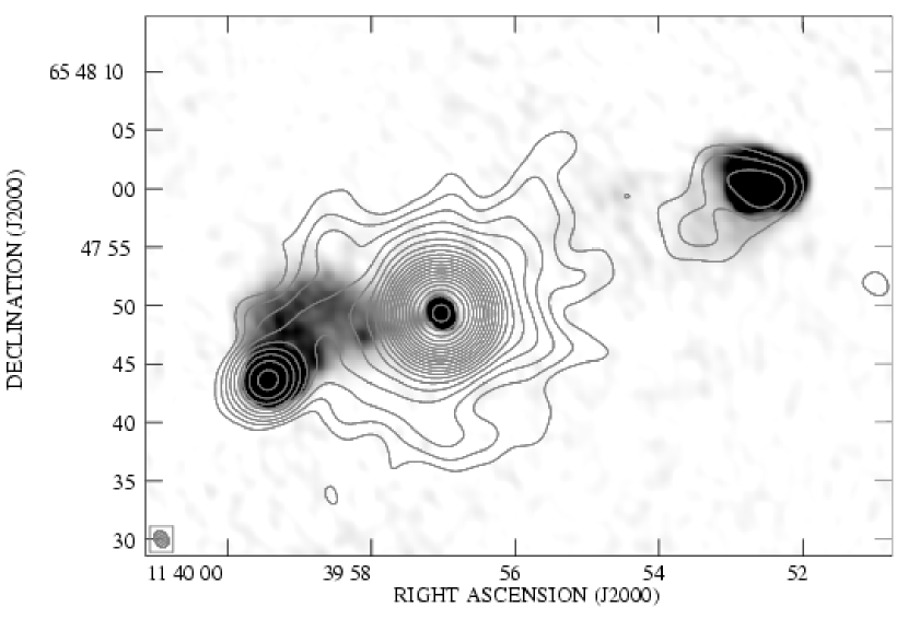
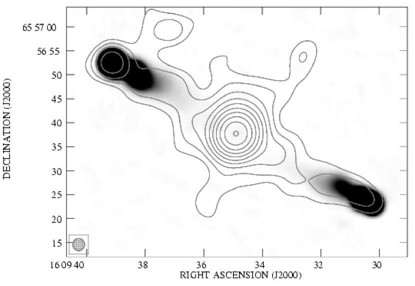
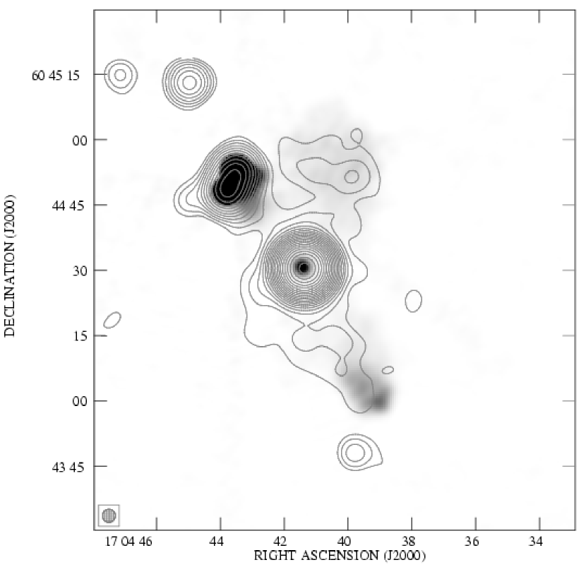
Figure 1: The three X-ray sources. From top to bottom: 3C 263, 3C 330 and 3C 351. The contours show the X-ray data, smoothed with a Gaussian of FWHM $3\farcs 5$ (for 3C 263) and $6\arcsec$ (for the other two sources): the contour intervals are logarithmic in steps of $\sqrt{2}$ and the lowest contour in each figure is the $3\sigma$ level as defined by Hardcastle (2001). The objects to the NE and S of 3C 351 are background point sources. The greyscales show radio maps. The map of 3C 263 is a 1.4-GHz VLA image with $1\farcs 5\times 1\farcs 1$ resolution; black is 10 mJy beam^-1. The 3C 330 and 3C 351 maps are 8.4-GHz VLA images, from Gilbert et al. (2002), with 3″ resolution; black is 10 mJy beam^-1.

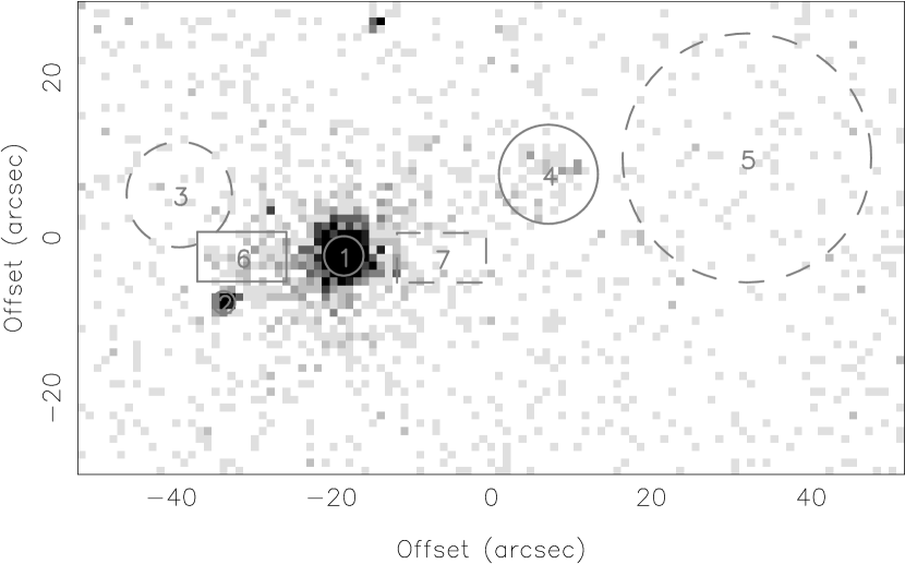
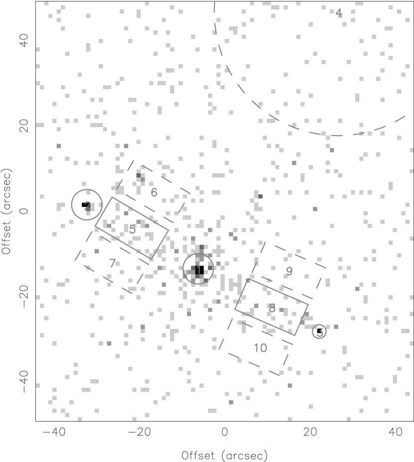
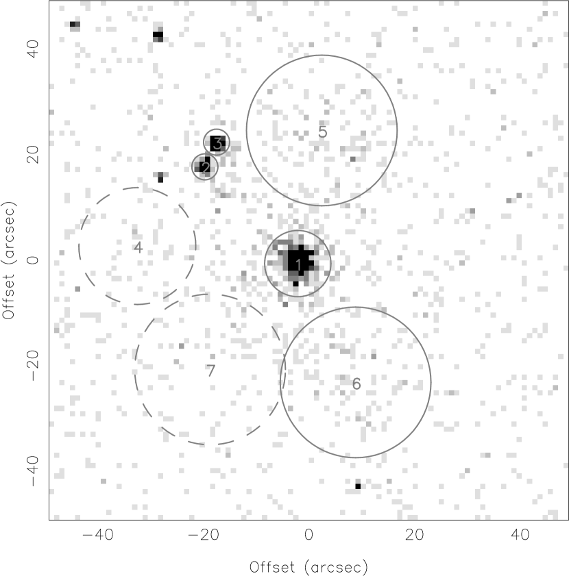
Figure 2: Extraction regions used in the three radio sources. From top to bottom: 3C 263, 3C 330 and 3C 351. Each image shows the 0.4-7 keV events binned by a factor of 2 (i.e. to 0$\farcs$984 pixels); black is 8, 5 and 8 counts per bin respectively. Solid lines show source regions, and dashed lines background regions. Numbers refer to the regions listed in Table 7. For clarity, a few regions have been omitted.

Table 7: Spatial regions used in extraction

Source	Component	Central position	Geometry	Number
3C 263	Core	$11^{\rm h}39^{\rm m}57\fs 025$, $+65\arcdeg 47^{\prime}49\farcs 36$	Circle, $r=5$ pixels	1
	SE hotspot (IJK)	$11^{\rm h}39^{\rm m}59\fs 457$, $+65\arcdeg 47^{\prime}43\farcs 59$	Circle, $r=2.9$ pixels	2
	SE hotspot (K)	$11^{\rm h}39^{\rm m}59\fs 492$, $+65\arcdeg 47^{\prime}43\farcs 47$	Circle, $r=1.4$ pixels
	SE hotspot background	$11^{\rm h}40^{\rm m}00\fs 361$, $+65\arcdeg 47^{\prime}57\farcs 06$	Circle, $r=13.4$ pixels	3
	NW hotspot (limit region)	$11^{\rm h}39^{\rm m}52\fs 857$, $+65\arcdeg 47^{\prime}59\farcs 57$	Circle, $r=12.6$ pixels	4
	NW lobe	$11^{\rm h}39^{\rm m}52\fs 857$, $+65\arcdeg 47^{\prime}59\farcs 57$	Circle, $r=12.6$ pixels	4
	NW lobe background	$11^{\rm h}39^{\rm m}48\fs 821$, $+65\arcdeg 48^{\prime}01\farcs 59$	Circle, $r=31.6$ pixels	5
	Jet (limit region)	$11^{\rm h}39^{\rm m}59\fs 090$, $+65\arcdeg 47^{\prime}49\farcs 30$	Box, $22.6\times 12.6$ pixels, $90\arcdeg$	6
	SE lobe	$11^{\rm h}39^{\rm m}59\fs 090$, $+65\arcdeg 47^{\prime}49\farcs 30$	Box, $22.6\times 12.6$ pixels, $90\arcdeg$	6
	SE lobe background	$11^{\rm h}39^{\rm m}55\fs 030$, $+65\arcdeg 47^{\prime}49\farcs 16$	Box, $22.6\times 12.6$ pixels, $90\arcdeg$	7
3C 330	Core	$16^{\rm h}09^{\rm m}34\fs 896+65\arcdeg 56^{\prime}37\farcs 69$	Circle, $r=7.3$ pixels	1
	NE hotspot	$16^{\rm h}09^{\rm m}39\fs 155$, $+65\arcdeg 56^{\prime}52.79$	Circle, $r=7.3$ pixels	2
	SW hotspot	$16^{\rm h}09^{\rm m}30\fs 255$, $+65\arcdeg 56^{\prime}23.07$	Circle, $r=3.25$ pixels	3
	Hotspot/core background	$16^{\rm h}09^{\rm m}41\fs 548$, $+65\arcdeg 56^{\prime}13.74$	Circle, $r=65.5$ pixels	4
	NE lobe	$16^{\rm h}09^{\rm m}37\fs 433$, $+65\arcdeg 56^{\prime}47.29$	Box, $31.1\times 16.0$ pixels, $59.5\arcdeg$	5
	NE lobe background	$16^{\rm h}09^{\rm m}36\fs 608$, $+65\arcdeg 56^{\prime}55.90$	Box, $31.1\times 16.0$ pixels, $59.5\arcdeg$	6
		$16^{\rm h}09^{\rm m}38\fs 198$, $+65\arcdeg 56^{\prime}39.30$	Box, $31.1\times 16.0$ pixels, $59.5\arcdeg$	7
	SW lobe	$16^{\rm h}09^{\rm m}32\fs 083$, $+65\arcdeg 56^{\prime}28.83$	Box, $31.1\times 16.0$ pixels, $66.5\arcdeg$	8
	SW lobe background	$16^{\rm h}09^{\rm m}31\fs 419$, $+65\arcdeg 56^{\prime}37.44$	Box, $31.1\times 16.0$ pixels, $66.5\arcdeg$	9
		$16^{\rm h}09^{\rm m}32\fs 687$, $+65\arcdeg 56^{\prime}19.49$	Box, $31.1\times 16.0$ pixels, $66.5\arcdeg$	10
3C 351	Core	$17^{\rm h}04^{\rm m}41\fs 364$, $+60\arcdeg 44^{\prime}30\farcs 46$	Circle, $r=12.8$ pixels	1
	Core background	$17^{\rm h}04^{\rm m}41\fs 364$, $+60\arcdeg 44^{\prime}30\farcs 46$	Annulus, $r=12.8..25$ pixels
	N hotspot (J)	$17^{\rm h}04^{\rm m}43\fs 781$, $+60\arcdeg 44^{\prime}48\farcs 20$	Circle, $r=5$ pixels	2
	N hotspot (L)	$17^{\rm h}04^{\rm m}43\fs 479$, $+60\arcdeg 44^{\prime}52\farcs 88$	Circle, $r=5$ pixels	3
	N hotspots background	$17^{\rm h}04^{\rm m}45\fs 525$, $+60\arcdeg 44^{\prime}33\farcs 19$	Circle, $r=22.5$ pixels	4
	S hotspot (limit region)	$17^{\rm h}04^{\rm m}39\fs 754$, $+60\arcdeg 44^{\prime}04\farcs 91$	Circle, $r=16$ pixels
	N lobe	$17^{\rm h}04^{\rm m}40\fs 760$, $+60\arcdeg 44^{\prime}55\farcs 09$	Circle, $r=29$ pixels	5
	S lobe	$17^{\rm h}04^{\rm m}39\fs 888$, $+60\arcdeg 44^{\prime}07\farcs 37$	Circle, $r=29$ pixels	6
	Lobe background	$17^{\rm h}04^{\rm m}43\fs 646$, $+60\arcdeg 44^{\prime}09\farcs 83$	Circle, $r=29$ pixels	7

Note. — Positions quoted are corrected to the frame defined by the radio observations, as discussed in the text. One Chandra pixel is $0\farcs 492$. ‘Limit regions’ are the regions used to determine a background count rate for an upper limit on a compact component; smaller detection regions are then used to derive the upper limit, as discussed in the text. Box regions are given as long axis $\times$ short axis, position angle of long axis (defined north through east). Numbers refer to the regions shown in Fig. 2.

Table 8: X-ray properties of source components

Source	Component	Net count rate	Net counts	Spectral fit	$\chi^{2}/n$	2–10 keV flux	1-keV flux
		(0.4–7.0 keV,				($\times 10^{-15}$ ergs	density (nJy)
		s-1)				cm-2 s-1)
3C 263	Core	$0.163\pm 0.002$	$7218\pm 85$	$\alpha=0.75\pm 0.06$	229/199	$1700\pm 300$	$290\pm 30$
	SE hotspot (IJK)	$(2.5\pm 0.5)\times 10^{-3}$	$110\pm 22$	$\alpha=1.2\pm 0.2$	1.4/3	$5.1\pm 0.5$	$1.7\pm 0.2$
	SE hotspot (K)	$(1.6\pm 0.2)\times 10^{-3}$	$69\pm 8$	$\alpha=1.0\pm 0.3$	0.64/1	$3.6\pm 0.4$	$1.0\pm 0.1$
	NW hotspot (B)	$<1\times 10^{-4}$	$<4$	…	…	…	$\lesssim 0.06$
	Jet	$<5\times 10^{-4}$	$<20$	…	…	…	$\lesssim 0.3$
	NW lobe	$(1.2\pm 0.2)\times 10^{-3}$	$53\pm 7$	$\alpha=0.4\pm 0.2$	0.98/1	$7.8\pm 1.8$	$0.8\pm 0.2$
	SE lobe	$(7.7\pm 2.2)\times 10^{-4}$	$34\pm 10$	…	…	…	$0.5\pm 0.2$
3C 330	Core	$(3.4\pm 0.5)\times 10^{-3}$	$150\pm 22$	$\alpha_{1}=0.8_{-0.4}^{+0.5}+[N_{\rm H}=(4\pm 2)\times 10^{23}$ cm-2, $\alpha_{2}=1.6^{+2.7}_{-1.3}]$	1.8/2	$47\pm 7$	$1.5\pm 0.2$
	NE hotspot	$(5.0\pm 1.1)\times 10^{-4}$	$22\pm 5$	…	…	…	$0.34\pm 0.07$
	SW hotspot	$(1.3\pm 0.6)\times 10^{-4}$	$6\pm 3$	…	…	…	$0.09\pm 0.04$
	NE lobe	$(4.1\pm 1.5)\times 10^{-4}$	$18\pm 7$	…	…	…	$0.28\pm 0.10$
	SW lobe	$(4.7\pm 1.2)\times 10^{-4}$	$21\pm 5$	…	…	…	$0.32\pm 0.08$
3C 351	Core	$0.160\pm 0.002$	$7310\pm 91$	$\alpha_{1}=2.5\pm 0.3+[N_{\rm H}=(1.1\pm 0.1)\times 10^{22}$ cm-2, $\alpha_{2}=0.46\pm 0.05]$	304/212	$1560\pm 20$	$14\pm 3$
	N hotspot (J)	$(6.5\pm 0.5)\times 10^{-3}$	$297\pm 23$	$\alpha=0.5\pm 0.1$	8/11	$36\pm 4$	$4.3\pm 0.3$
	N hotspot (L)	$(5.2\pm 0.5)\times 10^{-3}$	$238\pm 23$	$\alpha=0.85\pm 0.1$	17/9	$17\pm 2$	$3.4\pm 0.4$
	S hotspot	$<0.7\times 10^{-4}$	$<3$	…	…	…	$\lesssim 0.05$
	N lobe	$(1.3\pm 0.3)\times 10^{-3}$	$59\pm 14$	$\alpha=0.6\pm 0.8$	0.6/1	$8\pm 2$	$1.1\pm 0.3$
	S lobe	$(0.9\pm 0.3)\times 10^{-3}$	$41\pm 14$	$\alpha=0.6\pm 0.8$	0.6/1	$5\pm 2$	$0.7\pm 0.3$

Note. — 2-10 keV fluxes quoted are absorbed, observer-frame values. The observer-frame 1-keV flux densities tabulated are corrected for Galactic absorption, which is fixed to the previously measured value (Table 2) in all fits. Errors quoted are $1\sigma$ for one interesting parameter.

3.2 Intra-cluster medium emission

Our deep Chandra observations also allow us to search for extended, cluster-related X-ray emission. Extended emission, on scales larger than the radio lobes, was visible by eye in the observations of 3C 263 and 3C 330. To characterize this extended emission we masked out the readout streak and the non-nuclear emission (hotspots and lobes), using conservatively large masking regions which effectively covered the whole extended radio source in each case, and then generated a radial profile for each object. We chose to represent the extended emission with isothermal $\beta$ models (Cavaliere & Fusco-Femiano, 1978), which give rise to an angular distribution of counts on the sky of the form

$$b_{\rm X}(\theta)=b_{0}\left(1+{\theta^{2}\over\theta_{c}^{2}}\right)^{{1\over 2}-3\beta}$$

where $b_{\rm X}$ is the count density (in count arcsec^-2) as a function of off-source angle $\theta$, $b_{0}$ is the central count density, and $\theta_{c}$ and $\beta$ parametrize the angular scale and shape of the extended emission. Modelling the background-subtracted radial profiles as a combination of a delta function and a $\beta$ model, both convolved with the point spread function (PSF), we then carried out least-squares fits using a grid of $\beta$ and $\theta_{c}$ values to find out whether extended emission was required and to determine the best-fitting $\beta$ model parameters.

To do this we required an analytical model of the PSF. Worrall et al. (2001a, 2001b) discussed the fitting of analytical forms to data from the ciao PSF library, and our approach is similar. Our data are derived from the ciao mkpsf command, energy-weighted to reflect the approximate energy distribution of the observed data in the extraction radius, smoothed with a small Gaussian to simulate the effects of pixelation and aspect uncertainties, and then fitted with a suitable function of radius. The forms used by Worrall et al., though a good fit to the inner regions of the PSF and so adequate for the purposes used in their papers, do not represent the wings found at radial distances of tens of arcsec, and these are important in the case of 3C 263 and 3C 351, where the emission is dominated by the bright central point source out to large radii. Accordingly, we fit a functional form consisting of two Gaussians, two exponentials and a power-law component, which we found empirically to be a good fit out to large distances, to the PSF $a(\theta)$:

$$a(\theta)=a_{1}\exp\left(-{{\theta^{2}}\over 2s_{1}^{2}}\right)+a_{2}\exp\left(-{{\theta^{2}}\over 2s_{2}^{2}}\right)+a_{3}\exp\left(-{\theta\over s_{3}}\right)+a_{4}\exp\left(-{\theta\over s_{4}}\right)+a_{5}\left(1+{\theta\over\theta_{n}}\right)^{s_{5}}$$

where $a_{1}..a_{5}$, $s_{1}..s_{5}$ are parameters of the fit and $\theta_{n}$ is a fixed normalizing value. In practice, the power-law index $s_{5}$ was determined using the lowest-resolution PSF libraries, and then fixed while the other parameters were determined from higher-resolution data. In using a power-law model for the PSF wings, we have followed other work on characterizing the large-radius PSF (see, e.g., documents at URL: $<$http://asc.harvard.edu/cal/Hrma/hrma/psf/$>$) and we have obtained similar power-law indices, $s_{5}\approx 2.0$, in all the fits we have carried out.

3.3 Inverse-Compton modeling

To compare the observed X-ray emission from the lobes and hotspots to the predictions of inverse-Compton models it is necessary to know the spatial and spectral structure of these components in the radio and optical in as much detail as possible. The available data in these bands are discussed in the following sections, but in each case we extracted and tabulated radio flux densities (Table 9) and derived radio-based models for the hotspots and lobes. Where these components were well resolved, we measured their sizes directly from radio maps; where they were compact, as was the case for some of the hotspots, we characterized the component size by fitting a model of the emission from an optically thin homogeneous sphere, convolved with the restoring Gaussian, to the high-resolution radio maps.

We then used a computer code to predict inverse-Compton flux density as a function of magnetic field strength. Two inverse-Compton codes were available to us. One, described by Hardcastle et al. (1998), treats all inverse-Compton sources as homogeneous spheres; this allows us to neglect the anisotropy of inverse-Compton emission, and so gives a quick and simple calculation. Our other code is based on the results of Brunetti (2000). By incorporating Brunetti’s formulation of anisotropic inverse-Compton scattering, this code allows us to take account of the spatial and spectral structure of the resolved hotspots. To model spatial structure, the hotspots are placed on a fine three-dimensional grid and the emissivity resulting from the illumination of every cell by every other cell is calculated (making small corrections for self-illumination and nearest-neighbour effects). To do this in full generality is computationally expensive, since it requires numerical integration of equations A1–5 of Brunetti (2000) over the electron distribution and incoming photon distribution for each cell in an $O(n^{6})$ algorithm, where $n$ is the number of cells in one dimension of the three-dimensional grid. We solve this problem by allowing only a small number of distinct electron spectra and magnetic fields in our grid. This means that the task of calculating the illumination of a region of electrons of a given spectral shape by a given photon distribution reduces to one of tabulating the integral of Brunetti’s results for a suitably sampled subset of the possible values of the geometry parameter $k_{3}$. Since the dependence on the normalization of the electron energy spectrum and on the incoming photon flux is linear, the $O(n^{6})$ part of the algorithm then just involves an interpolation and multiplication. For homogeneous spheres, or in the case of cosmic microwave background (CMB) inverse-Compton scattering (CMB/IC) where anisotropy is not an issue, the results of our two codes agree to within a few per cent, and so in the results presented below we use whichever code is most appropriate for a particular situation.

The synchrotron spectra of the hotspots and lobes studied in this work are not as well studied as those of earlier targets, so some assumptions are necessary in modeling them. Our basic model is a broken power-law electron energy spectrum, such that

$$N(\gamma)=\cases{0&$\gamma<\gamma_{\rm min}$\cr N_{0}\gamma^{-p}&$\gamma_{\rm min}<\gamma<\gamma_{\rm break}$\cr N_{0}(\gamma_{\rm break}^{d})\gamma^{-(p+d)}&$\gamma_{\rm break}<\gamma<\gamma_{\rm max}$\cr 0&$\gamma>\gamma_{\rm max}$\cr}$$

where $N(\gamma){\rm d}\gamma$ gives the number density of electrons with Lorentz factors between $\gamma$ and $\gamma+{\rm d}\gamma$. We choose this model because synchrotron theory tells us that it is a good approximation to the expected situation in hotspots, where particle acceleration and synchrotron losses are competing; for $d=1$ it approximates the standard ‘continuous injection’ model, which applies to a region containing the acceleration site and a downstream region of synchrotron radiation loss (e.g., Heavens & Meisenheimer, 1987). Theoretical prejudice (based on models of shock acceleration) also suggests a value $p=2$ for the low-energy power-law index (the ‘injection index’). This electron energy spectrum gives rise to a synchrotron spectrum whose spectral index $\alpha$ is flat or inverted ($\alpha=-1/3$) around and below some frequency $\nu_{\rm turn}$, has a value 0.5 up to around some break frequency $\nu_{\rm break}$ and then steepens to a value of 1.0 before an exponential cutoff around some frequency $\nu_{\rm cutoff}$. Such models have been successfully fit to a number of well-studied hotspots (e.g., Meisenheimer et al., 1989; Looney & Hardcastle, 2000). It is well known that the synchrotron turnover, break and cutoff are not sharp; for typical parameters of a radio source they occupy a decade or more in frequency. It is for this reason that we prefer to work with the well-defined and physically interesting quantities $\gamma_{\rm min}$, $\gamma_{\rm break}$, $\gamma_{\rm max}$, whose only disadvantage is that they must be specified together with a value of the magnetic field strength $B$. We typically work with the equipartition magnetic field strength, $B_{\rm eq}$, which is given by

$$m_{\rm e}c^{2}\int_{\gamma_{\rm min}}^{\gamma_{\rm max}}\gamma N(\gamma){\rm d}\gamma=B_{\rm eq}^{2}/2\mu_{0}$$

(where we have assumed that equipartition is between the radiating electrons and the magnetic field only, and where SI units are used, with $\mu_{0}$ being the permeability of free space).

$\gamma_{\rm max}$ is constrained if there is evidence for spectral steepening to $\alpha>1$ in the synchrotron spectrum. We find that $\gamma_{\rm break}$ is often in the observed radio region, so that it is relatively easy to constrain. We therefore estimate $\gamma_{\rm max}$ and $\gamma_{\rm break}$ using least-squares fitting to the radio and optical data. (Typically $\gamma_{\rm max}$ lies above the radio region, in which case its value has little effect on our inverse-Compton calculations.) $\gamma_{\rm min}$, however, can only be directly constrained by observations of a low-frequency turnover in sources which are not synchrotron self-absorbed (Carilli et al., 1991; Hardcastle et al., 2001a; Hardcastle, 2001) or by observations of optical inverse-Compton emission (Hardcastle, 2001) and neither of these methods has yet been applied to the hotspots or lobes of our sources. Our low-frequency data on the hotspots typically constrain $\gamma_{\rm min}\lesssim 1000$ for equipartition fields, but values of $\gamma_{\rm min}$ between 400 and 1000 have been reported for other objects (Hardcastle, 2001, and references therein). In addition, it is possible, as argued by Brunetti et al. (2002a), that the electron spectrum at low energies should be modified by the effects of adiabatic expansion out of the hotspot. Fortunately, the values of $\gamma_{\rm min}$ and the low-energy electron spectral shape have only a small effect on the inverse-Compton calculation, because the broken synchrotron spectrum produces few high-energy photons that can be scattered into the X-ray by such low-energy electrons. Unless otherwise stated we assume $\gamma_{\rm min}=1000$.

Table 9: Radio flux densities for source components

Source	Component	Model	Frequency	Flux density
			(GHz)	(mJy)
3C 263	Hotspot K	Sphere, $r=0\farcs 39$	1.4	1670
			4.8	591
			8.3	303
			14.9	184
			84.9	54
	Hotspot B	Sphere, $r=0\farcs 18$	4.8	23
			8.3	16
			14.9	9
	S lobe (X-ray region)	Cube, $9\farcs 5\times 6\farcs 3\times 9\farcs 3$	1.4	206
			4.9	45
	N lobe	Sphere, $r=6\arcsec$	1.4	550
			4.9	188
3C 330	NE hotspot	Cylinder, $2\farcs 3\times 0\farcs 64$	1.5	3830
			8.4	755
			14.9	376
			84.9	25
	SW hotspot	Sphere, $r=0\farcs 19$	8.4	0.77
	NE lobe (X-ray region)	Cylinder, $15\arcsec\times 2\farcs$6	1.5	737
			8.4	161
			14.9	63
	SW lobe (X-ray region)	Cylinder, $15\arcsec\times 2\farcs 6$	1.5	768
			8.4	135
			14.9	55
3C 351	Hotspot J	Sphere, $r=0\farcs 16$	1.4	530
			8.4	130
			15.0	88
			84.9	17
	Hotspot L	Sphere, $r=0\farcs 8$	1.4	1300
			8.4	316
			15.0	201
			84.9	28
	Hotspot A	Two spheres, $r=0\farcs 35$	8.4	3
	N lobe (X-ray region)	Sphere, $r=10.5\arcsec$	1.4	283
			8.3	43
	S lobe (X-ray region)	Cylinder, $28\arcsec\times 6\farcs 5$	1.4	248
			8.3	46

Note. — Errors on the hotspot flux densities are due primarily to flux calibration uncertainties, nominally 2% for the VLA data and 10% for the 85-GHz BIMA data, as discussed in §2.

4 3C 263

4.1 Introduction

3C 263 is a $z=0.66$ quasar. In the radio, the best maps are those of Bridle et al. (1994, hereafter B94), who show it to have a one-sided jet which points towards a bright, compact hotspot in the SE lobe. The source lies in an optically rich region, and some nearby objects’ associations with the quasar have been spectroscopically confirmed; HST observations show several close small companions. Deep X-ray images were made with ROSAT by Hall et al. (1995) in an attempt to locate the X-ray emission from the host cluster, but no significant extended emission on cluster scales was found by them or by Hardcastle & Worrall (1999) who re-analysed their data. The ROSAT data were dominated by the quasar’s bright, variable nuclear X-ray component.

4.2 Core

The bright X-ray nucleus of 3C 263 suffers from pileup in our full-frame observation. The piled-up count rate over the full Chandra band is $0.190\pm 0.002$ s^-1, so that we would expect a pileup fraction of about 20%. When the core is fitted with a power-law spectrum without making any correction for pileup, there is no sign of any excess absorption over the (small) Galactic value, but the best-fit power-law is very flat ($\alpha\approx 0.1$) and there are substantial residuals around 2 keV, which are both characteristic of piled-up spectra. Using the pileup model in xspec, which implements the work of Davis (2001), we find a good fit with a range of steeper power-laws. Following Davis (2001) we fix the grade correction parameter $\bar{g}_{0}$ to 1 and allow only the grade morphing parameter to vary. We find the best fit (Table 8) to have $\alpha=0.75\pm 0.06$ (since the slope and normalization are strongly correlated in this model, the error quoted is $1\sigma$ for two interesting parameters), which is in reasonable agreement with previous observations; for example, in the compilation of Malaguti et al. (1994) $\alpha$ values between 0.7 and 1.0 are reported. The pileup-corrected 1-keV flux density is substantially lower than the value we estimated (based on a similar spectral assumption) from the ROSAT HRI data (Hardcastle & Worrall, 1999), suggesting variability by a factor of $\sim 2$ on a timescale of years (the ROSAT data were taken in 1993). This is consistent with the observations of Hall et al. (1995), who saw variability by a factor 1.5 in 18 months.

Using the default Chandra astrometry, the core centroid is at $11^{\rm h}39^{\rm m}57\fs 170$, $+65\arcdeg 47^{\prime}49\farcs 22$, while our best position for the radio core, using our 15-GHz VLA data, is $11^{\rm h}39^{\rm m}57\fs 025$, $+65\arcdeg 47^{\prime}49\farcs 36$, which is within $0\farcs 05$ of the position quoted by B94. The Chandra position is thus offset by approximately $0\farcs 89$ in RA and $0\farcs 14$ in declination from the radio data, which is consistent with known Chandra astrometric uncertainties. In our spatial analysis we shift the Chandra data so that the core positions match, and align other radio and HST data with our best core position.

4.3 Hotspots

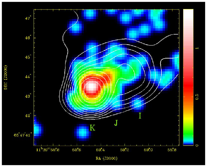
Figure 3: The radio and X-ray hotspot of 3C 263. The X-ray hotspot is smoothed with a $0\farcs 5$ Gaussian. Overlaid are 5-GHz radio contours at a resolution of $0\farcs 85$, approximately matched to the Chandra data. These are logarithmic in steps of 2, starting at 0.5 mJy beam^-1. The labels K, H and I refer to features of the radio emission discussed in the text, following the notation of B94.

The bright SE hotspot of 3C 263 is detected in the Chandra observation; it corresponds to a faint feature seen in the ROSAT HRI images by Hall et al. (1995), which they describe as a ‘clump’ of X-ray emission. As Fig. 3 shows, we detect emission with Chandra not just from the compact component K (we use the notation of B94) but also the faint tail J (which may trace the incoming jet) and the trailing plateau of emission I. The X-ray/radio ratio is considerably higher in J (by a factor $\sim 4$) than in the other components. The high-resolution images show that the X-ray centroid of the compact component K is slightly to the north of the peak of the radio emission. The offset is about $0\farcs 3$, or 2 kpc. The angular displacement about the pointing centre, 1.1°, is too large by an order of magnitude to be due to Chandra roll uncertainties, which are typically at most 0.1° (Aldcroft, private communication); we conclude that the offset is real. We extracted spectra from the entire complex IJK and from the compact hotspot K. The net count rate from the IJK complex is consistent, within the errors, with the count rate estimated by Hall et al. for the ‘clump’ in their ROSAT data, converted to an equivalent Chandra count rate.

A faint optical counterpart to K is detected in the 1000-s F675W HST observation of 3C 263 (Fig. 4). After aligning the radio core with the peak of the optical quasar emission, the peak optical and radio positions of the hotspot agree to within $0\farcs 1$. (HST roll uncertainties are usually no worse than $0.05\arcdeg$, corresponding to an error at this distance from the pointing centre of $0\farcs 01$.) We estimate a flux density for this component at $4.5\times 10^{14}$ Hz of $0.8\pm 0.4$ $\mu$Jy, with the large error arising because of uncertainties in background estimation.

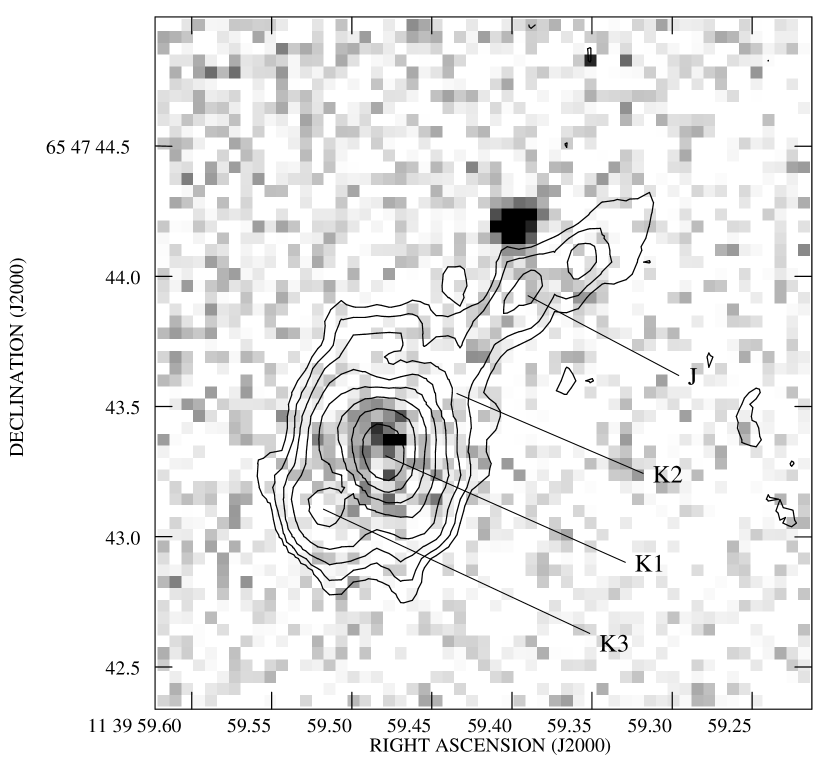
Figure 4: Optical hotspot of 3C 263 with high-resolution radio data. The greyscale runs between 4 and 11 HST counts per PC pixel. The radio map is the 15-GHz map at full resolution ($0\farcs 14\times 0\farcs 10$). The lowest radio contour is at 0.2 mJy beam^-1 and the contours increase logarithmically by a factor 2. The components K1, K2, K3 of hotspot K, and the linear feature J, discussed in the text, are labeled.

Figure 5: The source-frame spectrum of hotspot K of 3C 263. Radio points from Table 9, the optical HST flux density and the X-ray flux density are plotted together with the two-component synchrotron model with $\gamma_{\rm min}=1000$ discussed in the text (dashed lines show the two components, solid line shows the total) and the predicted total SSC emission (dot-dashed line) and CMB/IC emission (dotted line) in this model at equipartition.

As Fig. 4 shows, the hotspot has considerable spatial structure in the radio. Even the compact component K is shown by our 15-GHz images to have several sub-components; a bright central component K1, an extended halo K2, and a weak leading compact component K3. The radio spectrum of hotspot K (Fig. 5), which we obtain by Gaussian fitting to the 1.4-GHz map and by integration of matched regions on the higher-resolution 4.8, 8.3 and 15-GHz maps, also shows signs of multiple structure, in that the spectrum steepens between 4.8 and 8.3 GHz but then flattens again between 8.3 and 15 GHz. 8.4–15 GHz spectral index maps show that the compact central component K1 has a flatter two-point radio spectrum, $\alpha\approx 0.8$, while the surrounding material is steeper-spectrum, $\alpha\approx 1.0$. Correcting for background contamination, $\alpha_{\rm K1}\approx 0.7$ between 8.3 and 15 GHz, which is consistent with the observed 15-85 GHz spectral index. We can crudely model hotspot K as being a superposition of two of our standard spectra with different break frequencies, with the K1 component breaking above 85 GHz ($\gamma_{\rm break}\approx 2\times 10^{4}$, assuming equipartition magnetic fields) while the K2/3 components break at 1.4 GHz or lower ($\gamma_{\rm break}\approx 1000$). In order for the K1 component not to overproduce the observed optical emission, assumed to be synchrotron emission, its spectrum must then steepen further at high energies; we choose to model this with a high-energy cutoff in the electron energy spectrum, $\gamma_{\rm max}=5\times 10^{5}$. For simplicity, we assign the extended component the same high-energy cutoff, which makes its contribution to the observed optical emission negligible. We modeled K1 as a sphere of radius $0\farcs 15$ and K2 as a sphere of radius $0\farcs 39$, based on the 15-GHz map. This synchrotron model is plotted in Fig. 5).

Three important unknown factors remain: the geometry of K1/K2 (does the compact component K1 lie inside or outside, in front of or behind, the more extended component K2?), the spatial electron distribution in the two spheres (uniform or centrally peaked? the radio data are not good enough to say) and the low-energy cutoff in the synchrotron spectrum. The 1.4-GHz observations suggest a low-energy cutoff $\gamma_{\rm min}\lesssim 1000$; a higher cutoff would mean we would start to observe spectral flattening at this frequency. We carried out our inverse-Compton modeling with a range of possible geometries, spatial electron distributions and $\gamma_{\rm min}$ values in order to assess the effect of these differences. We find that the most significant effect is given by a more centrally peaked distribution of electrons; $\gamma_{\rm min}$ has little effect, and only if K1 and K2 are widely separated is a significant difference made by the geometry (arising because of the weaker mutual illumination of K1 and K2). The overall conclusion from this modeling is that for equipartition magnetic fields (where equipartition in this case means that equipartition holds separately for each spectral component) the inverse-Compton flux density from hotspot K is typically less than the observed value by a factor $\sim 3.5$. To produce the observed X-ray flux density by the inverse-Compton process, the magnetic field strengths in the two components of the hotspot must be lower than the equipartition value by a factor 1.9 (for the case where the compact component is at the center of the extended component), so that the compact component has $B=15$ nT and the extended component has $B=7$ nT. The predicted X-ray spectral index at an observed energy of 1 keV is then 0.75, which is consistent within the $1\sigma$ error with the observed value, $1.0\pm 0.3$. This conclusion is robust to changes in the model parameters; for example, even a simple homogeneous spherical model, while giving different values for the equipartition magnetic field strength, predicts a net inverse-Compton flux density of 0.26 nJy and requires a factor $\sim 2$ decrease in field to reproduce the observed X-rays.

The comparatively strong detection of component J is puzzling. Its 1-keV flux density is $\sim 0.35\pm 0.1$ nJy, assuming spectral parameters similar to those of K. If the X-ray emission corresponds to the narrow feature seen in Fig. 4, it is much too bright to be SSC at or close to equipartition. A long, thin cylinder is a very poor SSC source, and the equipartition 1-keV flux density of this component should be $\sim 2$ pJy, including scattering of photons from K1 and K2. The magnetic field would have to be lower than equipartition by a factor $\sim 20$ if all the X-ray flux were to be produced by component J by the SSC and invese-Compton processes. If there is significant relativistic motion in J, then in its frame the emission from K and from the CMB is enhanced, and this can increase the net X-ray emissivity; however, it is hard to achieve the required increase without very large bulk Lorentz factors and small angles to the line of sight. Our model here is unrealistically simple, as it does not take acount of the extended emission around J: however, it seems clear that this region is significantly different from hotspot K.

The much fainter NW compact hotspot, B in the notation of B94, is not detected in X-rays. Assuming that the source is unresolved to Chandra and using a detection cell of 6 standard Chandra pixels (the 80% encircled energy criterion, as used by celldetect), we can place a $3\sigma$ upper limit on its count rate of $1\times 10^{-4}$ s^-1 over the 0.4-7.0 keV energy band, estimating the background count level from the region around the hotspot, and convert this to a limit on flux density by using the spectrum of the detected hotspot. No optical counterpart to this hotspot is visible in the HST image. Its predicted inverse-Compton X-ray flux density, assuming similar electron spectral parameters to those used for hotspot K, a homogenous spherical model, and an equipartition magnetic field, is 5 pJy, an order of magnitude below our upper limit. We can say only that $B$ cannot be more than a factor $\sim 4$ below $B_{\rm eq}$ in this hotspot.

4.4 Jet

There is no evidence of X-ray emission from 3C 263’s jet in the data, with the possible exception of the hotspot-related feature J, discussed above. The jet is $11\farcs 6$ long in the radio images of B94 and is essentially unresolved transversely at their highest resolution of $0\farcs 35$. Using a background region in the SE lobe, we estimate a $3\sigma$ upper limit on its count rate, as tabulated in Table 8. We convert this to an upper limit on the jet X-ray flux density by using the spectrum of the detected hotspot.

The radio flux density of the jet is only 8 mJy at 5 GHz, so that its radio to X-ray spectral index is $\gtrsim 1.0$. If the X-ray emission from quasar jets is boosted inverse-Compton scattering from the CMB, as suggested by various authors (e.g., Tavecchio et al., 2000), then its expected X-ray flux density depends on the bulk Lorentz factor $\Gamma$ and the angle made by the jet to the line of sight $\theta$. We find the upper limit to be inconsistent only with extreme models of the jet, with $\Gamma\gtrsim 7$ and $\theta\lesssim 10\arcdeg$. The overall appearance of the source suggests that the angle to the line of sight is a good deal larger than this, in which case even larger bulk Lorentz factors are not ruled out by the X-ray data.

4.5 Lobes

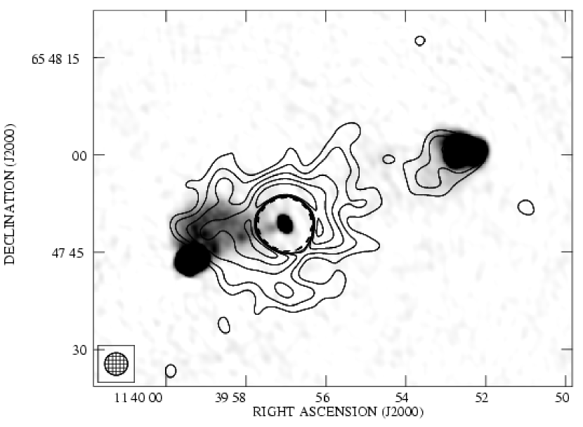
Figure 6: The lobes and extended emission of 3C 263. The contours show the X-ray emission smoothed with a $3\farcs 5$ (FWHM) Gaussian. The hotspot regions were masked out before smoothing and a scaled, smoothed, energy-weighted PSF model was subtracted from the image after smoothing to remove the nuclear emission. Because the X-ray core of 3C 263 is piled up, this subtraction leaves some residuals at the center of the smoothed image. The lowest contour is the $3\sigma$ level, defined according to the prescription of Hardcastle (2000), and the contours increase logarithmically by a factor $\sqrt{2}$. The FWHM of the convolving Gaussian is shown in the bottom left-hand corner. The greyscale shows a 1.4-GHz VLA image with $1\farcs 5\times 1\farcs 1$ resolution; black is 10 mJy beam^-1.

X-ray emission is detected from the lobes of 3C 263 (Fig. 6). Although the detection of the NW lobe emission is more obvious, because it is further from the core and there is no compact hotspot emission, we also detect excess counts from the SE lobe.

For inverse-Compton calculations we model both lobes with similar broken power-law electron distributions. We take $\gamma_{\rm min}$ here to be 100 rather than 1000, to take some account of the effects of adiabatic expansion; the inverse-Compton prediction is insensitive to this choice. $\gamma_{\rm break}$ is required to correspond to a frequency near the radio region, to produce the steep spectrum of the lobes, and we model both lobes with high-energy cutoffs in the radio region, $\gamma_{\rm max}\sim 2\times 10^{4}$. The predicted 1-keV CMB/IC flux densities on this model (which treats the lobes as uniform) are 0.13 nJy for the S lobe and 0.2 nJy for the N lobe, a factor $\sim 4$ below the observed flux densities in both cases. The magnetic field strength in the lobes must be a factor $\sim 2$ below the equipartition value if the lobe X-ray emission is to be produced by inverse-Compton scattering of the CMB. With this reduction in field strength, the pressures in the lobes due to electrons and magnetic field are between 1.5 and $2.0\times 10^{-12}$ Pa.

4.6 Extended emission

Figure 7: Background-subtracted radial profile of 3C 263 after hotspot- and lobe-related emission has been masked out. The two light solid lines show the PSF (steeper slope) and extended model (flatter slope) fitted to the source, and the heavy line is their sum.

3C 263 shows evidence for extension above the wings of the PSF out to the edge of the S3 chip (Fig. 7). There are $823_{-120}^{+64}$ net 0.5–7.0-keV counts in the extended component, and the best fitting model has $\beta=0.45_{-0.08}^{+0.07}$, $\theta_{c}=0\farcs 9_{-0.9}^{+4}$, where errors are $1\sigma$ for two interesting parameters: no lower limit is set on the core radius, so that the models are effectively power-law models outside the central regions. The background level is too high to allow us to extract a useful spectrum of the extended emission region, but assuming a temperature of a few keV, the count rate implies a bolometric X-ray luminosity in the region, which extends out to 120 arcsec (0.9 Mpc), of $2$ – $3\times 10^{44}$ ergs s^-1, consistent with the ROSAT-derived upper limits and with the presence of a spectroscopically confirmed cluster around 3C 263. This luminosity would correspond, on the temperature-luminosity relation for clusters (e.g., Wu et al., 1999) to a temperature $kT\approx 3$ keV. Using the analysis of Birkinshaw & Worrall (1993) to convert the parameters of the $\beta$-model to physical conditions in the extended hot gas, we find that the central density on the best-fitting model would be $2\times 10^{5}$ m^-3 and the central pressure $1.9^{+7.0}_{-1.7}\times 10^{-10}$ Pa (errors are determined from the $\beta$-model fits and do not include temperature uncertainties). The pressure at the distance of the lobes is better constrained: at $20\arcsec$ (150 kpc) it is $2.8^{+0.3}_{-0.4}\times 10^{-12}$ Pa for the adopted temperature. If the source is at a small angle to the line of sight, the external pressures corresponding to the lobes will be lower. These pressures are similar to the internal pressures of the lobes determined above, §6.

5 3C 330

5.1 Introduction

3C 330 is a narrow-line radio galaxy with $z=0.55$. Radio images of the hotspots are presented by Fernini, Burns & Perley (1997) and by Gilbert et al. (2002, hereafter G02). The lobes are best seen in lower-resolution maps by Leahy et al. (1989). Optical clustering estimates (Hill & Lilly, 1991) imply a reasonably rich environment for 3C 330, but no X-ray emission was detected from the source in the off-axis ROSAT observations discussed by Hardcastle & Worrall (1999). The observations we report here are thus the first X-ray detection of 3C 330.

5.2 Core

Figure 8: X-ray spectrum of the core of 3C 330. Solid crosses show the X-ray data. The lines show the model discussed in the text: the dashed line is the unabsorbed power law, the dot-dashed line is the absorbed component, and the solid line is the total model.

3C 330’s core has a relatively complex X-ray spectrum (Fig. 8). Unlike the cores of other FRII radio galaxies that we have studied with Chandra (Worrall et al., 2001b; Hardcastle et al., 2001a), it is not adequately fitted with a simple absorbed power-law model. The simplest model that gives a good fit consists of two power laws, one with Galactic absorption and one with an additional absorption column, intrinsic to the radio source, of $(4\pm 2)\times 10^{23}$ cm^-2. This column density is comparable to that inferred from hard X-ray observations in Cygnus A (Ueno et al., 1994), although the errors are large. Such high column densities are conventionally explained as being a signature of the dense, dusty torus which is invoked in unified models to obscure the quasar nucleus and broad-line regions in narrow-line radio galaxies. In previous work (Hardcastle & Worrall, 1999, and references therein) we have argued that soft X-ray emission can arise in a component related to the radio core, through inverse-Compton or synchrotron emission: this component can originate on scales larger than those of the torus and so is not heavily absorbed. In 3C 330, it seems plausible that the unabsorbed power law is this radio-related component, while the heavily absorbed component is due to the hidden quasar. 3C 330’s radio core is comparatively weak (only 0.7 mJy at 5 GHz: Fernini et al. 1997), which may explain why we are able to see the heavily absorbed component in this source but not in others, where a stronger radio-related component dominates. If we remove the absorbing column, the (observer frame) 2–10 keV flux of the absorbed component is $\sim 10^{-13}$ ergs cm^-2 s^-1 (with a large uncertainty due to the poorly constrained spectrum). This is only an order of magnitude less than the fluxes in the same band that we determine for the two quasars in our sample, implying luminosities which are not very dissimilar, given the similar redshifts. The 1-keV flux density for the unabsorbed component is in good agreement with the radio/soft-X-ray correlation of Hardcastle & Worrall (1999), and is consistent with the ROSAT upper limit on 3C 330’s 1-keV flux density presented there.

Because both the radio and the X-ray cores are fainter in this source than in the other sources in our sample, the radio-X-ray alignment is less certain. The X-ray centroid, using the default Chandra astrometry, is at $16^{\rm h}09^{\rm m}34\fs 919$, $+65\arcdeg 56^{\prime}37\farcs 37$, while our best radio position (from the map of G02) is $16^{\rm h}09^{\rm m}34\fs 896$, $+65\arcdeg 56^{\prime}37\farcs 69$, in close agreement with the position found by Fernini et al. (1997). This implies a radio-X-ray offset of $0\farcs 35$, and we correct the X-ray data accordingly.

5.3 Hotspots

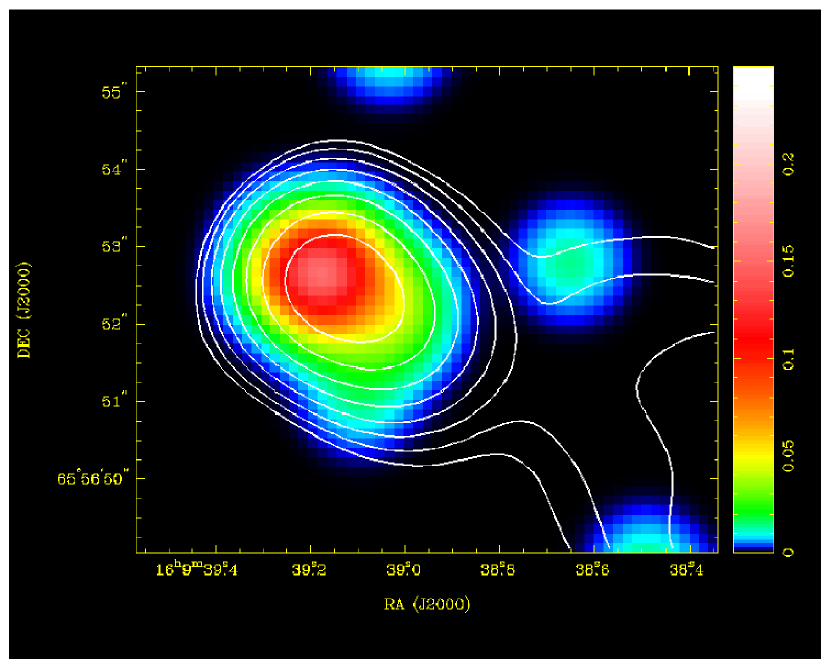
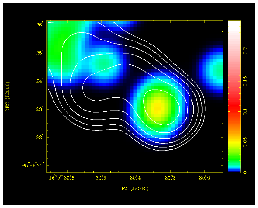
Figure 9: The X-ray hotspots of 3C 330 smoothed with a 1″ Gaussian. Contours in both cases are from an 8.4-GHz radio map with a resolution of $1\farcs 2$, approximately matched to the X-ray resolution. The contours increase logarithmically by a factor 2 and the lowest contour is at 1 mJy beam^-1. Left: NE hotspot; Right: SW hotspot.

Fig. 9 shows that the NE radio-bright hotspot of 3C 330 is clearly detected in the X-ray. There is also a weak but significant detection of the SW hotspot. The X-ray peak of the brighter hotspot agrees well with the radio flux peak, and it may be marginally extended along the same axis as the bright radio-emitting region.

There are insufficient net counts even in the brighter hotspot to extract a spectrum. We convert the count rates to 1 keV flux densities on the basis of a power-law spectrum with $\alpha_{\rm X}=0.5$ and Galactic absorption. The conversion factor is not sensitive to the precise choice of spectral index.

Neither hotspot is detected in the HST observation. We set a $3\sigma$ upper limit on each hotspot’s optical flux density of 0.5 $\mu$Jy at $5.5\times 10^{14}$ Hz.

Figure 10: The source-frame spectrum of the N hotspot of 3C 330. Radio points from Table 9, the optical HST flux density limit and the X-ray flux density are plotted together with the best-fitting synchrotron model with $\gamma_{\rm min}=1000$ (solid line) and the predicted SSC (dot-dashed line) and CMB/IC (dotted line) emission from the hotspot at equipartition. The high-energy cutoff is set to $\gamma_{\rm max}=1.4\times 10^{4}$ in this figure.

The spectrum of the NE hotspot of 3C 330 is plotted in Fig. 10. The structure of this hotspot is quite well resolved by the high-resolution image of G02; it can be modeled adequately as a cylinder with length $2\farcs 3$ and radius $0\farcs 64$ with a linear intensity gradient along its length (which we model as a linear increase in electron spectral normalization).

The spectrum of the hotspot at radio frequencies is steep ($\alpha\approx 1.0$), and, since we only have one high-resolution map and cannot resolve any spectral structure of the hotspot, we simply model it as a single broken power-law model with the break between spectral indices of 0.5 and 1.0 occurring close to 1.4 GHz. For equipartition, $\gamma_{\rm break}=3000$. We set $\gamma_{\rm min}=1000$. The best fit to the radio observations, including the high-frequency BIMA data, is well fit with a model with $\gamma_{\rm max}=1.4\times 10^{4}$; the spectral index between 15 and 85 GHz is steeper than 1.0, which requires the cutoff to be at low energies. In this model, the equipartition field strength is 9.5 nT, and the predicted SSC flux density is 0.49 nJy. If the hotspot is not in the plane of the sky, projection means that the actual long axis of the hotspot is longer than we have assumed, and the predicted SSC emissivity is reduced, by about 10% for an angle to the line of sight of 45 degrees. Given these uncertainties, we can say that the observed SSC emission in the NE hotspot, with a 1-keV flux density of $0.34\pm 0.07$ nJy on simple spectral assumptions, implies a magnetic field equal to or slightly higher than the equipartition value.

The compact component of the SW hotspot is only resolved from the others at 8 GHz, so we cannot measure its spectrum; we assume the same electron spectral values as for the NE hotspot, with a spherical model. The predicted 1-keV SSC flux density from this component at equipartition ($B=18$ nT) is then between 0.03 and 0.04 nJy, depending on the value of $\gamma_{\rm max}$. This is consistent with the observed flux density of $0.09\pm 0.04$ nJy, given the large uncertainties, but the observations are better fit with a magnetic field strength a factor $\sim 1.5$ below equipartition.

5.4 Lobes

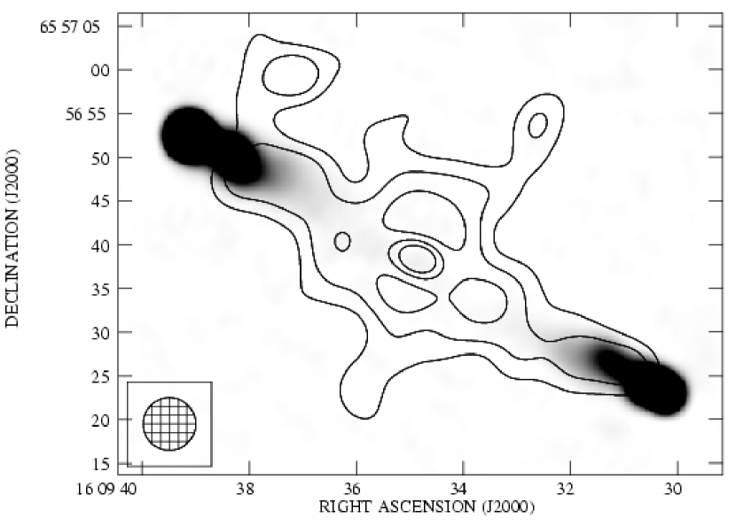
Figure 11: The lobes and extended emission of 3C 330. The contours show the X-ray emission smoothed with a 6″ (FWHM) Gaussian. The hotspot regions were masked out before smoothing and a scaled, smoothed, energy-weighted PSF model was subtracted from the image after smoothing to remove the nuclear emission. The lowest contour is the $3\sigma$ level, defined according to the prescription of Hardcastle (2000), and the contours increase logarithmically by a factor $\sqrt{2}$. The FHWM of the Gaussian used to convolve the X-ray emission is shown in the bottom left-hand corner. The object to the NW of the NE hotspot seems to be a faint background X-ray source. The greyscale shows the 8.4-GHz VLA image with 3″ resolution of G02; black is 10 mJy beam^-1.

3C 330’s lobes are both clearly detected in the X-ray (Fig. 11). We defined rectangular extraction regions which avoid the core (starting at about 10″ away from it) and the hotspots, using parallel adjacent rectangles on either side to give a local background subtraction. The lobes each contain about 20 net counts in the 0.4–7.0 keV range, so it is not possible to extract useful spectra. As with the hotspots, we convert the count rate to 1-keV flux density on the basis of a power law with $\alpha_{\rm X}=0.5$ and Galactic absorption.

We model the lobes with the same spectral assumptions as for 3C 263 (§6). In this case the predicted 1-keV flux densities from CMB/IC at equipartition are 0.17 and 0.18 nJy. Given the large errors on the measured lobe fluxes, we cannot rule out equipartition in this case; taking the measured fluxes at face value, they imply magnetic field strengths a factor $\sim 1.4$ below equipartition. These would imply internal lobe pressures from electrons and magnetic field of around $1.5\times 10^{-12}$ Pa.

5.5 Extended emission

Figure 12: Background-subtracted radial profile of 3C 330 after hotspot- and lobe-related emission has been masked out. The two light solid lines show the PSF (smaller scale) and extended model (larger scale) fitted to the source, and the heavy line is their sum.

3C 330 has weak extended emission (Fig. 12), with the fits showing evidence for only $186_{-37}^{+44}$ extended counts out to 70 arcsec (0.5 Mpc). The best-fitting $\beta$ model has $\beta=0.65_{-0.18}^{+1.3}$, $\theta_{c}=5\farcs 9_{-3.7}^{+15}$ (errors are $1\sigma$ for two interesting parameters). The luminosity of this extended component is then around $3\times 10^{43}$ ergs s^-1, corresponding to a temperature around $1.5$ keV. In the best-fitting model, the central density is $\sim 2\times 10^{4}$ m^-3 and the central pressure $8.4^{+9.1}_{-3.8}\times 10^{-12}$ Pa. The pressure at distances corresponding to the lobes, assuming little projection of this source, varies from $2.2^{+0.4}_{-0.3}\times 10^{-12}$ Pa (at $10\arcsec$, 70 kpc) to $3.3^{+1.0}_{-2.0}\times 10^{-13}$ Pa (at $30\arcsec$, 210 kpc). These are similar to the estimate of the internal lobe pressure above: the lobes would be in pressure balance at a radius of around $10\arcsec$ but could be overpressured with respect to the external medium at larger distances.

6 3C 351

6.1 Introduction

3C 351 is a well-studied $z=0.37$ quasar. Radio images have been presented by Leahy & Perley (1991), B94, and G02; their most striking feature is the bright double hotspot pair to the N and the displaced nature of the N lobe. The hotspots are also detected in the optical (Röser, 1989; Lähteenmäki & Valtaoja, 1999). The X-ray emission from the bright nucleus has been extensively studied (Fiore et al., 1993; Mathur et al., 1994; Nicastro et al., 1999) and it has been argued that the unusual X-ray spectrum seen in ROSAT PSPC data is due to an ionized absorber, often seen in Seyfert 1 galaxies but a rare feature in quasars. No extended X-ray emission was detected with ROSAT (Hardcastle & Worrall, 1999), but the hotspots were seen in a short Chandra observation (Brunetti et al., 2001).

6.2 Core

Figure 13: X-ray spectrum of 3C 351 nucleus. Left: the spectrum with the best-fitting two-power-law model. Right: the spectrum with the best-fitting ionized-absorber model. The lower panels show the contributions to $\chi^{2}$, plotted with the sign of the residual.

The X-ray centroid, using the default Chandra astrometry, is at $17^{\rm h}04^{\rm m}41\fs 326$, $+60\arcdeg 44^{\prime}30\farcs 22$. 3C 351’s radio core contains two compact components of similar 8-GHz flux density separated by $0\farcs 35$. B94 and G02 both argue that the southern component is the true core, while the northern component is a jet knot. The radio position of the southern component, using the 8-GHz radio map of G02, is $17^{\rm h}04^{\rm m}41\fs 364$, $+60\arcdeg 44^{\prime}30\farcs 46$. This is in good agreement with the position given by B94 and implies a radio-X-ray misalignment of $0\farcs 37$. We shift the X-ray data to align the X-ray core with the southern radio component. However, it is possible that some of the X-ray emission observed from the core region comes from the northern radio component, since the two components would not be well resolved by Chandra. We see no evidence for extended emission from the X-ray core, and no difference between the core centroids in different X-ray energy ranges, but the possibility means that the alignment of the radio and X-ray frames is less secure than it would otherwise be.

We obtain many counts in the X-ray core, and so detailed spectroscopic analysis is possible. Unsurprisingly, in view of previous work, a single power-law model with Galactic absorption is an unacceptable fit to our data ($\chi^{2}/n=638/215$, where $n$ denotes degrees of freedom); we see strong residuals at 0.6–0.8 keV. A two-power-law model, with one of the power-law components having additional intrinsic absorption (as used above for 3C 330) is a better fit, with $\chi^{2}/n=304/212$ and an intrinsic cold absorbing column of $(1.1\pm 0.1)\times 10^{22}$ cm^-2; but the best-fitting spectral index of the unabsorbed component in this model is well constrained and steep, $\alpha=2.5\pm 0.3$. The absorbed power law has $\alpha=0.46\pm 0.05$. This model is plotted in Fig. 13. If the absorbed component is associated with the active nucleus and the unabsorbed component with the radio emission, then the absorbing column, which represents only 2 magnitudes of visual extinction, is small enough to be compatible with the predictions for a quasar within unified models, while the 1-keV flux density of the unabsorbed component would be 14 nJy, which is consistent with the radio-X-ray relation of Hardcastle & Worrall (1999).

We fit two alternative models, consisting of a single power law with Galactic absorption plus either ‘windowed’ absorption (the zwndabs model in xspec), which roughly mimics a warm absorber, or the xspec ionized absorber model (absori). The zwndabs model gives a less good fit than the power-law models, with $\chi^{2}/n=344/213$; it has a window energy (source-frame) of $0.78\pm 0.01$ keV and an absorbing column of $(3.7\pm 0.2)\times 10^{21}$ cm^-2, and the best-fitting power-law index is very flat ($\alpha=0.10\pm 0.02$). The ionized absorber model gives a slightly better fit, $\chi^{2}=322/213$, with the ionizing continuum power-law index fixed to $\alpha_{i}=0.5$, the absorber temperature set to $3\times 10^{4}$ K and the iron abundance set to unity. In this model, shown in Fig. 13, the power-law index $\alpha=0.42\pm 0.04$, the absorbing $N_{\rm H}=(1.5\pm 0.1)\times 10^{22}$ cm^-2, and the ionization parameter $\xi=34\pm 5$ ergs cm^-1. This absorbing column is consistent with the value obtained (under a slightly different model) by Nicastro et al. (1999).

None of these models is a particularly good fit to the data, with particularly strong scatter about the models to be seen below 0.6 keV (Fig. 13). In Table 8 we tabulate the results for the two-power-law models, as they remain formally the best fits. Two weak line-like features are seen in the spectrum, at observed energies of about 3.2 and 4.7 keV (Fig. 13). When these are fit with Gaussian models, the first feature’s width is not well constrained, and it is best fitted with very broad lines. This reduces our confidence in its physical reality as an emission feature. The second feature can be modeled as a Gaussian with rest-frame energy $6.40\pm 0.07$ keV and $\sigma=70\pm 70$ eV, with equivalent width 70 eV. The improvement to the fit of adding this feature is very limited, but given its energy it may be a marginal detection of the iron K$\alpha$ line.

6.3 Hotspots

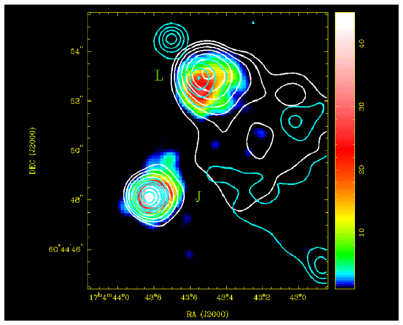
Figure 14: 3C 351 X-ray hotspots. The Chandra data are smoothed with an $0\farcs 5$ Gaussian. The white contours are 8.4-GHz radio contours with a resolution of $0\farcs 85$, approximately matched to the X-ray resolution. The contours increase logarithmically by a factor 2 and the lowest contour is at 0.25 mJy beam^-1. The light blue contours are the HST $R$-band data at the same resolution, and also increase logarithmically by a factor 2 (arbitrary units). The structure in the bottom right of the image is due to noise on the HST PC chip.

As previously reported by Brunetti et al. (2001), both of the northern hotspots of 3C 351 are detected in the X-ray (Fig. 14); the compact ‘primary’ hotspot J and the diffuse ‘secondary’ hotspot L (using the notation of B94). In our observations five times more counts are obtained than in the dataset used by Brunetti et al., giving us well-constrained hotspot spectra (Table  8). We obtain 1-keV flux densities and spectral indices that agree with the values determined by Brunetti et al. within the joint $1\sigma$ uncertainties.

When these hotspots are compared with a radio map (Fig. 14) there is a clear offset of about 1″ between the X-ray and radio peaks in the secondary hotspot L, in the sense that the distance between the peaks of J and L is smaller in the X-ray than in the radio. L appears to be resolved by Chandra and to be comparable in size to its radio counterpart ($\sim 2^{\prime\prime}$). There is no clear colour gradient in the X-ray images of L, and no obvious radio spectral index gradient at high frequency. There is an extension of J to the north with no radio counterpart, but it is otherwise not resolved by Chandra.

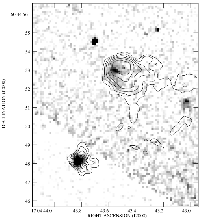
Figure 15: 3C 351 optical hotspots at the full HST resolution. The HST data are shifted so that the positions of hotspot J align in the optical and radio. The contours are from an 8.4-GHz radio map at $0\farcs 34\times 0\farcs 23$ resolution. The WFC chip lies in the bottom left of this image, the PC chip in the top right.

Optical counterparts to both northern hotspots in 3C 351 were discovered by Röser (1989) and their relationship to the radio emission confirmed by Lähteenmäki & Valtaoja (1999). Further optical observations were made by Brunetti et al. (2001), who also discuss the HST observations that we use in this paper. When the HST observations are compared with high-resolution radio maps, it appears that the optical counterpart of hotspot L may be offset from the radio peak in the same sense as is seen in the X-ray (Figs 14 and 15). The two optical hotspots unfortunately lie on different chips of the HST WFPC2, and there are no reference sources in the PC chip to tie the radio and optical frames together. Significant offsets are present using the default HST astrometry, as expected. The evidence for an offset relies on the accuracy of the wmosaic task in the STSDAS package in iraf, used to produce the mosaiced image shown in these Figures. However, the size of the offset ($0\farcs 5$) seems too large to be accounted for by uncertainties in the WFPC2 chip geometry; other sources which span chip boundaries in this field (notably some faint galaxies near the quasar nucleus) do so without showing any evidence for such offsets. We conclude that the observed offset may well be real. In this case, the optical peak of L lies between the radio and X-ray peaks.

We agree, within the errors, with the HST R-band flux density measured by Brunetti et al. (2001) for hotspot J. However, we obtain a substantially lower flux density for hotspot L, although the errors are comparatively large because of uncertainties in background subtraction. We adopt flux densities of $2.4\pm 0.1$ $\mu$Jy and $1.9\pm 0.2$ $\mu$Jy for J and L respectively.

Figure 16: The source-frame spectra of the N hotspots of 3C 351: left is hotspot J and right is hotspot L. Radio points from Table 9, the R-band HST flux densities determined by us, the ground-based B-band flux densities of Brunetti et al. (2001) and the X-ray flux densities and spectra are plotted together with the synchrotron models discussed in the text (solid line) and the predicted SSC (dot-dashed line) and CMB/IC (dotted line) emission from the hotspot at equipartition. The high-energy cutoff is set to $\gamma_{\rm max}=1.3\times 10^{6}$ in this figure.

The compact hotspot of 3C 351 (J) is not well resolved at any radio frequency available to us, and is compact even in the HST images. The size derived from fitting a homogeneous sphere model depends on the frequency and resolution of the data used, suggesting that there may be unresolved spatial or spectral structure. The value we adopt ($r=0\farcs 16$) is based on fitting a homogeneous sphere model to the 8.4-GHz data of G02. This is larger than the value used by Brunetti et al. (2001), who just took half the FWHM of the Gaussian fit of B94. Spectrally, the hotspot seems to have a steeper spectrum between 1.4 and 8 GHz than between 8 and 15 GHz, but this may be due to contamination from more extended emission in the low-resolution 1.4-GHz map; the maps of B94 and G02 both show structure around this hotspot. The high-frequency (15-85 GHz) spectral index of the hotspot is close to 1.0. If we assume that some of the 1.4-GHz flux density is not from the compact region, then the 8.4, 15 and 85-GHz and optical data points can be fit, though not particularly well, with a version of our standard spectral model, in which the synchrotron spectral index steepens from 0.5 to 1.0 in the radio, and then retains this value out to beyond the B-band. Since the optical to X-ray spectral index is close to 1.0, the 1-keV X-ray data point alone can then be fit as an extension of the synchrotron spectrum, with $\gamma_{\rm max}>6\times 10^{7}$ at equipartition (this conclusion differs from that of Brunetti et al., who find a somewhat lower maximum contribution from synchrotron emission, because of the steeper injection index they use). However, the flat X-ray spectrum of the hotspot ($\alpha_{\rm X}=0.5\pm 0.1$) is inconsistent with a synchrotron model. Like Brunetti et al., we prefer a synchrotron model in which the break is at higher frequencies and the synchrotron emission is cutting off in the optical ($\gamma_{\rm break}=5800$, $\gamma_{\rm max}=1.3\times 10^{6}$ at equipartition). This improves the fit to the radio and optical data. However, in this model, plotted in Fig. 16, the predicted inverse-Compton flux density at equipartition ($B_{\rm eq}$ = 21 nT) is 55 pJy, almost two orders of magnitude below the observed value. The magnetic field must be reduced by a factor $\sim 12$, to 1.7 nT, to produce the observed emission from the SSC process. In this case $\gamma_{\rm max}=4.8\times 10^{6}$, $\gamma_{\rm break}=2.0\times 10^{4}$, and the predicted X-ray spectral index at 1 keV is 0.6, close to the observed value.

Hotspot L is well resolved in the radio and HST images. A direct measurement on the radio map shown in Fig. 14 gives dimensions for the bright region of about $2\farcs 2\times 1\farcs 6$. No simple geometrical model is a good fit to the structure of this hotspot, with its off-center brightness peak and filamentary extensions to the SW. We begin by treating the brightest part of the hotspot as a homogeneous sphere with $r=0\farcs 8$; this radius agrees both with the high-resolution measurements and with fits to the low-resolution 1.4 and 15-GHz maps, but is again somewhat larger than that used by Brunetti et al.. The radio and optical data can then be fit with a spectral model very similar to that used for hotspot J; the 1.4-GHz data point again lies above the extrapolation of the spectrum inferred from the high-frequency radio data, but neglecting this, we find very similar break and cutoff values, $\gamma_{\rm break}=8400$, $\gamma_{\rm max}=1.3\times 10^{6}$, at equipartition ($B_{\rm eq}=7.1$ nT). This model is plotted in Fig. 16. If the X-ray emission is SSC, the predicted inverse-Compton flux density in this model is 80 pJy, and the magnetic field strength would have to be reduced by a factor $\sim 9$, to 0.8 nT, to produce all the observed emission by the inverse-Compton process. The predicted 1-keV X-ray spectral index in this model is also 0.6, which is somewhat flatter than the observed value of $0.85\pm 0.1$.

The inverse-Compton model cannot explain the observed offsets between the X-ray and radio centroids of hotspot L. To explain this offset while retaining a simple model of the electron distribution we would need an external illuminating source, but no such source is apparent; in particular, hotspot J is much too far away to produce a significant effect (the predicted flux density from IC scattering of J’s photons by L is only 2 pJy at equipartition, or 2% of the predicted SSC flux density). Otherwise, if the X-rays are to be SSC emission, there must be significant electron spectral structure in the hotspot which we have failed to take into account in our model. With only one high-resolution, high-frequency radio map, it is impossible to test this suggestion, but the possible offset seen between the radio and optical positions may support it.

Unlike Brunetti et al., because of the lower R-band optical flux density we obtain, we find 3C 351 L to have a relatively flat optical spectral index, $\alpha_{\rm O}\approx 0.8$ (similar to the X-ray spectral index), and this means that a synchrotron model connecting the optical and X-ray emission cannot be ruled out in this hotspot either, and is an alternative explanation for the bright X-ray emission, though it would require a second, flat-spectrum synchrotron component to be present.

The differences we find between the equipartition/minimum energy and SSC fields in these two hotspots are larger than the factor $\sim 3$ inferred by Brunetti et al. (2001) because of differences in our assumptions. As noted above, we use larger angular sizes for the hotspots, and this accounts for a substantial part of the difference. Brunetti et al. used a different definition of the minimum energy, obtaining a lower field strength than our calculation would have given on the same assumptions about hotspot size. They also used a version of the more complex electron energy spectrum described by Brunetti et al. (2002a). This illustrates a general point: differences in model parameters can have an important effect on the derived magnetic field strength.

The weak S radio hotspot of 3C 351 is not detected in the X-ray. Based on the background count rate around the hotspot region, we can set an upper limit on its X-ray flux density (Table 8). It does not lie in any of the HST fields, so no optical upper limit is available, and we do not have enough high-resolution data to comment on its radio spectrum. In the 8-GHz maps it is resolved into two components, with flux densities of 2.2 mJy and 1.1 mJy. Both components are extended. Using a spectral model similar to that used for hotspot J, we find that the two components of A taken together would have an SSC flux density of approximately 0.2 pJy, a factor 250 below our upper limit. Thus, even if these hotspots were brighter than their equipartition flux density by the same factor as hotspot J, we would not have detected them in our observations. We infer the weak constraint $B\gtrsim 0.04B_{\rm eq}$.

6.4 Lobes

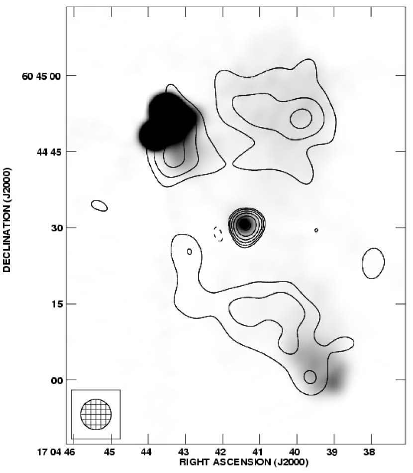
Figure 17: The lobes of 3C 351. The contours show the X-ray emission smoothed with a 6″ (FWHM) Gaussian. The hotspot regions and background X-ray point sources were masked out before smoothing (some extended emission is present around the hotspots and gives rise to the contours near them) and a scaled, smoothed, energy-weighted PSF model was subtracted from the image after smoothing to remove the nuclear emission. A narrow peak at the core position shows that the PSF model is slighly broader than the real data. The lowest contour is the $3\sigma$ level, defined according to the prescription of Hardcastle (2000), and the contours increase logarithmically by a factor $\sqrt{2}$. Negative contours (illustrating the residuals due to core subtraction) are dashed. The FWHM of the convolving Gaussian is shown in the bottom left of the image. The greyscale shows the 8.4-GHz VLA image with 3″ resolution of G02; black is 10 mJy beam^-1.

Both lobes of 3C 351 are detected with Chandra (Fig. 17). To extract spectra, we used two circular regions at identical distances (25″) from the nucleus, centered on the lobe emission, and a matched off-source background region in a suitable position angle. There are 60 net counts in the northern lobe and 40 in the southern lobe; this is insufficient for spectral analysis of either lobe alone but allowed us to fit a model to the combined emission from both (Table 8).

Modeling the lobes as described above for 3C 263 and 3C 330, we find a predicted 1-keV flux density for the CMB/IC process of 0.21 nJy for the N lobe and 0.17 nJy for the S lobe, respectively factors $\sim 5$ and $\sim 4$ below what is observed. If the X-ray emission from these lobes is to be produced by the CMB/IC process, the magnetic field strength must be a factor 2–2.5 below equipartition. The pressures in the lobes are then $\sim 4\times 10^{-13}$ Pa.

6.5 Extended emission

There is no evidence for extended, cluster-related X-ray emission in 3C 351. No additional extended model that we have fitted improves the fitting statistic significantly, and the best-fitting models contain only a few tens of counts. If we take these as very rough upper limits, the X-ray luminosity of 3C 351’s environment is no more than a few $\times 10^{42}$ ergs s^-1 (depending on choice of temperature and abundance), a group environment at best. Other evidence, such as galaxy count studies (e.g., Harvanek et al., 2001), suggests that 3C 351’s environment is poor, so this is not a surprising conclusion. The gas in groups of galaxies of this sort of luminosity can have a pressure at 100-kpc radii comparable to that estimated above for the lobes of 3C 351, so it remains possible that 3C 351’s lobes are pressure-confined by a faint X-ray emitting environment.

7 Discussion

7.1 Evidence for and against equipartition in hotspots

Table 10: The ratio between equipartition and inferred field strengths in hotspots and lobes

Source	$B_{\rm eq}/B$
	N hotspot	S hotspot	N lobe	S lobe
3C 263	$<4$	$1.9\pm 0.1$	$2.0\pm 0.3$	$2.0\pm 0.4$
3C 330	$1.0\pm 0.1$	$1.5\pm 0.4$	$1.4\pm 0.3$	$1.4\pm 0.3$
3C 351	$12\pm 0.05$	$<25$	$2.5\pm 0.4$	$2.0\pm 0.5$

Note. — For 3C 351, hotspot J is used. Errors are based on the statistical errors on 1-keV flux density quoted in Table 8, and do not include systematic uncertainties in the modelling.

The inferred field strengths, relative to the equipartition values, of the hotspots of the target sources are listed in Table 10. Of the three sources, one (3C 330) has hotspots whose X-ray emission is consistent with SSC emission at equipartition, one (3C 263) has an inferred hotspot magnetic field strength a factor 2 below the equipartition value (consistent with other sources, such as 3C 295, which show a similar deviation from equipartition) and one (3C 351) has hotspots whose X-ray emission, if it were of SSC origin, would imply a magnetic field strength an order of magnitude below the equipartition value.

What process is responsible for the anomalously bright, flat-spectrum hotspots in 3C 351? We can consider several classes of explanation. The first involves retaining the SSC process, with some modifications; the second involves invoking relativistic beaming, an idea supported by the observation of very bright, one-sided radio hotspots on the jet side of 3C 351 and by the displacement of the hotspots with respect to the radio lobe; and the third involves some emission mechanism other than the inverse-Compton process. We discuss several variants of these models in turn.

• SSC with standard electron spectral model, $B\ll B_{\rm eq}$. As discussed above, this model does not explain the offsets between the radio and X-ray peaks in hotspot L.

• SSC with standard electron spectral model, $B\ll B_{\rm eq}$, and spatial variation of the electron population. This model can explain the offsets between the peaks in various wavebands, at the cost of introducing new features in the electron population for which there is no independent observational evidence.

• SSC with second electron population, $B\sim B_{\rm eq}$. If we introduce an additional population of low-energy electrons whose synchrotron emission is below the observed radio band, , we can greatly increase the SSC flux. If we also allow this population to be offset with respect to the radio-emitting population, we can explain the properties of hotspot L. This model has the same disadvantages as 1b.

• SSC with relativistic beaming, $B\sim B_{\rm eq}$. Beaming would mean that our estimate of the hotspot flux density would not correspond to the source-frame value. The predicted SSC flux density and the ratio $B_{\rm eq}/B$ depend on the Doppler factor $\cal D$ (${\cal D}=[\Gamma(1-\beta\cos\theta)]^{-1}$ for a hotspot, where $\theta$ is the angle to the line of sight and $\Gamma=(1-\beta^{2})^{-1/2}$ is the bulk Lorentz factor). Beaming causes the observed flux densities to change by a factor ${\cal D}^{(3+\alpha)}$. For a pure power-law spectrum with electron energy index $p$ ($\alpha=(p-1)/2$), neglecting aberration effects, the predicted SSC flux can be shown to go as ${\cal D}^{-12/(p+5)}$, and so, for values of $p$ in the range 2–3, Doppler boosting, (${\cal D}>1$) reduces the predicted equipartition flux while Doppler dimming (${\cal D}<1$) increases it. To place 3C 351 at equipartition we would require $\beta\gtrsim 0.999$ ($\Gamma\gtrsim 20$) with the source lying close to the plane of the sky. This is clearly not a plausible model for a quasar; in addition, the rest-frame radio luminosity of the hotspot becomes very large.

• Boosted CMB, $B\sim B_{\rm eq}$. Relativistic fluid speeds in or close to the hotspot would give rise to an increased contribution from inverse-Compton scattering of the microwave background, which is negligible in all our sources if relativistic effects are not present. The effective energy density in microwave background photons increases as $\sim\Gamma^{2}$ (e.g., Dermer & Schlickeiser, 1993), but this is partly offset by the reduction in the electron number density. There are additional corrections because of the anisotropic nature of the inverse-Compton process; the net result is that a source exhibiting emission from this process must be close to the line of sight. Because of the blueshifting of the CMB photons in the source frame, the results are also strongly dependent on the presence of low-energy electrons; in order to obtain a spectrum which is not flat or inverted, we require, approximately, $2\times 10^{-7}(1+z)\gamma^{2}_{\min}\Gamma^{2}\ll 1$. To reproduce the observed emission from 3C 351 with an equipartition $B$-field and the lowest possible bulk $\Gamma$, $\Gamma\sim 5$, we require $\gamma_{\rm min}\sim 10$ and $\theta=0\arcdeg$. Larger angles to the line of sight require larger $\Gamma$ values. This model thus requires 3C 351 to be very close to the line of sight (for $5<\Gamma<20$, $\theta\lesssim 6\arcdeg$, so the linear size of the source would have to be $\gtrsim 4$ Mpc, if bending is neglected). We also require highly relativistic flows to power both J and L: either the jet splits, or (more conventionally) a relativistic outflow from J powers L. In the second case, we would expect $\Gamma$ to be different in the two hotspots. The angles between the line of sight and the velocity vectors of the flows powering the hotspots are likely to differ in either situation, because the hotspots and the core do not lie on a straight line: so in this model the parameters must ‘conspire’ to ensure that the X-ray to radio ratios remain similar in the two hotspots. This model does not explain the offsets in hotspot L without some additional assumptions, such as finely tuned velocity vector variations in the hotspot.

• Boosted CMB, but hotspots are ‘jet knots’, $B\sim B_{\rm eq}$. In this model, the objects we have described as hotspots are not terminal hotspots at all, but knots in a projected jet (which presumably terminates somewhere else (e.g., in the displaced N lobe) in a hotspot of brightness comparable to that in the S lobe. This model has the advantage that we do not (necessarily) expect jet deceleration between knots, and that it allows us to retain sub-relativistic speeds in the hotspots. Otherwise it has the same disadvantages as 2a.

• Boosted hotspot back-scattering, $B$ unknown. We cannot rule out the possibility that the X-ray emission does not originate in the hotspot (post-shock) region at all. It could instead be due to scattering of hotspot photons by the incoming, presumably highly relativistic jet. This model has the advantage that it can explain the offsets observed in hotspot L. It has the disadvantage that, as no radio jets are observed entering the hotspot, we cannot use the observations to constrain magnetic fields or jet speeds. Because the IC emission from this process is even more anisotropic than for 2a and 2b, the problem of the angle made by the jet to the line of sight becomes greater in this model.

• Synchrotron from second electron population, $B$ unknown. A second, flat-spectrum synchrotron component in the X-ray (and possibly also the optical) can explain many of the observations of 3C 351’s hotspots, including the offsets seen in hotspot L if the second electron population is spatially offset from the low-energy electrons responsible for the radio emission. Given the very different loss timescales in the radio and X-ray, and the rapidly changing nature of hotspots (and the bulk flows that feed them) that numerical simulations suggest, there is no very strong reason to believe that a single electron energy power law should describe observations made at a given moment, so a picture of this kind is not inconsistent with standard models of radio sources. The X-ray emission in the jets of certain sources, such as 3C 120 (Harris et al., 1999) and 3C 273 (Jester et al., 2002), has been explained in terms of a model of this kind.

• Synchrotron from second electron population and SSC, $B$ unknown but $B\sim B_{\rm eq}$ permitted. This is a trivial variation on model 3a in which some of the X-ray emission is due to SSC rather than synchrotron.

• Proton-induced cascade or other exotica, $B$ unknown. As usual, we cannot rule out the possibility that some less familiar emission process makes a contribution to the X-ray emission.

All these models are ad hoc in one way or another. The beaming models do help to explain the large-scale asymmetry of the radio source as well as the X-ray emission, but they all require 3C 351 to be very close to the line of sight and extremely large in unprojected linear size, as well as invoking speeds in the hotspot regions that are very much higher than have been inferred from other work. The other models require less extreme parameters for the radio source, but do not answer the question of why 3C 351 is unlike the other sources in the sample, which show no evidence for strong departures from equipartition, extra electron populations, or new emission mechanisms.

It is interesting to compare the results on 3C 351 with those on other FRII sources with ‘bright’ X-ray hotspots, such as Pictor A and 3C 390.3. In the case of Pictor A, Wilson, Young & Shopbell (2001) found that a magnetic field a factor 14 below the equipartition value would reproduce the flux density of the X-ray hotspot, but they reject a simple SSC model of the type we have used in this paper because of the well-constrained steep spectrum of the hotspot ($\alpha_{\rm X}=1.07\pm 0.11$). A simple synchrotron model is also rejected because the optical data require a cutoff in the optical (Meisenheimer, Yates & Röser, 1997). However, Wilson et al. do not rule out a model in which there are contributions from both X-ray synchrotron and SSC emission, as in model 3b above, which requires $B_{eq}/B\approx 9$. This factor is similar to those that we would require in 3C 351 on the pure SSC model (1a). They also consider the possibility of a second electron population (models 1c and 3a above).

In the case of 3C 390.3, Harris et al. (1998) rejected a SSC model for the ROSAT-detected X-ray hotspot, hotspot B, because the X-ray emission was much brighter than their SSC prediction. The Chandra observation of this source (Wagner et al., in preparation) detects all three compact hotspots in 3C 390.3 and allows a more precise determination of some of the source parameters. Examining the archive data, we find that the brightest hotspot, hotspot B, has a 1-keV flux density of $4.5\pm 0.3$ nJy, in good agreement with the result of Harris et al., and $\alpha_{\rm X}=0.88\pm 0.17$. The radio, optical and X-ray data in hotspot B can be connected with a simple synchrotron model. An SSC model requires a large departure from equipartition; with our cosmology and standard spectral assumptions we find $B_{\rm eq}/B\approx 90$, much higher than in any other source we have examined. Moreover, the predicted SSC spectral index is $\sim 0.5$, while the spectral index in the synchrotron model is $\sim 1.0$, so that the Chandra spectrum favors the synchrotron model. We see no reason to believe that there is a significant contribution from SSC emission in hotspot B of 3C 390.3. The Chandra spectra of the two other X-ray detected hotspots in 3C 390.3 are even steeper than in hotspot B, which suggests that a synchrotron model is required there as well. It seems likely that the differences between the radio to X-ray spectra of the three hotspots, remarked on by Harris et al., can be explained in terms of similar electron spectra with different high-energy cutoffs. Given the large number of jets in low-power radio galaxies now thought to be due to synchrotron radiation (§1), the existence of the required high-energy electrons in hotspots is no longer as remarkable as it once seemed. This observational evidence for synchrotron emission in hotspots is indirect support for one of the synchrotron models (3a/b above) to explain the emission from 3C 351.

The Chandra data on hotspots in general are therefore reinforcing the conclusion, already suggested by ROSAT observations, that more than one emission mechanism is operating in the X-ray in FRII hotspots. Some hotspots, of which 3C 390.3 is to date the most convincing example, require an X-ray synchrotron model. Some, such as Cygnus A, 3C 123, 3C 263 and 3C 330, are likely to be pure SSC, with no significant contribution to the X-rays from synchrotron emission and a hotspot magnetic field close to the equipartition value. And some, such as Pictor A and perhaps 3C 351 (model 3b above), may have synchrotron and SSC emission at similar levels, or may be different from the other sources in some more interesting way. In order to distinguish between these cases, good radio and optical information and, ideally, an X-ray spectrum of the hotspot are required: further high-resolution observations in the radio, optical and UV may be required to to disentangle the emission mechanisms in Pictor A and 3C 351.

In this picture, the questions remaining to be answered are:

• What is special about the hotspots that exhibit X-ray synchrotron emission? It’s particularly striking that all three compact hotspots of 3C 390.3 are X-ray synchrotron emitters, despite being quite different in their local environments and radio structures (see Leahy & Perley, 1995). There is no obvious way in which these hotspots, in quite different parts of the source, can ‘know’ that they should accelerate electrons to high energies — unless some intrinsic property of the beam is involved.

• What is special about the hotspots, like 3C 351 and possibly Pictor A, that may have $B_{\rm eq}/B\gg 1$?

Brunetti et al. (2001) suggested a partial answer to the second of these questions. They pointed out that, in standard shock-acceleration models, the high-energy cutoff of the synchrotron electron population is higher for lower hotspot magnetic fields, because it is determined by the balance between acceleration and synchrotron loss processes. In other words, we might expect to see an enhanced contribution from SSC emission in radio sources which we know by other means to have a synchrotron spectrum extending to high energies. This might apply to 3C 351 and Pictor A, which are known to have optical synchrotron hotspots, while sources like Cygnus A and 3C 123, whose electron spectra are known to cut off at lower energies, have fields closer to equipartition. However, one source in the current sample, 3C 263, breaks the trend by having an optical synchrotron hotspot without being particularly X-ray bright. And this picture does not explain why it is that some sources have particularly low hotspot B-fields, or why, in the case of 3C 351, both hotspots appear to do so.

Numerical simulations (e.g., Tregillis, Jones & Ryu, 2001) lead us to expect that hotspots will be transient structures, and may well have different magnetic field and electron acceleration behaviour at different times. All hotspots may pass through phases of inverse-Compton domination and synchrotron domination of their X-ray output. If this is the case, neglecting the probably important question of observational bias, then the statistics of detected sources are telling us that sources spend approximately equal times in the two regimes. However, this does not explain (and is even to some extent incompatible with) the observation of correlated properties in spatially separated hotspots, as observed in Cygnus A, 3C 351 and 3C 390.3.

7.2 Inverse-Compton emission from lobes? Constraints on lobe physics

Both lobes of all three sources are detected in the X-ray. In all three cases, the measured X-ray emission is close to the predicted value for inverse-Compton scattering of CMB photons, requiring field strengths which are factors between 1.4 and 2.5 below equipartition values on simple models which treat the lobes as uniform (Table 10). We have not taken into account any possible illumination of the lobes by the quasar nuclei (nuclear inverse-Compton, NIC), which would give an additional photon contribution and reduce the discrepancy between the inferred and equipartition magnetic field strengths. We do not believe that nuclear illumination is likely to dominate the CMB photon field in our sources, since in 3C 263 and 3C 351 there is no evidence for a higher ratio of X-ray to radio flux in the lobes on the counterjet side, as would be expected, due to the anisotropy of the inverse-Compton process, in a NIC model (Brunetti et al., 1997).

Is the lobe emission inverse-Compton in origin at all? The similarity of the observed fluxes to the predicted values, and the tight relationship between the emitting regions in radio and X-ray, suggest this, but cannot confirm it. The X-ray spectra are not good enough in any of our sources to allow us to rule out a thermal origin for the lobe emission, although the existence of some hard counts (e.g., in 3C 263’s N lobe and 3C 351) would imply quite high temperatures, $kT\sim 5$ keV). If the X-rays were thermal, their spatial similarity to the radio emission means that they would have to originate either inside the lobes, or in a boundary layer around the lobes with a thickness considerably less than the lobe dimensions (i.e., no more than a few kpc, given the spatial resolution of Chandra). Polarization observations are conventionally taken to rule out the presence of large amounts of thermal material inside radio lobes, although, as pointed out by Laing (1984), large amounts of thermal material can be hidden by suitable magnetic field configurations. Unfortunately, estimates of the depolarization measure $DP$ are not available to us for either of our quasars. For 3C 330, Fernini (2001) quotes values of $DP$ (the ratio of polarization at two frequencies, in this case 1.4 and 5 GHz) of 0.84 and 0.55 for the two lobes. (A lower $DP$ means more depolarization.) We can convert the observed Chandra count rate for the lobes of 3C 330 into a thermal proton density using xspec and assuming that the thermal plasma uniformly fills the radio lobes; we use a mekal model with $kT=5$ keV, $0.3$ solar abundance and Galactic absorption. We find that a thermal proton density of $\sim 10^{4}$ m^-3 would be required. Using equipartition fields, this would give rise to a large Faraday depth, and, using the results of Cioffi & Jones (1980), we would expect $DP\sim 0.08$, which is much less than the observed value; we would also expect a very low degree of polarization at low frequencies, whereas we know that the source remains polarized at 1.4 GHz. We cannot reduce the Faraday depth by significantly decreasing the assumed magnetic field strength, as the X-ray observations set a lower limit on the field strength, $B>B_{\rm eq}/1.5$. So, for simple field geometries, the idea that thermal protons are inside the lobes is not consistent with the radio data.

If the thermal protons are instead in a boundary layer of shocked gas around the source, their density can be estimated in the same way, and is greater than the value calculated above by the square root of the ratio of the boundary layer to source volumes: for example, if the boundary layer were $0\farcs 5$ (3.5 kpc) thick in 3C 330, the density would be higher by a factor $\sim 1.5$. Here Faraday-rotation constraints are less helpful, because we do not know the value of the external magnetic field strength. However, if the external thermal material is assumed to be shocked ambient gas, well-known results for the density contrast in a shock imply that the ambient gas density must be no more than a factor 4 less dense than the inferred external density, or at least a few $\times 10^{3}$ m^-3. This is comparable to, though on average somewhat larger than, the density of the external material inferred from the observations described in §12 at the distance of the lobes of 3C 330, so this model remains possible from that perspective. However, it seems likely that this external gas is too hot (particularly in 3C 263) to give rise to the observed X-ray emission when shocked, unless the shocks are only weak (in which case the stand-off distance needs to be large). There is also no obvious gradient of X-ray emissivity along the sources, particularly 3C 330, although the $\beta$-model fits of §12 imply that the external density drops by an order of magnitude along the length of the lobes in that source. And there is no evidence in the X-ray data of the limb-brightening expected in such a model, although the small number of counts from the lobes makes detailed analysis of the lobe structure difficult. We conclude that, although models in which the lobe-related X-ray emission are due to an external boundary layer are not ruled out, they are more contrived than the alternative of an inverse-Compton origin with a magnetic field somewhat lower than the equipartition value.

Whether or not the emission is inverse-Compton in origin, its detection places some interesting constraints on the filling factors in the lobes, by giving an upper limit on lobe X-ray emissivity. As pointed out by Hardcastle & Worrall (2000), the dependence of inverse-Compton emissivity on filling factor is complicated, depending on the nature of the ‘fluid’ that fills the gaps between radio-emitting regions. However, if the fluid is relativistic electrons, i.e., the lobes consist of a more or less uniform distribution of electrons with a very wide range in magnetic field strengths, then the inverse-Compton emissivity increases as the filling factor $\phi$ decreases. In the simple case in which the magnetic field is either on or off, and where on is in energy equipartition with the synchrotron-emitting electrons, the IC emissivity over the entire lobe goes up approximately as $\phi^{-4/7}$. This sort of model is constrained by the observations to have $\phi\gtrsim 0.1$. The constraint is difficult to evade if we require that there are no strong pressure differences in the lobes. Filling factors lower than this are only possible if the non-radiating ‘fluid’ does not consist of electrons — for example, if the magnetic field dominates the overall energy of the lobes. We note that less extreme models with inhomogenous magnetic field distributions are not ruled out by the data. For example, the models used by Tribble (1991) give only a modest increase ($\sim 20$%) in the expected inverse-Compton emissivity if the mean field energy is in equipartition with the electrons.

A CMB inverse-Compton model, and the inferred relatively small but non-zero departures from equipartition, are consistent with early observations of less powerful sources with ROSAT and ASCA (e.g., Feigelson et al., 1995; Tsakiris et al., 1996; Tashiro et al., 1998) as well as with new results now emerging from Chandra observations of sources more similar to our targets (Brunetti et al., 2002a, b; Fabian, Celotti & Johnstone, 2002).

7.3 Thermal emission and pressure balance

The extended emission around 3C 263 and 3C 330 seems very likely to be thermal emission from a cluster-scale atmosphere: we have thus confirmed earlier predictions (Hall et al., 1995) that 3C 263 should lie in an X-ray emitting cluster. If the lobe X-rays are indeed inverse-Compton emission, the model we favor of those discussed in §7.2 above, then the required departures from equipartition produce lobe pressures which are consistent, within the uncertainties on the various calculations, with the inferred external pressures. Small departures from equipartition may therefore solve the problem, discussed by Hardcastle & Worrall (2000), of the apparent under-pressuring of the radio lobes with respect to the external medium; this is particularly true if some of the X-ray emission detected by Hardcastle & Worrall with ROSAT was in fact inverse-Compton emission from the lobes of their target sources. More observations are required to test this hypothesis. We note, however, that our observations provide little or no support for the idea that lobes are strongly overpressured with respect to the external medium. For this to be the case, there would need to be another contribution to the internal lobe pressure, for example from relativistic protons, which cannot be detected with the present observations.

8 Conclusions

We have detected X-ray emission from the hotspots and lobes of three powerful FRII radio sources, and low-level extended emission from the hot-gas environments of two of them.

The hotspots in two of the objects we have studied, 3C 330 and 3C 263, are consistent with being SSC emission with a hotspot magnetic field within a factor 2 below the value for energy equipartition with the synchrotron-emitting electrons. We argue therefore that magnetic field strengths close to equipartition are common in hotspots.

The double hotspots in the third source, 3C 351, are difficult to accommodate within an SSC model; they require magnetic field strengths much further from equipartition and, at least in one hotspot, there are offsets between the radio and X-ray centroids that a simple SSC model does not explain. The flat X-ray spectral indices rule out the possibility that the X-rays can be synchrotron emission from the electron population responsible for the radio emission. We are left with several alternative models, none of them particularly attractive: the most plausible condenders are an SSC model with large departures from equipartition, together with unmodeled spatial structure in the electron population in the secondary hotspot, a synchrotron model with a second, high-energy electron population, or strong beaming effects in the hotspot regions. In any case, it is striking that the two hotspots behave in such a similar way, in spite of their large spatial separation (and the expectation that primary and secondary hotspots should have different physics). As we have pointed out, other X-ray hotspot sources, like Cygnus A and 3C 390.3, seem to share this tendency for the hotspots to appear to know about each other.

The lobe emission we have detected seems most likely to be due to inverse-Compton scattering of microwave background photons by the synchrotron-emitting electron population. All three sources can be explained by such a model, in which the magnetic field strengths in the lobes are at most a factor 2 below equipartition (on a simple model with uniform field and electron distributions in the lobes). If this model is correct, the pressures in lobes are a factor of a few above the canonical minimum pressures. This factor may be enough to account for the discrepancy between the minimum pressure and the pressure in the external hot gas environment, discussed by Hardcastle & Worrall (2000), and indeed we suggest that the two sources with detected extended X-ray emission, 3C 263 and 3C 330, are in approximate pressure balance with the hot gas in their cluster/group environments; such a model is also possible for 3C 351.

References

- Arshakian & Longair (2000) Arshakian, T.G., & Longair, M.S., 2000, MNRAS, 311, 846
- Best et al. (1995) Best, P.N., Bailer, D.M., Longair, M.S., & Riley, J.M., 1995, MNRAS, 275, 1171
- Birkinshaw & Worrall (1993) Birkinshaw, M., & Worrall, D.M., 1993, ApJ, 412, 568
- Bridle et al. (1994) Bridle, A.H., Hough, D.H., Lonsdale, C.J., Burns, J.O., & Laing, R.A., 1994, AJ, 108, 766
- Brunetti (2000) Brunetti, G., 2000, Astroparticle Phys., 13, 107
- Brunetti et al. (1997) Brunetti, G., Setti, G., & Comastri, A., 1997, A&A, 325, 898
- Brunetti et al. (2001) Brunetti, G., Bondi, M., Comastri, A., Pedani, M., Varano, S., Setti, G., & Hardcastle, M.J., 2001, ApJ, 561, L157
- Brunetti et al. (2002a) Brunetti, G., Bondi, M., Comastri, A., & Setti, G., 2002a, A&A, 381, 795
- Brunetti et al. (2002b) Brunetti, G., Comastri, A., Dallacasa, D., Bondi, M., Pedani, M., & Setti, G., 2002b, to appear in New Visions of the X-ray Universe in the XMM-Newton and Chandra Era, ed. F. Jansen et al., ESA Conference series (astro-ph/0202373)
- Burbidge (1956) Burbidge, G., 1956, ApJ, 124, 416
- Carilli et al. (1991) Carilli, C.L., Perley, R.A., Dreher, J.W., & Leahy, J.P., 1991, ApJ, 383, 554
- Cavaliere & Fusco-Femiano (1978) Cavaliere, A., & Fusco-Femiano, R., 1978, A&A, 70, 677
- Cioffi & Jones (1980) Cioffi, D.F., & Jones, T.W., 1980, AJ, 85, 368
- Davis (2001) Davis, J.E., 2001, ApJ, 562, 575
- Dennett-Thorpe et al. (1997) Dennett-Thorpe, J., Bridle, A.H., Laing, R.A., Scheuer, P.A.G., & Leahy, J.P., 1997, MNRAS, 289, 753
- Dermer & Schlickeiser (1993) Dermer, C.D., & Schlickeiser, R., 1993, ApJ, 416, 458
- Fabian et al. (2002) Fabian, A.C., Celotti, A., & Johnstone, R.M., 2002, MNRAS, submitted (astro-ph/020488)
- Feigelson et al. (1995) Feigelson, E.D., Laurent-Muehleisen, S.A., Kollgaard, R.I., & Fomalont, E., 1995, ApJ, 449, L149
- Fernini (2001) Fernini, I., 2001, AJ, 122, 83
- Fernini et al. (1997) Fernini, I., Burns, J.O., & Perley, R.A., 1997, AJ, 114, 2292
- Fiore et al. (1993) Fiore, F., Elvis, M., Mathur, S., Wilkes, B., & McDowell, J.C., 1993, ApJ, 415, 129
- Gilbert et al. (2002) Gilbert, G., Riley, J.M., Pooley, G.G., Alexander, P., & Hardcastle, M.J., 2002, submitted to MNRAS
- Hall et al. (1995) Hall, P.B., Ellingson, E., Green, R.F., & Yee, H.K.C., 1995, AJ, 110, 513
- Hardcastle (2000) Hardcastle, M.J., 2000, A&A, 357, 884
- Hardcastle (2001) Hardcastle, M.J., 2001, A&A, 373, 881
- Hardcastle et al. (1998) Hardcastle, M.J., Birkinshaw, M., & Worrall, D.M., 1998, MNRAS, 294, 615
- Hardcastle et al. (2001a) Hardcastle, M.J., Birkinshaw, M., & Worrall, D.M., 2001a, MNRAS, 323, L17
- Hardcastle et al. (2001b) Hardcastle, M.J., Birkinshaw, M., & Worrall, D.M., 2001b, MNRAS, 326, 1499
- Hardcastle & Worrall (1999) Hardcastle, M.J., & Worrall, D.M., 1999, MNRAS, 309, 969
- Hardcastle & Worrall (2000) Hardcastle, M.J., & Worrall, D.M., 2000, MNRAS, 319, 562
- Harris et al. (1994) Harris, D.E., Carilli, C.L., & Perley, R.A., 1994, Nature, 367, 713
- Harris & Krawczynski (2002) Harris, D.E., & Krawczynski, H., 2002, ApJ, 565, 244
- Harris et al. (1998) Harris, D.E., Leighly, K.M., & Leahy, J.P., 1998, ApJ, 499, L149
- Harris et al. (1999) Harris, D.E., Hjorth, J., Sadun, A.C., Silverman, J.D., & Vestergaard, M., 1999, ApJ, 518, 213
- Harris et al. (2000) Harris, D.E., et al., 2000, ApJ, 530, L81
- Harvanek et al. (2001) Harvanek, M., Ellingson, E., Stocke, J.T., & Rhee, G., 2001, AJ, 122, 2874
- Heavens & Meisenheimer (1987) Heavens, A.F., & Meisenheimer, K., 1987, MNRAS, 225, 335
- Hill & Lilly (1991) Hill, G.J., & Lilly, S.J., 1991, ApJ, 367, 1
- Jester et al. (2002) Jester, S., Röser, H.-J., Meisenheimer, K., & Perley, R., 2002, A&A, 385, L27
- Lähteenmäki & Valtaoja (1999) Lähteenmäki, A., & Valtaoja, E., 1999, AJ, 117, 1168
- Laing (1984) Laing, R.A., 1984, in Bridle A.H., Eilek J.A., eds, Physics of Energy Transport in Radio Galaxies, NRAO Workshop no. 9, NRAO, Green Bank, West Virginia, p. 90
- Laing et al. (1983) Laing, R.A., Riley, J.M., & Longair, M.S., 1983, MNRAS, 204, 151
- Leahy et al. (1989) Leahy, J.P., Muxlow, T.W.B., & Stephens, P.W., 1989, MNRAS, 239, 401
- Leahy & Perley (1991) Leahy, J.P., & Perley, R.A., 1991, AJ, 102, 537
- Leahy & Perley (1995) Leahy, J.P., & Perley, R.A., 1995, MNRAS, 277, 1097
- Lockman & Savage (1995) Lockman, F.J., & Savage, B.D., 1995, ApJS, 97, 1
- Looney & Hardcastle (2000) Looney, L.W., & Hardcastle, M.J., 2000, ApJ, 534, 172
- Malaguti et al. (1994) Malaguti, G., Bassani, L., & Caroli, E., 1994, ApJS, 94, 517
- Mathur et al. (1994) Mathur, S., Wilkes, B., Elvis, M., & Fiore, F., 1994, ApJ, 434, 493
- Meisenheimer et al. (1989) Meisenheimer, K., Röser, H.-J., Hiltner, P.R., Yates, M.G., Longair, M.S., Chini, R., & Perley, R.A., 1989, A&A, 219, 63
- Meisenheimer et al. (1997) Meisenheimer, K., Yates, M.G., & Röser, H.-J., 1997, A&A, 325, 57
- Nicastro et al. (1999) Nicastro, F., Fiore, F., Perola, G.C., & Elvis, M., 1999, ApJ, 512, 136
- Prieto (1997) Prieto, M.A., 1997, MNRAS, 284, 627
- Röser (1989) Röser, H.-J., 1989, in Meisenheimer K., Röser H.-J., eds, Hotspots in Extragalactic Radio Sources, Springer-Verlag, Heidelberg, p. 91
- Röser & Meisenheimer (1987) Röser, H.-J., & Meisenheimer, K., 1987, ApJ, 314, 70
- Scheuer (1995) Scheuer, P.A.G., 1995, MNRAS, 277, 331
- Schwartz et al. (2000) Schwartz, D.A., et al., 2000, ApJ, 540, L69
- Stark et al. (1992) Stark, A.A., Gammie, C.F., Wilson, R.W., Bally, J., Linke, R.A., Heiles, C., & Hurwitz, M., 1992, ApJS, 79, 77
- Tashiro et al. (1998) Tashiro, M., et al., 1998, ApJ, 499, 713
- Tavecchio et al. (2000) Tavecchio, F., Maraschi, L., Sambruna, R.M., & Urry, C.M., 2000, ApJ, 544, L23
- Tregillis et al. (2001) Tregillis, I.L., Jones, T.W., & Ryu, D., 2001, ApJ, 557, 475
- Tribble (1991) Tribble, P.C., 1991, MNRAS, 253, 147
- Tsakiris et al. (1996) Tsakiris, D., Leahy, J.P., Strom, R.G., & Barber, C.R., 1996, in Ekers R.D., Fanti C., Padrielli L., eds, Extragalactic Radio Sources, IAU Symposium 175, Kluwer, Dordrecht, p. 256
- Ueno et al. (1994) Ueno, S., Koyama, K., Nishida, M., Yamauchi, S., & Ward, M.J., 1994, ApJ, 431, L1
- Welch et al. (1996) Welch, W.J., et al., 1996, PASP, 108, 93
- Wilson et al. (2000) Wilson, A.S., Young, A.J., & Shopbell, P.L., 2000, ApJ, 544, L27
- Wilson et al. (2001) Wilson, A.S., Young, A.J., & Shopbell, P.L., 2001, ApJ, 547, 740
- Worrall et al. (2001a) Worrall, D.M., Birkinshaw, M., & Hardcastle, M.J., 2001a, MNRAS, 326, L7
- Worrall et al. (2001b) Worrall, D.M., Birkinshaw, M., Hardcastle, M.J., & Lawrence, C.R., 2001b, MNRAS, 326, 1127
- Wu et al. (1999) Wu, X.-P., Xue, Y.-P., & Fang, L.-Z., 1999, ApJ, 524, 22