Magnetic Pressure-Density Correlation in Compressible MHD Turbulence

We discuss, both analytically and numerically, the behavior of magnetic pressure and density fluctuations in strongly turbulent isothermal magnetohydrodynamic (MHD) flows in “1+2/3” dimensions, or “slab” geometry. We first consider “simple” MHD waves, which are the nonlinear analogue of regular MHD waves, and have the same three modes, slow, fast and Alfvén. These allow us to write equations for the magnetic field strength $B$ as a function of density $\rho$ for the slow and fast modes, showing that the two have different asymptotic dependences of the magnetic pressure $B^{2}$ vs. $\rho$. For the slow mode, $B^{2}\simeq c_{1}-c_{2}\rho$, while for the fast mode, $B^{2}\simeq\rho^{2}$. We also perform a perturbative analysis to investigate Alfvén wave pressure, recovering the results of McKee and Zweibel that $B^{2}\simeq\rho^{\gamma}_{e}$, with $\gamma_{e}\simeq 2$ at large $M_{a}$, $\gamma_{e}\simeq 3/2$ at moderate $M_{a}$ and long wavelengths, and $\gamma_{e}\simeq 1/2$ at low $M_{a}$. This wide variety of behaviors implies that a single polytropic description of magnetic pressure is not possible in general, since the relation between magnetic pressure $B^{2}$ and density is not unique, but instead depends on which mode dominates the density fluctuation production. This in turn depends on the angle $\theta$ between the magnetic field and the direction of wave propagation and on the Alfvénic Mach number $M_{a}$. Typically, at small $M_{a}$, the slow mode dominates, and $B$ is anticorrelated with $\rho$. At large $M_{a}$, both modes contribute to density fluctuation production, and the magnetic pressure decorrelates from density, exhibiting a large scatter, which however decreases towards higher densities. In this case, the magnetic “pressure” does not act as a restoring force, but rather as a random forcing. These results have implications on the probability density function (PDF) of mass density. The unsystematic behavior of the magnetic pressure causes the PDF to maintain the lognormal shape corresponding to non-magnetic isothermal turbulence, except in cases when the slow mode dominates, in which the PDF develops an excess at low densities because the magnetic “random forcing” becomes density dependent. Our results are consistent with the low values and apparent lack of correlation between the magnetic field strength and density in surveys of the lower-density molecular gas, and also with the recorrelation apparently seen at higher densities, if the Alfvénic Mach number is relatively large there.

1 Introduction

The cold molecular gas in our Galaxy is generally believed to be magnetized and turbulent (see, e.g., the reviews by Dickman 1985; Scalo 1987; Heiles et al. 1993; Vázquez-Semadeni et al. 2000). However, at present, the actual strength of the magnetic field in molecular clouds and, as a consequence, its dynamical importance, are still a matter of debate, with opinions ranging from considering it crucial (e.g., Crutcher 1999) to moderate (e.g., Padoan & Nordlund 1999), although in general, the observational evidence so far appears inconclusive (e.g., Bourke et al. 2001; Crutcher, Heiles & Troland 2002). Therefore, it is important to continue gathering information both observationally and theoretically on the distribution and strength of the magnetic field in the ISM and, in particular, molecular clouds.

In general, magnetic fields and turbulence are believed to provide support against the self-gravity of the clouds, which typically have masses much larger than their thermal Jeans mass. In this context, the pressure provided by magneto-hydrodynamic (MHD) motions in the clouds has been investigated in a variety of scenarios. Since observations often suggest that there is near equipartition between turbulent and magnetic energies in molecular clouds (e.g., Myers & Goodman 1988; Crutcher 1999), the motions are often considered to be MHD waves (Arons & Max 1975). Until recently, Alfvén waves were favored, as these were expected to be less dissipative than their slow and fast counterparts, but recent numerical simulations (Mac Low et al. 1998; Stone, Ostriker & Gammie 1998; Padoan & Nordlund 1999) have shown that supersonic MHD turbulence decays almost as rapidly as purely hydrodynamic turbulence because of strong coupling between the MHD modes, and so the rationale for the preponderance of the Alfvén mode appears less clear now (but see Cho, Lazarian & Vishniac 2002 for an argument against fast decay). It is thus necessary to investigate all MHD modes as a source of pressure in a general context in fully turbulent regimes.

The functional form that the magnetic pressure may take as a function of density is also important for the statistics of the density fluctuations, as it was shown by Passot & Vázquez-Semadeni (1998; see also Nordlund & Padoan 1999) that for flows in which the pressure $P$ exhibits an effective polytropic behavior, such that it scales with density $\rho$ as $P\sim\rho^{\gamma_{\rm e}}$, with ${\gamma_{\rm e}}$ the effective polytropic exponent, the shape of the density probability density function (PDF) depends on the specific value of ${\gamma_{\rm e}}$. The PDF takes a lognormal form for ${\gamma_{\rm e}}=1$, but it develops an asymptotic power-law tail at low (high) densities for ${\gamma_{\rm e}}>1$ (${\gamma_{\rm e}}<1$). Thus, the value of ${\gamma_{\rm e}}$ produced by the various sources of pressure is important for the density statistics and the overall dynamics of the flow.

In an analysis of the pressure produced by Alfvén waves, McKee & Zweibel (1995, hereafter MZ95) concluded, based on an analysis by Dewar (1970), that it is isotropic, and that, for flows undergoing slow compressions, ${\gamma_{\rm e}}=3/2$, while for strong shocks, ${\gamma_{\rm e}}=2$. Vázquez-Semadeni, Cantó & Lizano (1998) studied the evolution of the velocity dispersion $\sigma$ in gravitationally collapsing flows, as a means of determining the density dependence of the “turbulent pressure” $P_{\rm turb}$, defined in such a way that $\sigma^{2}\equiv dP_{\rm turb}/d\rho$. They found that the for slowly collapsing magnetized cases, ${\gamma_{\rm e}}\sim 3/2$, while for rapid collapse, ${\gamma_{\rm e}}\sim 2$.

More recent numerical work has directly plotted the magnetic strength $B$ or the magnetic pressure $B^{2}$ in three-dimensional numerical simulations of both isothermal (Gammie & Ostriker 1996; Padoan & Nordlund 1999; Ostriker, Stone & Gammie 2001) and non-isothermal flows (Kim, Balsara & Mac Low 2001; MacLow et al. 2001). The isothermal simulations should be reasonable models of molecular clouds, while the non-isothermal ones are cast as models of the ISM at large. Gammie & Ostriker (1996) report an almost constant (on average) magnetic field strength as a function of density in non-self-gravitating runs. Padoan & Nordlund’s (1999) plot of $B$ vs. $\rho$ shows a scatter of over two dex in the low density range for large values of the Alfvénic Mach number, with the scatter decreasing towards larger densities. On the other hand, there is less scatter at low Alfvénic Mach numbers ($M_{\rm a}$), but it is more uniform throughout the density range. Those authors note that the upper envelope of their $B$ distributions closely matches the observational scaling $B\sim\rho^{1/2}$ found in cases when the magnetic field is detected (e.g., Crutcher 1999; Crutcher et al. 2002), although they remark that in a large number of cases only upper limits or complete non-detections are obtained. Such scaling also corresponds to the high-$B$ tail of the magnetic strength distribution in the high-$M_{\rm a}$ simulation by Padoan & Nordlund. It is worthwhile to additionally note that the bulk of the points in their $B$ distribution does not follow a simple power-law scaling with $\rho$, but instead appears to curve up, being first nearly constant with $\rho$ and then starting to rise. Ostriker et al. (2001) find similar results, except that these authors only attempt to fit the high-density part of the $B$ distribution to observations, finding slopes between 0.3 and 0.5, which again are not too different from the observed scaling.

In non-isothermal simulations, Mac Low et al. (2001) have plotted the magnetic pressure vs. the thermal pressure, finding again a large scatter of up to 6 orders of magnitude in their supernova-driven simulations, while Kim et al. (2001) show plots of $B$ vs. $\rho$, finding slopes of $\sim 0.4$, although with scatter of one order of magnitude at high density, and two orders of magnitude at lower densities, the plot actually appearing more like two segments with very different slopes. Finally, in simulations of thermal condensation triggered by strong compressions in the presence of a uniform magnetic field, which are in several aspects similar to gravitational collapse, Hennebelle & Pérault (2000) found that the magnetic field does not necessarily increase together with the density.

Recent theoretical work (e.g., Lithwick & Goldreich 2001; Cho et al. 2002) has not specifically addressed the issue of the magnetic pressure-density correlation, as it has focused mainly on the spectral properties of moderately compressible MHD turbulence, as a consequence of mode coupling. Nevertheless, Cho et al. (2002) mention in passing that their results lead them to not expect a significant correlation between the magnetic pressure and the density.

In an attempt to understand the physics underlying the above experimental and observational results, in this paper we study the dependence of magnetic pressure with density as a consequence of nonlinear MHD wave propagation in isothermal MHD turbulence in “1+2/3” dimensions, also referred to as a “slab” geometry. This choice allows us to isolate the relative importance and effects of the relative orientation of the magnetic field and wave propagation directions. We first consider the problem analytically, finding asymptotic relations between the density, magnetic field and velocity field fluctuations, which show the effectiveness of the slow and fast modes as sources of density fluctuations under a variety of conditions (§2). We then discuss Alfvén wave pressure using a perturbation analysis, comparing with the results of MZ95 (§3). These results are then tested by means of numerical simulations in the same geometry (§4), which support the scenario derived from the analysis of the equations. Finally, in §5 we present a summary and some discussion of our results (§5.1), including implications for the interpretation of observational results (§5.2).

2 Properties of simple waves

The equations governing, in the magnetohydrodynamic (MHD) limit, the one-dimensional motions of a plasma permeated by a uniform magnetic field ${\bf B_{0}}$ in a slab geometry read

$${\partial\rho\over\partial t}+{\partial(\rho u)\over\partial x}=0$$ (1)

$${\partial u\over\partial t}+u{\partial u\over\partial x}=-{1\over\rho}{\partial\over\partial x}\left({\rho\over M_{s}^{2}}+{|b|^{2}\over 2M_{a}^{2}}\right)+f_{x}$$ (2)

$${\partial v\over\partial t}+u{\partial v\over\partial x}={b_{x}\over M_{a}^{2}\rho}{\partial b\over\partial x}+f$$ (3)

$${\partial b\over\partial t}+{\partial\over\partial x}(ub)=b_{x}{\partial v\over\partial x},$$ (4)

where $x$ is the direction of propagation, nondimensionalized by a typical length $L$. The velocity components $u$ (along the $x$ axis) and $v=v_{y}+iv_{z}$ (along the $y$ and $z$ axes) are normalized by a velocity unit $U_{0}$, the mass density $\rho$ by a reference density $\rho_{0}$, and the magnetic field components $b_{x}=\cos\theta$ and $b=b_{y}+ib_{z}$ by $B_{0}$. Note that $b_{x}$ is constant and that $b_{z}(t=0)=\sin\theta$, where $\theta$ is the angle between the direction of propagation and that of the initially unperturbed ambient magnetic field. Time $t$ is measured in units of $L/U_{0}$. An isothermal equation of state is assumed and we denote by $c_{s}$ the constant sound speed. Two non-dimensional numbers can be defined, the sonic Mach number $M_{s}={U_{0}/c_{s}}$ and the Alfvénic Mach number $M_{a}={U_{0}/v_{a}}$, where $v_{a}={B_{0}/(4\pi\rho_{0})^{1/2}}$ is the Alfvén speed of the unperturbed system. The plasma beta is here defined by $\beta={M_{a}^{2}\over M_{s}^{2}}$. The above system of equations also contains a driving in the form of random accelerations $f_{x}$ (acting on the component $u$ of the velocity) and $f=f_{y}+if_{z}$, (acting on the components $v$).

In this section we shall derive some properties of the so-called simple MHD waves (see, e.g., Landau & Lifshitz 1987, §101) and thus we assume $f_{x}=f=0$. In the case where the basic state is perturbed by infinitesimal disturbances, the solutions are superpositions of linear plane travelling waves. These plane waves are monochromatic and their profile does not change in time, with all quantities only depending on the combination $x\pm Ct$. The propagation velocity $C$ is a constant that identifies with one of the three possible roots of the dispersion relation, namely the slow, Alfvén or fast velocity. For a particular plane wave solution each perturbed quantity can be expressed as a function of a chosen one, for example the density $\rho$.

In the case of finite-size perturbations these relations do not hold, but it is nevertheless possible to look for particular solutions that have the property that all quantities are only functions of any single one of them, as in the linear theory. These particular solutions, which generalize the linear plane wave solutions to the case of finite disturbances, are called simple waves.

Following Landau and Lifshitz (1987, §105; see also Mann 1995), we recall here how to derive the relevant equations that determine simple wave profiles. The principle is illustrated on the equation for mass conservation, that can be rewritten in the form

$${\partial(\rho,x)\over\partial(t,x)}-{\partial(\rho u,t)\over\partial(t,x)}=0,$$ (5)

after transforming the partial derivatives into Jacobians. If one now chooses $(t,\rho)$ as new independent variables, one has to multiply the above equation by ${\partial(t,x)\over\partial(t,\rho)}$. Assuming that all dependent variables only depend on $\rho$, and writing $U={dx\over dt}$ one gets, after expanding the Jacobians,

$$-U+\rho{du\over d\rho}+u=0,$$ (6)

or, more generally,

$$-Vd\rho+\rho du=0,$$ (7)

where $V=U-u$ denotes the wave speed. Each field is thus a function $F(x-(u+V)t)$ where $u$ and $V$ are functions of e.g. $\rho$. Each point of the wave is traveling with its own velocity, leaving the possibility for wave steepening and the subsequent formation of a discontinuity.

Using the same procedure, equations (2)-(4) read

$$-V\rho du+{1\over M_{s}^{2}}d\rho+{1\over M_{a}^{2}}d{|b|^{2}\over 2}=0$$ (8)

$$-V\rho dv-{b_{x}\over M_{a}^{2}}db=0$$ (9)

$$-Vdb+bdu-b_{x}dv=0.$$ (10)

The system (7)-(10) has non-trivial solutions if the wave speed $V$ is given by

$$V_{\pm}^{2}={1\over 2M_{a}^{2}\rho}\left({B^{2}}+{\beta\rho}\right)\left(1\pm\sqrt{1-{4\beta b_{x}^{2}\rho\over(B^{2}+\beta\rho)^{2}}}\right)$$ (11)

or if it equals the Alfvén speed $V_{A}=\pm{b_{x}\over M_{a}\rho^{1/2}}$. Recall that we denote by $B^{2}=b_{x}^{2}+|b|^{2}$ the total magnetic intensity.

The latter root is associated with the circularly polarized Alfvén simple wave, which is non-compressive and has $|b|^{2}=cst.$ The solutions (11) are associated with fast and slow simple waves. The speeds of the linear fast and slow magnetosonic waves are recovered by taking $\rho$=1 and $b=i\sin\theta$.

We are thus led to the following system of equations for the wave profiles

$${du\over d\rho}={V\over\rho}$$ (12)

$${d\over d\rho}{|b|^{2}\over 2}={d\over d\rho}{B^{2}\over 2}=(M_{a}^{2}V^{2}-\beta).$$ (13)

Equation (13) can also be rewritten as $dP/d\rho=V^{2}$, where $P$ denotes the total pressure ${|b|^{2}\over 2M_{a}^{2}}+{\rho\over M_{s}^{2}}$. Equations (11) and (12)-(13) can be solved numerically but it is advantageous to search for asymptotic solutions in some limits. First of all, when $\beta=0$, i.e. in the absence of thermal pressure, it is found that $V_{-}=0$ (the slow wave does not propagate) and $V_{+}^{2}={B^{2}\over M_{a}^{2}\rho}$, which is the Alfvén speed based on the total magnetic field intensity. When $b_{x}=0$, i.e. for a propagation perpendicular to the ambient magnetic field, we again have $V_{-}=0$ and now $V_{+}^{2}={B^{2}+\beta\rho\over M_{a}^{2}\rho}$. In both limits, for the slow waves $P={\rm const}$, while for the fast waves $B^{2}\propto\rho^{2}$. These relations are in fact more general as will be seen below.

In the case where $4\beta b_{x}^{2}\rho\ll(B^{2}+\beta\rho)^{2}$ one obtains

$$V_{-}^{2}={b_{x}^{2}\over M_{s}^{2}(B^{2}+\beta\rho)}$$ (14)

$$V_{+}^{2}={B^{2}\over M_{a}^{2}\rho}+{1\over M_{s}^{2}}.$$ (15)

The above assumption only fails when $\xi={\beta\rho\over b_{x}^{2}}$ is of order unity together with $\eta={|b|^{2}\over b_{x}^{2}}$ small, i.e., when $b_{x}$ is not too small, for $\beta\rho$ of order unity and small field distortions. As an example, the above approximations fail for sound waves propagating along the magnetic field, for which arbitrary density pertubations can develop on an unperturbed magnetic field.

Equation (13) together with the approximation (15) leads to $B^{2}\propto\rho^{2}$ for the fast wave. Using eq. (14) for the slow speed, one is led to the following ordinary differential equation

$${d\eta\over 2d\xi}={1\over 1+\xi+\eta}-1,$$ (16)

whose implicit solution reads

$$\xi+{\eta\over 2}+\ln|1-\xi-\eta|=C^{\prime},$$ (17)

$C^{\prime}$ being an arbitrary constant. For large enough $\xi$ and $\eta$, the solution can be approximated by $\eta=C^{\prime\prime}-2\xi$. In physical terms it can be rewritten as $P={\rm const}$. For smaller values of $\xi$ and $\eta$ it can be shown that $P$ is an increasing function of $\rho$, with slope $1/2$ when $\eta(\xi=0)=1$, and even larger slope at smaller values of $\xi$ and $\eta$.

In order to interpret the numerical simulations of Section 4, it is also useful to investigate under which conditions do the slow or the fast waves dominate the production of density fluctuations. A criterion that can be used is the relation between the total velocity vector ${\bf U}=(u,v_{y},v_{z})$ of the perturbation (in some way related to the fluid displacement) and the density perturbation. From eqs. (7)-(11), it follows that, for small enough perturbations, the density fluctuation $\Delta\rho$ and the velocity fluctuation $\Delta{\bf U_{\pm}}=(\Delta u_{\pm},\Delta v_{y\pm},\Delta v_{z\pm})$ are related by

$$\Delta u_{\pm}=V_{\pm}\frac{\Delta\rho}{\rho},$$

and

$$\Delta v_{\pm}=-\frac{b_{x}b}{V_{\pm}M_{a}^{2}|b|^{2}}(V_{\pm}^{2}M_{a}^{2}-\beta)\frac{\Delta\rho}{\rho}.$$

These relations are not valid for circularly polarized Alfvén waves where $|b|$ is constant. Using eq. (11), it is easy to verify that $\Delta{\bf U_{+}}\cdot\Delta{\bf U_{-}}=0$. In the linear case, i.e. when $b_{y}=0$, $b_{z}=\sin\theta$ and $\rho=1$, one finds that, in the limit $\beta\rightarrow 0$

$$\left\{\begin{array}[]{ll}\Delta{\bf U_{+}}&\propto\sin\theta{\bf\hat{x}}-\cos\theta{\bf\hat{z}}\qquad\perp{\bf B_{0}}\\ \Delta{\bf U_{-}}&\propto\cos\theta{\bf\hat{x}}+\sin\theta{\bf\hat{z}}\qquad\parallel\ {\bf B_{0}}\end{array}\right.$$

while in the limit $\beta\rightarrow\infty$

$$\left\{\begin{array}[]{ll}\Delta{\bf U_{+}}&\propto{\bf\hat{x}}\qquad\parallel{\bf k}\\ \Delta{\bf U_{-}}&\propto{\bf\hat{z}}\qquad\perp{\bf k}\end{array}\right.$$

where ${\bf k}$ is the wavevector of the linear wave.

Denoting $X_{\pm}=V^{2}_{\pm}M_{a}^{2}$ and using the dispersion relation $\rho X_{\pm}^{2}-(B^{2}+\beta\rho)X_{\pm}+\beta b_{x}^{2}=0$, one finds

$$|\Delta U_{\pm}|^{2}=\frac{1}{M_{a}^{2}|b|^{2}}\left(B^{2}X_{\pm}+\beta\rho X_{\mp}-2\beta b_{x}^{2}\right)\left(\frac{\Delta\rho}{\rho}\right)^{2}.$$ (18)

In the limit $\beta\rightarrow 0$ one has $X_{+}=\frac{B^{2}}{\rho}$ and $X_{-}=\frac{\beta b_{x}^{2}}{B^{2}}$ so that

$$|\Delta{\bf U_{+}}|^{2}=\frac{B^{4}}{\rho M_{a}^{2}|b|^{2}}\left(\frac{\Delta\rho}{\rho}\right)^{2}$$

$$|\Delta{\bf U_{-}}|^{2}=\frac{\beta}{M_{a}^{2}}\left(\frac{\Delta\rho}{\rho}\right)^{2}$$

while in the limit $\beta\rightarrow\infty$, $X_{+}=\beta$, $X_{-}=\frac{b_{x}^{2}}{\rho}$ and

$$|\Delta{\bf U_{+}}|^{2}=\frac{\beta}{M_{a}^{2}}\left(\frac{\Delta\rho}{\rho}\right)^{2}$$

$$|\Delta{\bf U_{-}}|^{2}=\frac{\beta^{2}\rho}{M_{a}^{2}|b|^{2}}\left(\frac{\Delta\rho}{\rho}\right)^{2}.$$

From these relations one can conclude that at small $\beta$, density fluctuations are mostly created by the slow mode (since small values of $|\Delta{\bf U_{-}}|$ are sufficient to obtain $\frac{\Delta\rho}{\rho}\sim 1$). Conversely, the fast mode can more easily generate density fluctuations at large $\beta$. For intermediate values of $\beta$, conclusions may depend on the magnitude of $b_{z}$. For example, at parallel propagation and large field distortions, the slow mode tends to be the most efficient to produce density fluctuations, except at large density.

3 Alfvén wave pressure

In the previous Section we considered waves propagating on a uniform background. In a turbulent medium, the situation is usually more complex, as all types of waves are mixed. Another case that still remains simple enough to be analytically tractable, consists in studying the properties of MHD waves propagating on top of a circularly polarized, parallel-propagating Alfvén wave. These Alfvén waves are exact solutions of the MHD equations (Ferraro, 1955) and can be taken of arbitrary amplitude. They read $b_{0}=B_{0}\exp\left[{-i\sigma(k_{0}x-\omega_{0}t)}\right]$ with $\rho_{0}=1$, $b_{x0}=1$, $u_{0}=0$ and $v_{0}=-b_{0}/M_{a}$. The polarization of the wave is determined by the parameter $\sigma$, with $\sigma=+1$ ($\sigma=-1$) for a right-handed (left-handed) wave. The dispersion relation reads $\omega_{0}=k_{0}/M_{a}$.

Let us now consider perturbations of the form

$$b=b_{0}+b_{+}e^{-i\sigma\left[(k+k_{0})x-(\omega+\omega_{0})t\right]}$$

$$+b_{-}e^{+i\sigma\left[(k-k_{0})x-(\omega-\omega_{0})t\right]}$$ (19)

$$\rho=1+\rho^{\prime}e^{-i\sigma(kx-\omega t)}+c.c.$$ (20)

$$u=u^{\prime}e^{-i\sigma(kx-\omega t)}+c.c.$$ (21)

$$v=v_{0}+v_{+}e^{-i\sigma\left[(k+k_{0})x-(\omega+\omega_{0})t\right]}$$

$$+v_{-}e^{+i\sigma\left[(k-k_{0})x-(\omega-\omega_{0})t\right]}$$ (22)

The linearized equations read

$$\omega\rho^{\prime}-ku^{\prime}=0$$ (23)

$$\omega u^{\prime}={k\over M_{s}^{2}}\rho^{\prime}+{k\over 2M_{a}^{2}}(b_{0}b_{-}^{*}+b_{0}^{*}b_{+})$$ (24)

$$(\omega+\omega_{0})v_{+}+{k_{0}b_{0}\over M_{a}}u^{\prime}-{\omega_{0}b_{0}\over M_{a}}\rho^{\prime}={-1\over M_{a}^{2}}(k+k_{0})b_{+}$$ (25)

$$(\omega-\omega_{0})v_{-}-{k_{0}b_{0}\over M_{a}}u^{{}^{\prime}*}+{\omega_{0}b_{0}\over M_{a}}\rho^{{}^{\prime}*}={-1\over M_{a}^{2}}(k-k_{0})b_{-}$$ (26)

$$(\omega+\omega_{0})b_{+}-(k+k_{0})b_{0}u^{\prime}=-(k+k_{0})v_{+}$$ (27)

$$(\omega-\omega_{0})b_{-}-(k-k_{0})b_{0}u^{{}^{\prime}*}=-(k-k_{0})v_{-}\ .$$ (28)

After some algebra, we obtain the following dispersion relation

$$\left({k^{2}\over M_{s}^{2}}-\omega^{2}\right)\left({k_{+}^{2}\over M_{a}^{2}}-\omega_{+}^{2}\right)\left({k_{-}^{2}\over M_{a}^{2}}-\omega_{-}^{2}\right)+{k^{2}B_{0}^{2}\over M_{a}^{2}}\times$$

$$\left(\omega-{k\over M_{a}}\right)\left(\omega^{3}+{k\over M_{a}}\omega^{2}-3{k_{0}^{2}\over M_{a}^{2}}\omega+{kk_{0}^{2}\over M_{a}^{3}}\right)=0.$$ (29)

Three different limiting cases can be considered and easily identified after rewriting the dispersion relation as

$$\omega^{2}={k^{2}\over M_{s}^{2}}+$$

$${k^{2}B_{0}^{2}\over M_{a}^{2}}{\left(\omega-{k\over M_{a}}\right)\left(\omega^{3}+{k\over M_{a}}\omega^{2}-3{k_{0}^{2}\over M_{a}^{2}}\omega+{kk_{0}^{2}\over M_{a}^{3}}\right)\over\left({k_{+}^{2}\over M_{a}^{2}}-\omega_{+}^{2}\right)\left({k_{-}^{2}\over M_{a}^{2}}-\omega_{-}^{2}\right)}.$$ (30)

In the case $M_{a}\rightarrow\infty$, i.e. in the case of a weak background magnetic field, magnetic tension is negligible compared to field stretching and the dispersion relation approximates to $\omega^{2}\approx{k^{2}\over M_{s}^{2}}+{k^{2}B_{0}^{2}\over M_{a}^{2}}$. If one assumes a polytropic dependence of the magnetic pressure on the density in the form $|b|^{2}/2\propto\rho^{\gamma}$ and linearizes eqs. (1)-(2), a direct comparison of the resulting dispersion relation with the above approximation leads to $\gamma=2$. This is the case, mentioned by MZ (95), in which the perturbation is very rapid compared to the speed of the Alfvén wave. This behavior of the magnetic pressure is easily analyzed directly from the orginal MHD equations. Indeed, in the limit where $M_{a}$ is very large, the term on the right-hand-side of eq. (4) can be dropped and this equation leads to

$${\partial|b|^{2}\over\partial t}+{\partial\over\partial x}(u|b|^{2})+|b|^{2}{\partial\over\partial x}u=0.$$ (31)

Together with eq. (1), one obtains

$$({\partial\over\partial t}+u{\partial\over\partial x})(\ln|b|^{2}-2\ln\rho)=0,$$ (32)

confirming the result $\gamma=2$ in this case.

In the case $M_{a}\rightarrow 0$, i.e. in the case of a strong background magnetic field, magnetic tension is dominant and the Alfvén wave is very rapid. When $\omega\approx 0$ and $k\ll k_{0}$, i.e. when the perturbation is very slow, or “quasi-static”, the dispersion relation approximates to $\omega^{2}\approx{k^{2}\over M_{s}^{2}}+{k^{2}B_{0}^{2}\over 4M_{a}^{2}}$, giving $\gamma_{e}={1\over 2}$, also derived by MZ (95) using a WKB approximation.

Finally, for $M_{a}$ finite but $k\approx 0$ and $\omega\ll\omega_{0}$, i.e. for quasi-uniform perturbations, the dispersion relation approximates to $\omega^{2}\approx{k^{2}\over M_{s}^{2}}+{3k^{2}B_{0}^{2}\over 4M_{a}^{2}}$, giving $\gamma_{e}={3\over 2}$, recovering the prediction of MZ (95) for this case.

Whereas the predictions based on the WKB approach are recovered in this purely one-dimensional linear analysis, it should be noted that they are probably not valid in a fully three-dimensional situation. For example, MZ (95) argued that the Alfvén wave pressure is isotropic. A linear stability analysis analogous to the previous one but performed in the long-wave limit and for perturbations propagating exactly perpendicular to the background Alfvén wave shows that the Alfvén wave exerts a pressure different from the 1D case, thus invalidating the isotropy result. This pressure can even be negative and one recovers the polytropic index $\gamma_{e}=3/2$ only in the limit of large amplitude background wave and for $\beta=0$ (Passot & Gazol, in preparation).

4 Numerical simulations

In order to test the range of validity of the analytical predictions, we have performed numerical simulations of eqs. (1)-(4) in a periodic domain using a pseudo-spectral method based on Fourier expansions. In order to numerically handle the formation of strong shocks, dissipative terms of the usual form, namely ${\mu_{l}\over\rho}{\partial^{2}u\over\partial x^{2}}$ and ${\mu_{t}\over\rho}{\partial^{2}v\over\partial x^{2}}$, are added to the right-hand-side of eqs. (2) and (3), respectively, and a magnetic diffusion $\eta{\partial^{2}b\over\partial x^{2}}$ to the right-hand-side of eq. (4). In addition, it was found necessary to add a mass diffusion in the form $\mu_{r}{\partial^{2}\rho\over\partial x^{2}}$ to the right-hand-side of eq. (1). This term preserves mass conservation and allows handling of strong shocks. If kept small enough, it does not significantly modify the dynamics and in particular it does not alter the statistical conclusions we shall present. Except for one set of simulations discussed below, the forcing (actually an acceleration) acting on these equations is applied on Fourier modes 1-19, peaked at wavenumber 8 with amplitudes proportional to $k^{4}\exp(-k^{2}/32)$ and Gaussian-distributed random phases. A forcing is also applied on mode 0 in order to ensure momentum conservation. The random phases are changed every 0.003 time units. A state of constant density and zero velocity and magnetic field fluctuations is taken as initial conditions. A resolution of 4096 grid points is used and typical values for the diffusion coefficients are $\mu_{l}=\mu_{t}=\eta=0.003$ and $\mu_{r}=6.\times 10^{-4}$. In the simulations, three main parameters are varied, namely the angle $\theta$ and the Mach numbers $M_{s}$ and $M_{a}$, but only $\theta$ and $M_{a}$ are actually important as we only consider the high-$M_{\rm s}$ limit. For each simulation, we compute r.m.s. values of the sonic Mach number $\tilde{M}_{s}=M_{s}\left<\bar{U}^{2}\right>^{1/2}$, where the brackets (resp. bars) denote time (resp. spatial) averaging. Similarly, the r.m.s. Alfvénic Mach number and the effective beta of the flow are defined as $\tilde{M}_{a}=M_{a}\left<\overline{\frac{\rho U^{2}}{B^{2}}}\right>^{1/2}$ and $\tilde{\beta}=\frac{M_{a}^{2}}{M_{s}^{2}}\left<\overline{\frac{\rho}{B^{2}}}\right>$. Finally, the density fluctuations and field distortions are defined as ${\tilde{\frac{\delta\rho}{\rho}}}=\left<\overline{(\rho-1)^{2}}\right>^{1/2}$ and ${\tilde{\frac{\delta B}{B}}}=\left<\overline{(b_{y}^{2}+(b_{z}-\sin\theta)^{2})^{2}}\right>^{1/2}$ respectively.

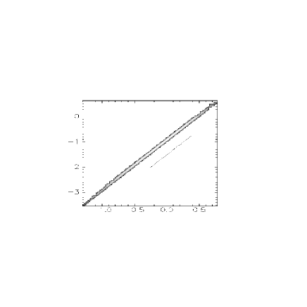
Figure 1: Log-log scatter plot of the magnetic pressure versus density for a simulation with $\theta=\pi/2$, $\tilde{M}_{s}=4.12$, $\tilde{M}_{a}=5.16$, $\tilde{\beta}=1.52$, ${\tilde{\frac{\delta\rho}{\rho}}}=0.623$, ${\tilde{\frac{\delta B}{B}}}=0.618$ and $\tilde{\sigma}=0.054$. The line segment has a slope equal to 2.

The simplest case corresponds to perpendicular propagation ($\theta=\pi/2$) where only fast waves can propagate. In that case, we expect magnetic pressure to be very well correlated with density, with a dependance of the form $|b|^{2}\propto\rho^{2}$, whatever the value of $M_{a}$. This prediction is confirmed by the simulations as examplified in Fig. 1, which shows the logarithm of the two-dimensional histogram $h\left[\ln(\rho),\ln(|b|^{2}/2M_{a}^{2})\right]$ of the magnetic pressure versus density for a run with $\tilde{M}_{a}=5.16$, adding points from temporal snapshots taken every $0.1$ time units from $t=100$ to $t=10^{4}$. More precisely we display in grey scale (with black (resp. white) denoting the smallest (resp. largest) value) the logarithm of the number of points (in the space-time sample) in a given interval of $|b|^{2}/2M_{a}^{2}$ and $\rho$, plotting only the points where the histogram is larger than $90\%$ of the maximum at fixed $\rho$. We also calculate an average histogram dispersion in the following way. For each density $\rho$, we define the mean of the magnetic pressure logarithm as

$$\bar{p}_{m}(\rho)=\int_{0}^{\infty}xh\left[\ln(\rho),x\right]dx/H$$ (33)

and the dispersion as

$$\bar{\sigma}(\rho)=\left(\int_{0}^{\infty}\left[x-\bar{p}_{m}(\rho)\right]^{2}h\left[\ln(\rho),x\right]dx/H\right)^{1/2}$$ (34)

where $H=\int_{0}^{\infty}h(\rho,x)dx$. An average dispersion $\tilde{\sigma}$ is evaluated by taking the mean of $\bar{\sigma}(\rho)$ for $\ln(\rho)$ varying by $10\%$ about its central value.

,

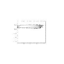
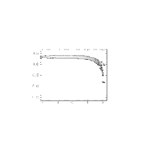
Figure 2: Log-log scatter plot of the magnetic pressure versus density for two simulations with $\cos\theta=0.1$. The parameters of the left panel, corresponding to a case with forcing on all three velocity components are $\tilde{M}_{s}=6.63$, $\tilde{M}_{a}=0.478$, $\tilde{\beta}=0.00685$, ${\tilde{\frac{\delta\rho}{\rho}}}=2.69$, ${\tilde{\frac{\delta B}{B}}}=0.323$ and $\tilde{\sigma}=0.18$. For the right panel, where the forcing is applied on the $v$ velocity components only, $\tilde{M}_{s}=7.27$, $\tilde{M}_{a}=0.527$, $\tilde{\beta}=0.00728$, ${\tilde{\frac{\delta\rho}{\rho}}}=3.55$, ${\tilde{\frac{\delta B}{B}}}=0.324$ and $\tilde{\sigma}=0.059$.

Figure 3: Top: Snapshot of $\log_{10}\rho$ (solid) and $\log_{10}|b|^{2}$ (dotted) for the run of Fig. 2a. Bottom: Density PDF for the run of Fig. 2a in log-log coordinates. The dashed line shows a fit of the curve with a parabola corresponding, in these coordinates, to a lognormal distribution.

As the angle $\theta$ is decreased from $\pi/2$, the behavior is very sensitive to $M_{a}$. When $M_{a}\ll 1$ the field lines are still almost unperturbed but the density fluctuations are very different from the case $\theta=\pi/2$ because for small $\beta$ the latter are mostly created by slow waves. In that case again we expect the magnetic pressure to exhibit little scatter, as the field is only slightly perturbed, and to be roughly anti-correlated with density, as the total pressure remains roughly constant. This is indeed the case, as seen in Fig. 2a. where the distribution of $|b|^{2}/2M_{a}^{2}$ and $\rho$ has a small scatter. In addition, a clear anticorrelation is observed at high density when no forcing is applied on the $x$-component of the velocity (Fig. 2b). In the case of purely perpendicular propagation the density structures are those typically observed in neutral turbulence with a polytropic index $\gamma=2$, i.e. rather flat-topped structures (plateaux) separated by shocks that keep interacting, with a preeminence of low density regions (Passot & Vázquez-Semadeni (1998)). In contrast, for nearly perpendicular propagation and $M_{a}\ll 1$, the density structures are composed of large peaks that oscillate while avoiding collision (Fig. 3a). The probability density function (PDF) of the density shown in Fig. 3b shows an extended tail at large density with a significant excess at small density. Since the field strength is roughly constant and independent of $\rho$, the magnetic pressure term in eq. (2) acts like an random acceleration whose strength increases as $\rho$ decreases since $|b|^{2}$ is roughly constant at small density (see Fig. 2a). Whereas the density field of an isothermal gas stirred by a random acceleration has a lognormal distribution, when the acceleration depends on the density, the PDF ceases to be lognormal (Passot & Vázquez-Semadeni (1998)). The lift up of the left tail seen in Fig. 3b is thus expected in the present case.

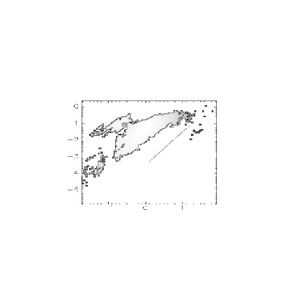
Figure 4: Log-log scatter plot of the magnetic pressure versus density for a simulation with forcing on the three velocity components, $\cos\theta=0.1$, $\tilde{M}_{s}=5.73$, $\tilde{M}_{a}=7.29$, $\tilde{\beta}=1.53$, ${\tilde{\frac{\delta\rho}{\rho}}}=1.32$, ${\tilde{\frac{\delta B}{B}}}=2.17$ and $\tilde{\sigma}=0.61$. The line segment has a slope equal to 2.

Figure 5: Top: Snapshot of $\log_{10}\rho$ (solid) and $\log_{10}|b|^{2}$ (dotted) for the run of Fig. 4. Bottom: Density PDF for the run of Fig. 4 in log-log coordinates. The dashed shows a lognormal fit.

When the angle $\theta$ is still slightly smaller than $\pi/2$ but with $M_{a}\gg 1$, the magnetic field lines undergo large fluctuations and both slow and fast waves contribute to the production of density fluctuations. As seen in Fig. 4, and Fig. 5a, magnetic pressure and density are now positively correlated (magnetic pressure roughly follows a polytropic law with $\gamma=2$, corresponding to the fast mode), but the dispersion is larger than in the case of a small Alfvénic Mach number, indicative of the additional contribution of the slow mode. As a result, the stirring due to magnetic pressure is statistically non-correlated with the density and the density PDF is expected to be much closer to a lognormal as seen in Fig. 5.

,

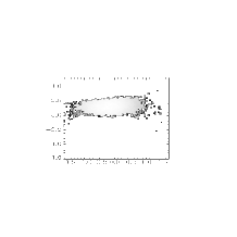
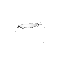
Figure 6: Log-log scatter plot of the magnetic pressure versus density for two simulations with forcing on the three velocity components and $\cos\theta=0.7$. The parameters of the left panel are $\tilde{M}_{s}=2.90$, $\tilde{M}_{a}=0.521$, $\tilde{\beta}=0.00375$, ${\tilde{\frac{\delta\rho}{\rho}}}=1.20$, ${\tilde{\frac{\delta B}{B}}}=0.473$ and $\tilde{\sigma}=0.32$. For the right panel $\tilde{M}_{s}=6.59$, $\tilde{M}_{a}=2.48$, $\tilde{\beta}=0.141$, ${\tilde{\frac{\delta\rho}{\rho}}}=1.43$, ${\tilde{\frac{\delta B}{B}}}=9.62$ and $\tilde{\sigma}=0.49$.

When the angle $\theta$ is intermediate between parallel and almost perpendicular propagation, the distinction between the small and the large Alfvénic Mach number cases is not as clear. As shown in Figs. 6a-b for runs with an angle $\theta\approx\pi/4$ and for $\tilde{M}_{a}=0.521$ and $\tilde{M}_{a}=2.48$ respectively, there is a larger scatter of the points for small to intermediate values of the density at large Alfvénic Mach number. In this case a positive correlation between magnetic pressure and density is noticeable at large density (Fig. 6b).

,

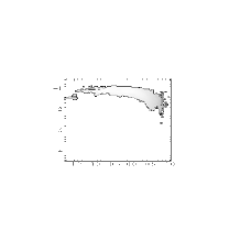
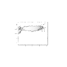
Figure 7: Log-log scatter plot of the magnetic pressure versus density for two simulations with $\theta=0$. The parameters of the left panel, where the forcing only affects the perpendicular velocity components, are $\tilde{M}_{s}=2.72$, $\tilde{M}_{a}=1.76$, $\tilde{\beta}=0.440$, ${\tilde{\frac{\delta\rho}{\rho}}}=1.04$, ${\tilde{\frac{\delta B}{B}}}=4.73$ and $\tilde{\sigma}=0.21$. For the right panel, where the forcing is applied on the three velocity components, $\tilde{M}_{s}=5.10$, $\tilde{M}_{a}=2.36$, $\tilde{\beta}=0.218$, ${\tilde{\frac{\delta\rho}{\rho}}}=1.73$, ${\tilde{\frac{\delta B}{B}}}=7.91$ and $\tilde{\sigma}=0.57$.

For parallel propagation with perpendicular forcing, the behavior is again strongly dependent on the Alfvénic Mach number. When $M_{a}\gg 1$, the magnetic field is strongly distorted. The forcing excites slow modes which develop into shocks, inside which large density clumps form. These clumps, located at local minima of the magnetic field intensity, are separated by regions of large magnetic pressure (Fig. 8a). As a result, they can hardly approach each other but rather oscillate about their mean position, at a frequency close to that of the fast wave of the local total magnetic field. The signature of the slow wave dominance is the rather small scatter and the anti-correlation between magnetic pressure and density in compressed regions, as seen in Fig. 7a corresponding to a case with $\tilde{M}_{a}=1.76$. In a way similar to the case of small $M_{a}$ and almost perpendicular propagation, the density PDF shown in Fig. 8, displays an excess at small density.

Figure 8: Top: Snapshot of $\log_{10}\rho$ (solid) and $\log_{10}|b|^{2}$ (dotted) for the run of Fig. 7a. Bottom: Density PDF for the run of Fig. 7a in log-log coordinates. The dashed shows a lognormal fit.

At small values of $M_{a}$, the magnetic field undergoes mild variations. The perpendicular forcing preferentially excites fast waves but the slow waves that form by nonlinear interactions are the most effective at producing density fluctuations since, the field being almost straight, only thermal pressure acts against compression at dominant order (see below for the effect of Alfvén wave pressure). In contrast with the case of large $M_{a}$, a larger scatter is observed on the magnetic pressure vs. density diagram, as seen on Fig. 9. As seen on Fig. 10a, the correlation between density and magnetic field intensity is lost and the density PDF is closer to a lognormal (Fig. 10b).

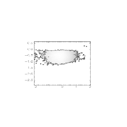
Figure 9: Log-log scatter plot of the magnetic pressure versus density for a simulation with $\theta=0$ and forcing on the perpendicular velocity components. The parameters are $\tilde{M}_{s}=5.34$, $\tilde{M}_{a}=0.172$, $\tilde{\beta}=0.00108$, ${\tilde{\frac{\delta\rho}{\rho}}}=1.37$, ${\tilde{\frac{\delta B}{B}}}=0.168$ and $\tilde{\sigma}=0.56$.

Figure 10: Top: Snapshot of $\log_{10}\rho$ (solid) and $\log_{10}|b|^{2}$ (dotted) for the run of Fig. 9. Bottom: Density PDF for the run of Fig. 9 in log-log coordinates. The dashed shows a lognormal fit.

The behavior of the Alfvén wave pressure can also be tested numerically. We have chosen to take $\beta=0$ (by turning off the thermal pressure term), in order to make its effect more visible. In a run with parallel propagation, the forcing is now applied on modes 49-51 for the perpendicular velocity components and on modes 1-5 for the longitudinal component. Three different simulations have been performed, with $\tilde{M}_{a}=0.073,0.795$ and $2.09$. As visible on Figs. 11-13, while the magnetic pressure roughly behaves as $\rho^{1/2}$ for $M_{a}=0.4$, a clear tendency to approach a polytropic behavior with $\gamma=2$ is observed when $M_{a}$ increases.

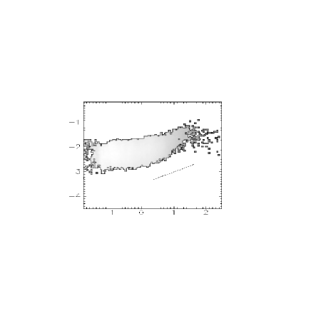
Figure 11: Log-log scatter plot of the magnetic pressure versus density for a simulation with $\theta=0$ and $\beta=0$ The parameters are $\tilde{M}_{a}=0.073$, ${\tilde{\frac{\delta\rho}{\rho}}}=3.94$, ${\tilde{\frac{\delta B}{B}}}=0.0564$ and $\tilde{\sigma}=0.60$. The line segment has a slope 0.5

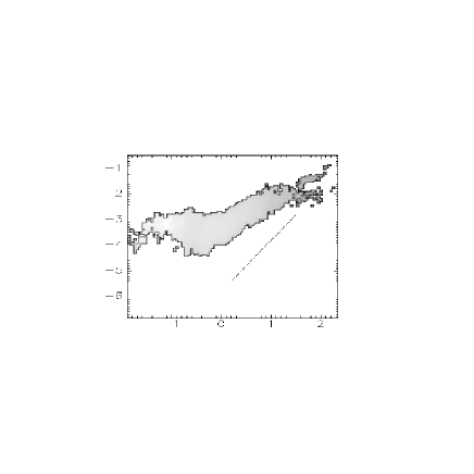
Figure 12: Log-log scatter plot of the magnetic pressure versus density for a simulation with $\theta=0$ and $\beta=0$ The parameters are $\tilde{M}_{a}=0.795$, ${\tilde{\frac{\delta\rho}{\rho}}}=4.18$, ${\tilde{\frac{\delta B}{B}}}=0.311$ and $\tilde{\sigma}=0.63$. The line segment has a slope 2.

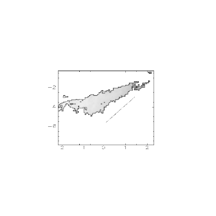
Figure 13: Log-log scatter plot of the magnetic pressure versus density for a simulation with $\theta=0$ and $\beta=0$ The parameters are $\tilde{M}_{a}=2.09$, ${\tilde{\frac{\delta\rho}{\rho}}}=3.503$, ${\tilde{\frac{\delta B}{B}}}=1.01$ and $\tilde{\sigma}=0.76$. The line segment has a slope 2.

5 Conclusions

5.1 Summary and discussion

In this paper we have investigated the dependence of the magnetic pressure, $B^{2}$ (and therefore, of the magnetic field strength) on density in fully turbulent flows, parameterized by the Alfvénic Mach number $M_{a}$ (which provides a more direct measure of the amount of field distorsion than $\beta$) of the flow and the angle between the mean field direction and the direction of wave propagation. To do this, we first employed the simple-wave formalism to obtain insight by deriving relations between the fluctuations of the magnetic and velocity fields on one hand, and the density fluctuations on the other. We then presented numerical experiments confirming the expectations from the analysis, and extended the results.

From the simple-wave analysis, we concluded that the production of density fluctuations is dominated by the slow mode at low $M_{a}$, while at large $M_{a}$ both modes contribute. This result is in disagreement with the assumption of Lithwick & Goldreich (2001) that the fast mode can be neglected in accounting for the spectrum of density fluctuations because it decouples from the Alfvén and slow modes due to its larger phase speed. Moreover, except for the case of small field fluctuations with simultaneously moderate density fluctuations and parallel field component, the magnetic pressure behaves as

$$P_{\rm mag}\simeq c_{1}-c_{2}\rho$$ (35)

for the slow mode, and as

$$P_{\rm mag}\simeq\rho^{2}$$ (36)

for the fast mode. This different scaling of the magnetic pressure with density for the two modes is at the basis of the decorrelation observed, as in general a given value of the density can be arrived at by a different kind of wave, and therefore have a different associated value of the magnetic pressure. More generally, we can say that the particular value of the magnetic pressure of a fluid parcel will not be uniquely determined by its density, but instead, that it will depend on the detailed history of how the density fluctuation was arrived at. This also implies that turbulent pressure cannot be simply modeled with a polytropic law in general, and in fact it can act as a “random” forcing instead of as a restoring force. In particular, strong density fluctuations are possible even in the presence of a large uniform magnetic field, but in general there is no relation between $\delta\rho/\rho$ and $\tilde{\beta}$.

The angle $\theta$ between the the mean field and the direction of wave propagation also plays an important role in determining the relative importance of the modes. At perpendicular propagation, the slow mode does not propagate, but at almost perpendicular propagation and low $M_{a}$ it is dominant. At intermediate angles, the distinction between the low- and high-$M_{a}$ cases is less pronounced, although at large $M_{a}$ a tighter correlation between density and magnetic field strength is observed at high densities. Also, in some cases (parallel propagation at moderate to large $M_{a}$), density peaks can even correspond to magnetic pressure minima. This is in fact reminiscent of pressure balanced structures commonly observed in the solar wind and possibly present in the ISM (see the simulations Mac Low et al 2001).

Our results have implications on the functional form of the density PDF. We found that it tends to be lognormal, due to the unsystematic action of the magnetic pressure, which allows the thermal pressure to take control, except when the slow mode dominates density fluctuation production. In this case, the strength of the random forcing-like action of the magnetic pressure becomes density-dependent, and causes a low-density excess in the PDF.

We also presented a perturbative analysis of the Alfvén-wave pressure, which recovered all the limiting polytropic cases obtained by MZ (95), with $\gamma_{e}\simeq 2$ at large $M_{a}$, $\gamma_{e}\simeq 3/2$ at moderate $M_{a}$, and $\gamma_{e}\simeq 1/2$ at low $M_{a}$, but we also mentioned a result by Passot & Gazol (in preparation) using this approach showing that the Alfvén wave pressure is in general not isotropic. As pointed out by MZ (95), the conclusion of isotropy follows from assuming a unique relation between the fluctuations of the velocity and of the magnetic field, valid for a traveling Alfvén wave. That isotropy does not hold in general is evidence that all three wave modes contribute to the velocity fluctuations, each one with a different functional form, similarly to the different scalings of magnetic pressure with density for the slow and fast modes.

5.2 Implications

Our results have a number of interesting implications on the standard picture for the support of molecular clouds by magnetic fields, and on the interpretation of observations. Observational surveys of the magnetic field strength in molecular clouds seem to indicate that the former is essentially uncorrelated from the density at low ($\lower 2.15277pt\hbox{$\;\buildrel<\over{\sim}\;$}10^{3}$ cm^-3) densities, with recorrelation seemingly appearing at higher densities (e.g., Crutcher et al. 2002). In particular, in molecular clouds non-detections of the Zeeman effect are generally more frequent than detections, and so in many cases only upper limits to the field strength are available (e.g., Crutcher et al. 1993; Bourke et al. 2001). Although it has been argued that these results are consistent with the standard theory of molecular cloud support (Shu, Adams & Lizano 1987) through consideration of statistical corrections to the random orientations of the field with respect to the line of sight (Crutcher et al. 1993; Crutcher et al. 2002), it is clear that they are also consistent with the lack of correlation between field strength and density found in the present paper and in other numerical simulations (Padoan & Nordlund 1999; Ostriker et al. 2001). This has been already pointed out by Padoan & Nordlund (1999).

The recorrelation apparently observed at higher densities (also noticeable in the 3D simulations of Ostriker et al. (2001) including self-gravity) is consistent with our cases with intermediate values of $\theta$ and large $M_{a}$, suggesting that the Alfvénic Mach number in molecular clouds is relatively large. However, it is also possible that this is an effect of self-gravity becoming important, which we have not considered here. It is also possible that even at high densities the magnetic field strength is highly variable from one core to another. More observations of the magnetic field strength in high-density molecular cloud cores, reporting both detections and non detections, are needed.