Interferometric Observations of the Nuclear Region of Arp 220 at Submillimeter Wavelengths

Abstract

We report the first submillimeter interferometric observations of an ultraluminous infrared galaxy. We observed Arp 220 in the CO J=3-2 line and 342 GHz continuum with the single baseline CSO-JCMT interferometer consisting of the Caltech Submillimeter Observatory (CSO) and the James Clerk Maxwell Telescope (JCMT). Models were fit to the measured visibilities to constrain the structure of the source. The morphologies of the CO J=3-2 line and 342 GHz continuum emission are similar to those seen in published maps at 230 and 110 GHz. We clearly detect a binary source separated by $\sim 1\arcsec$ in the east-west direction in the 342 GHz continuum. The CO J=3-2 visibility amplitudes, however, indicate a more complicated structure, with evidence for a compact binary at some velocities and rather more extended structure at others. Less than 30% of the total CO J=3-2 emission is detected by the interferometer, which implies the presence of significant quantities of extended gas. We also obtained single-dish CO J=2-1, CO J=3-2 and HCN J=4-3 spectra. The HCN J=4-3 spectrum, unlike the CO spectra, is dominated by a single redshifted peak. The HCN J=4-3/CO J=3-2, HCN J=4-3/HCN J=1-0 and CO J=3-2/2-1 line ratios are larger in the redshifted (eastern) source, which suggests that the two sources may have different physical conditions. This result might be explained by the presence of an intense starburst that has begun to deplete or disperse the densest gas in the western source, while the eastern source harbors undispersed high density gas.

1 Introduction

Ultraluminous infrared galaxies contain extraordinary nuclear starbursts and, at least in some cases, an active galactic nucleus, all hidden within a dense shroud of gas and dust. Understanding the mechanisms which produce and power these luminous galaxies has taken on added urgency with the discovery of their young counterparts at cosmological distances (Ivison et al., 2000). The nearest and prototype ultraluminous infrared galaxy, Arp 220, is located at a distance of 73 Mpc ($H_{o}=75$ km s^-1) and is one of the best studied of this class of galaxies. The presence of tidal tails observed in the optical (Arp, 1966; Joseph & Wright, 1995) as well as two compact emission peaks at near-infrared (Scoville et al., 1998), millimeter (Scoville, Yun, & Bryant 1997, hereafter SYB ; Downes & Solomon 1998, hereafter D&S ; Sakamoto et al. 1999, hereafter S (99)), and radio wavelengths (Becklin & Wynn-Williams, 1987; Norris, 1988; Sopp & Alexander, 1991) suggests that Arp 220 is a recent merger. Given the observed correlation between high infrared luminosity and disturbed optical morphologies indicative of galaxy interactions (Mirabel & Sanders, 1989), this merger is likely responsible for the extremely high infrared luminosity of Arp 220 [$1.4\times 10^{12}$ L_☉, Soifer et al. (1987)]. There has been much debate as to whether the high infrared luminosity is due to a starburst or an active nucleus or a combination of the two, both for Arp 220 in particular and for ultraluminous infrared galaxies in general (Genzel et al., 1998; SYB, ; Lutz et al., 1996). Recent radio studies of Arp 220 provide support for the starburst hypothesis: the 18 cm flux seen in VLBI observations is thought to be emitted by luminous radio supernovae (Smith et al., 1998) and the effects of these supernovae winds are seen in X-rays (Heckman et al., 1996). Near-infrared (Emerson et al., 1984; Rieke et al., 1985; Sturm et al., 1996; Lutz et al., 1996) and earlier radio observations (Condon et al., 1991; Sopp & Alexander, 1991; Baan & Haschick, 1995) further support the starburst scenario.

Besides its extremely high infrared luminosity, Arp 220 also contains large amounts of dust and molecular gas ($\sim 9\times 10^{9}M_{\sun}$ SYB ); large gas masses of $4-40\times 10^{9}M_{\sun}$ are typical for ultraluminous infrared galaxies (Sanders et al., 1991). The extinction at optical wavelengths is estimated to be at least $A_{V}\sim 50$ and possibly as high as $A_{V}\sim 1000$ (Sturm et al., 1996; D&S, ); even at near-infrared wavelengths (2.2$\mu$m), dust lanes obscure the possible nuclei (Scoville et al., 1998) These high extinctions mean that radio observations are needed to probe the deep interior regions. D&S have mapped Arp 220 in CO J=2-1 and 1.3 mm continuum; besides detecting two emission peaks, they also see an extended disk (with full-width half-maximum extent of $2\arcsec\times 1.6\arcsec$). They interpret the emission peaks as the nuclei of the merging galaxies embedded in a more extended disk of molecular gas. S (99) refine the model further using their CO J=2-1 and continuum observations; in this model, the nuclei are each embedded in their own gas disk which is counter-rotating in the larger common disk. An alternative interpretation of the emission peaks as being due to crowding in the orbits of molecular gas and stars is given by Eckart & Downes (2001).

This paper presents the very first interferometric submillimeter observations of Arp 220 in the CO J=3-2 line and 0.88 mm continuum. In fact, it is the first paper to present data from submillimeter interferometry of any extragalactic source. We also present single dish observations of Arp 220 of HCN J=4-3, a high density tracer. Furthermore, to determine the total CO flux of Arp 220, which could be partly resolved out by the interferometer, complementary single dish data were taken in CO J=3-2 as well as in the CO J=2-1 line. These submillimeter observations allow us to penetrate deep into the interior of the nuclei, while at the same time tracing hotter gas, which may be more closely associated with the source of the ultraluminous infrared luminosity. We describe the observations in § 2 and the data analysis in § 3. The interferometric data were obtained with the single baseline CSO-JCMT interferometer, the only currently available submillimeter interferometer with sufficient bandwidth to observe the broad emission lines of Arp 220. With data from a single baseline, mapping is not possible and so we analyze the data by making fits in the visibility plane. The data are compared to published data at lower frequencies and to single dish data in § 4 and the conclusions are presented in § 5.

2 Observations and Data Reduction

2.1 Interferometric Data

The interferometric measurements were obtained with the CSO-JCMT interferometer on Mauna Kea, Hawaii, consisting of the Caltech Submillimeter Observatory (CSO) and the James Clerk Maxwell Telescope (JCMT). Usually these two telescopes are operated independently for single dish observations, but occasionally they are linked together as a submillimeter interferometer with a single baseline of 164 m and a minimum fringe spacing of 1.1^′′ at 350 GHz (Lay et al., 1994a; Lay, 1994b; Lay, Carlstrom, & Hills, 1995, 1997). The CSO-JCMT interferometer is currently the only submillimeter interferometer with a bandwidth broad enough to accommodate the $\sim 800$ km s^-1 wide line of Arp 220.

The ¹²CO J=3-2 transition and associated continuum emission at 342.5 GHz of Arp 220 were observed on 1997 May 10 in good weather with 1.4 mm of precipitable water vapor. The coordinates of Arp 220 used were $\alpha$(2000)=15^h 34^m 57.^s19, $\delta$(2000)=23^∘ 30${}^{{}^{\prime}}$ 11$\farcs$3 (originally $\alpha$(1950)=15^h 32^m 46.^s91, $\delta$(1950)=23^∘ 40${}^{{}^{\prime}}$ 07$\farcs$9). To monitor the gain of the system, these observations were interleaved with those of the quasar 3C 345. Continuum and line observations of Arp 220 and 3C 345 were alternated in time. We also observed the quasar 3C 273 in both single dish and interferometric mode to determine the absolute flux calibration; the interferometric observations were additionally used to determine the shape of the passband. Figure 1 shows the (u, v) track of the CO J=3-2 data with a fringe spacing ranging from $1\farcs 2$ to $5\farcs 8$.

Figure 1: Track of CO J=3-2 interferometric observations in (u, v) coordinates.

Both the Arp 220 and the 3C 345 data were divided by a passband created from observations of 3C 273. Changes in the relative gain of the interferometer as a function of time were then calibrated by applying the gain curve derived from observations of the point source 3C 345 to the Arp 220 data. Each set of ten 10-second integrations was vector-averaged to produce a series of 100-second integrations with higher signal-to-noise ratios.

Figure 2: Interferometric CO J=3-2 spectra. The histogram shows the flux on a scale of 0 to 2.4 Jy. The dashes are the phase, where the upper half of each plot covers the phase from $-\pi$ to $\pi$. The velocities are relative to 339.5 GHz corresponding to a velocity of 5450 km s^-1 in the radio definition. The first spectrum on the top left was taken at -2.3 h (HA) at (u, v) coordinates (-140 k$\lambda$,90 k$\lambda$), the top right at HA=-0.8 h (-170 k$\lambda$,60 k$\lambda$), middle left at HA=2 h (-160 k$\lambda$,10 k$\lambda$), middle right at HA=3.2 h (-125 k$\lambda$,-10 k$\lambda$), bottom left at HA=4.5 h (-70 k$\lambda$,-20 k$\lambda$), bottom right at HA=5.5 h (-25 k$\lambda$,-25 k$\lambda$). The continuum - measured at slightly different (u, v) positions - was extrapolated to the above (u, v) positions (using our best fitting binary model) and the expected continuum emissions of 0.16, 0.31 0.28, 0.15, 0.2 and 0.35 Jy have been subtracted from the respective line data.

The spectra displayed in Figure 2 were further averaged to 1000 seconds. (The sixth spectrum only contains 500 seconds of data.) Since the average phase might drift over time scales longer than 100 seconds due to instrumental or atmospheric phase shifts, the average phase over the whole frequency range of each 100-second sample was measured and then subtracted from the phases in each of the individual velocity channels. The resultant line data were then averaged by deriving the arithmetic means of the sine and cosine components in each individual channel.

By comparing single dish measurements of Mars with those of 3C 273, we obtained a flux of $12\pm 0.5$ Jy for 3C 273, which agrees very well with the value of 12.2 Jy measured at 850 $\mu$m with SCUBA around the same time (Robson, Stevens, & Jenness, 2001). We used the 3C 345 measurements immediately before and after the 3C 273 data and obtained a 3C 345 flux of 0.90 Jy averaged over the emission at 342.5 and 339.5 GHz. After averaging and gain calibrating the Arp 220 and 3C 345 data in exactly the same way, the scalar average of the 3C 345 data was determined and from it the conversion factor from K to Jy. This conversion may vary between the continuum and CO data and with velocity bin because the gain calibration can vary with frequency range. We derived conversion factors ranging from $48$ Jy K^-1 to $59$ Jy K^-1. The overall uncertainty in the calibration due to gain variations and uncertainties in the planet flux is estimated to be 20% (Lay, 1994b).

Since the continuum data were measured at different (u, v) positions than the line data, we extrapolated the continuum data using the binary model discussed in §3.3 and subtracted 0.16, 0.31, 0.28, 0.15, 0.2 and 0.45 Jy from the six CO measurements (with increasing hour angle), respectively. All velocities quoted use the radio definition ($v_{rad}=c(\nu_{rest}-\nu_{obs})/\nu_{rest}$) with respect to the local standard of rest (lsr).

2.2 Single-Dish Data

On 1997 July 17 and 18 we used the JCMT to observe emission lines from ¹²CO J=3-2, ¹²CO J=2-1, and HCN J=4-3 under good weather conditions. The observations were made with the facility 230 GHz (A2) and 350 GHz (B3) receivers, which had system temperatures of 270-360 K and 400-600 K, respectively, in the center of the spectral window. The spectra were obtained with a chopping secondary mirror using a switch cycle of 1 Hz and a beam throw of 60^′′ in azimuth. We configured the DAS to give a spectral resolution of 1.25 MHz with a bandwidth of 1.86 GHz for B3 and 0.95 GHz for A2. The relative errors in pointing were small, $\sim 2^{\prime\prime}$ rms for A2 and $\sim 3^{\prime\prime}$ rms for B3, with significant systematic errors in the pointing apparent when observing at elevations greater than 80^o. Spectra obtained at such high elevations were not used in the subsequent analysis.

Our data were flux calibrated through observations of Mars and Uranus. We found significant differences between our derived aperture efficiencies and the typical aperture efficiencies for the JCMT. We derive aperture efficiencies of 0.48 at 230 GHz, 0.42 at 265 GHz, and 0.43 at 345 GHz, compared to the standard telescope values of 0.69 at 230 GHz and 0.58 at 345 GHz. We adopt 20% as the error in the absolute calibration of our single dish observations. We present all our single dish data on the T${}^{*}_{A}$ temperature scale, which is most appropriate for the compact nuclear emission seen in Arp 220 (SYB, ; S, 99; D&S, ).

Figure 3: CO J=2-1 and CO J=3-2 spectra with a resolution of 22$\arcsec$. For CO J=2-1 the integrated intensity is 53 K km s^-1 or 1730 Jy km s^-1. For CO J=3-2 the integrated intensity over the same 22$\arcsec$ beam is 45 K km s^-1 or 3700 Jy km s^-1.

We used the package SPECX (Padman, 1993) to reduce the spectra and used first-order baselines in all cases. The CO J=2-1 spectrum is shown in Figure 3. We derive an integrated intensity of 53 K km s^-1, which for a conversion factor of 32.6 Jy K^-1(T${}_{A}^{*}$) corresponds to a flux of 1730 Jy km s^-1. This value is significantly larger than the flux determined by Radford, Solomon, & Downes (1991) in a 12^′′ beam (1040 Jy km s^-1). The interferometric maps of SYB and D&S show very compact CO J=2-1 emission with a total extent of roughly $4\times 4^{\prime\prime}$. The larger flux detected in the 21^′′ beam of the JCMT suggests that there may also be extended CO J=2-1 emission with roughly half the total intensity seen in the nuclear region. However, we also obtained CO J=2-1 spectra at positions offset 11^′′ (half a beam width) from the central position; the flux in those offset spectra is roughly half that in the center, consistent with quite compact emission in the central region.

Figure 4: Map of CO J=3-2 emission with a resolution of 15$\arcsec$. The integrated intensity in the central spectrum is 84 K km s^-1 or 2980 Jy km s^-1

A small map of the CO J=3-2 emission is shown in Figure 4. For the central position we derive an integrated intensity of 84 K km s^-1, which for a conversion factor of 35.5 Jy K^-1 (T${}_{A}^{*}$) corresponds to a flux of 2980 Jy km s^-1. When we convolve this map to simulate the 21^′′ beam of the CO J=2-1 spectrum, we derive an integrated intensity of 45 K km s^-1 or 3700 Jy km s^-1. This integrated intensity is somewhat larger than the value of 32 K km s^-1 obtained in a similar beam by Gerin & Phillips (1998), but agrees well with the measurement of Mauersberger et al. (1999). Combining the convolved spectrum with the CO J=2-1 data gives a CO J=3-2/J=2-1 ratio of $0.85\pm 0.24$, where the uncertainty includes the estimated 20% calibration uncertainty in each line.

Figure 5: HCN J=4-3 with a resolution of 15$\arcsec$. The integrated intensity is 7.1 K km s^-1 or 260 Jy km s^-1.

The HCN spectrum is shown in Figure 5, with an integrated intensity of 7.1 K km s^-1 (260 Jy km s^-1) for the HCN J=4-3 transition. We can combine the HCN and CO data obtained with similar beams to obtain an HCN J=4-3/CO J=3-2 line ratio of $0.085\pm 0.024$. This line ratio is quite similar to the value of 0.12 obtained by Solomon, Downes, & Radford (1992) for the J=1-0 transitions in 23-28^′′ beams.

3 Analysis of Single Baseline Interferometric Data

The CSO-JCMT interferometer was used to measure the cross-correlated amplitude and phase of Arp 220 as a function of observing frequency and as a function of (u, v) position (Figure 1), which is related to the projected baseline. With a fixed single baseline interferometer, we cannot obtain sufficient coverage of the (u, v)plane to produce an image of the source on the sky. Nevertheless, the (u, v) data themselves contain a lot of information, which can be extracted by comparing simple models to the data (such as a single extended disk, two point sources, etc.). We analyzed the amplitude and phase data separately following the guidelines in Lay (1994b). The method of fitting models to the visibility phases is explained in § 3.1, that of fitting models to the visibility amplitudes in § 3.2 and the best model fits to our continuum and CO J=3-2 spectral line data are presented in § 3.3. Readers who are interested primarily in the results of our analysis may wish to skip directly to § 3.3.

3.1 Fitting Models to Visibility Phase

The interferometer measures the difference in path lengths from the source to the two antennas in terms of phase. When corrected for geometric and instrumental effects, this phase contains information about the source’s position in the sky. Unfortunately, the CSO-JCMT interferometer is not stable enough to determine accurately an absolute position of a source from its phase. However, with our spectral line data, it is possible to use the redshifted emission of Arp 220 as a phase reference and to measure the phase of the blueshifted emission relative to the redshifted emission. Fitting models to this phase difference as a function of (u, v) position can determine the position offset on the sky of the blueshifted emission relative to the redshifted emission. As an example, for a pure east-west baseline, a position offset in right ascension (RA) will result in a phase change proportional to the cosine of the hour angle of Arp 220, whereas an offset in declination introduces a phase change proportional to $\sin({\rm RA})\sin(\delta)$, where $\delta$ is the declination of Arp 220. More accurately, $\Delta\phi=2\pi(-u\Delta{\rm RA}-v\Delta\delta)$, where $u$ and $v$ are the (u, v) coordinates of the phase reference source, which depends on all three components of the baseline as well as the declination and hour angle of the phase reference source (Thompson, Moran, & Swenson, 2001).

3.2 Fitting Models to Visibility Amplitudes

The visibility amplitude changes as a function of time depending on the structure of the source and the length and direction of the projected baseline. The visibility of a point source, i.e. a quasar, will be constant after correction for instrumental and atmospheric effects. Therefore the visibilities of a point source, here 3C 345, are used to calibrate out any instrumental or atmospheric changes. An extended source might be partially resolved out around transit, when the projected baseline is the largest, in which case its visibility amplitude would decrease. The visibility amplitude of two point sources will be a minimum whenever their separation is a multiple of half the fringe spacing. From these very simple consideration, it is already clear from Figure 6 that our data are neither consistent with the visibility expected from a single point source nor are the data in panels (a), (d) and (e) consistent with that from a single extended source.

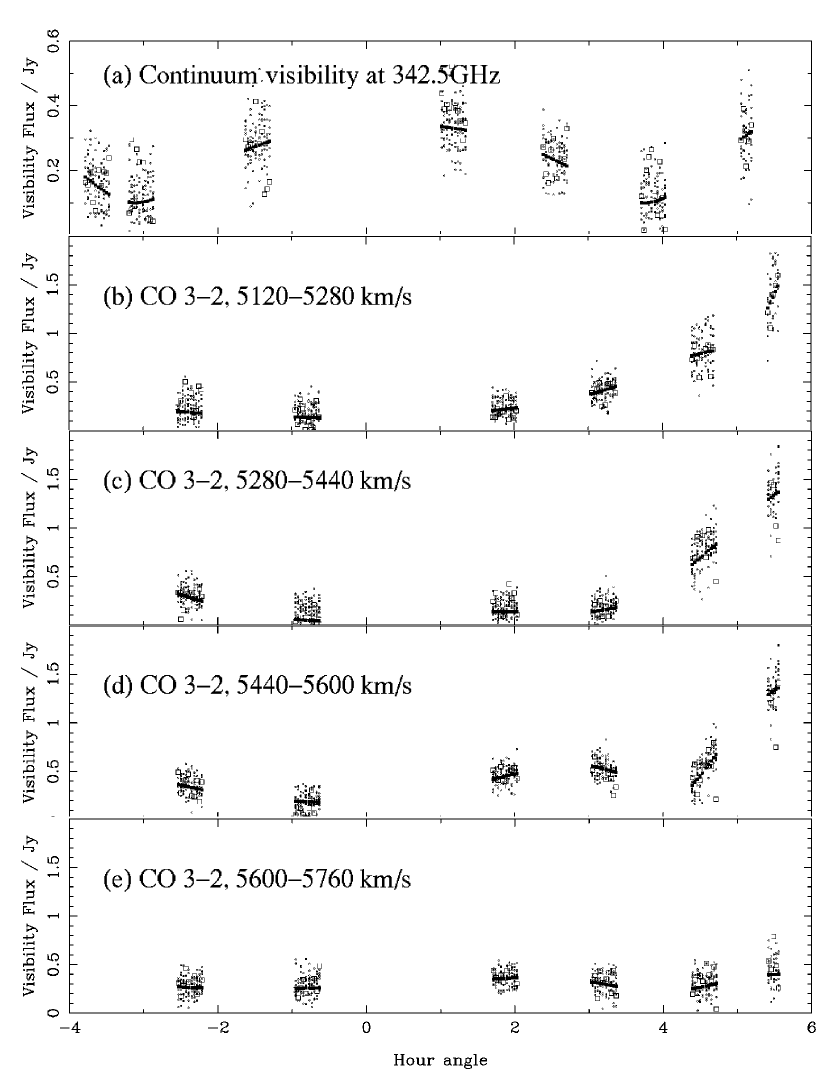
Figure 6: Visibilities and model fits to the Arp 220 data. The data are represented by squares, the model is the thick line and the dots are simulated data given the model and the measured noise. (a) Continuum data at 352.5 GHz. (For clarity the y-axis of the continuum data only runs from 0 to 0.6 Jy in contrast to 0 to 2 Jy in all other panels of the line data.) The model represents the visibility of a binary with two point-like sources with fluxes of 0.25 Jy and 0.15 Jy, and separated by $1\farcs 0$ at a position angle east of north (P.A.) of 80^o. (b) CO J=3-2 visibilities (after continuum subtraction) integrated over 5120 to 5280 km s^-1 (radio definition) and the binary model fit to the data. (Source 1: 3.2 Jy, $2\farcs 4\times 2\farcs 4$; Source 2: 0.83 Jy, $1\arcsec\times 1\arcsec$; Separation: $2\farcs 8$ at P.A. 30^o). (c) CO J=3-2 visibilities integrated over 5280 to 5440 km s^-1 and binary model fit to the data. (Source 1: 0.65 Jy, $0\farcs 9\times 0\farcs 9$; Source 2: 1.0 Jy, $0\farcs 95\times 0\farcs 95$; Separation: $1\farcs 0$ at P.A. 52^o). (d) CO J=3-2 visibilities integrated over 5440 to 5600 km s^-1 and binary model fit to the data. (Source 1: 0.55 Jy, $0\farcs 84\times 0\farcs 84$; Source 2: 0.92 Jy, $1\farcs 0\times 1\farcs 0$; Separation: $1\farcs 45$ at P.A. 115^o). (e) CO J=3-2 visibilities integrated over 5600 to 5720 km s^-1 and binary model fit to the data. (Source 1: 0.3 Jy, point-like; Source 2: 0.1 Jy, $0\farcs 6\times 0\farcs 6$; Separation: $1\farcs 7$ at P.A. 130^o).

Therefore we attempted to fit the Arp 220 data primarily with models consisting of two sources. Each source is assumed to have a Gaussian brightness distribution of an elliptical shape; this approach results in a model with 10 parameters (the separation of the two sources and the position angle of this separation; the flux, minor axis, major axis, and position angle of each source). It is possible that models with even more sources would fit the data even better. However, with measurements of the visibility amplitude at only 6 or 7 different (u, v) positions, we do not have enough data to constrain models with many more free parameters.

We used the Maximum Likelihood method to determine which source model fit the data best. We first calculated the expected visibility amplitude for each model. Since the noise of the data is known, the probability of each data point given the model can be calculated. In the case of high signal to noise, the probability is described by a Gaussian distribution. However, in our case, the noise is comparable to the signal and therefore the Rice distribution describes our data better (Thompson et al., 2001). The product of the probability of each of the data points given the model gives the likelihood of the model. The model with the greatest product of probabilities is the most likely.

For the continuum data we then calculated the Bayesian error of each of the ten parameters for the most likely model. First, the probabilities for each model were normalized by dividing them by the maximum probability. Then the probabilities of all models with the parameter $a$ having a given value $a_{1}$ were summed. (This sum is the marginal probability of $a_{1}$, which is independent of the other nine parameters.) This process was repeated for all the different values $a_{2}$, $a_{3}$ etc. of $a$. (If we had a continuous rather than a discrete set of values for $a$, this process would be equivalent to integrating the probability $p(a,b,c,...,j)$ of the ten dimensional parameter space over all parameters but $a$ to give the one dimensional marginal probability of $a$, $p_{mar}(a)=\int\!\!\dots\int\!\!\int\!p(a,b,c,\dots,j)\,db\,dc\dots dj$.) Usually, but not necessarily, the value $a_{max}$ with the highest marginal probability is also the value found for the most likely model.

In a small region around $a_{max}$, the probability distribution can be approximated by a Gaussian. We defined the one sigma Bayesian error of $a_{max}$ as the distance between $a_{max}$ and $a_{\sigma}$, where $a_{\sigma}$ is the location where the marginal probability drops to $\exp(-1/2)p_{mar}(a_{max})$. (More precisely, $a_{\sigma}$ should define the boundaries within which 68% of the marginal probability lies. In the case where the marginal probability can be approximated by a Gaussian, $p_{mar}(a_{\sigma})$ will have the value $\exp(-1/2)p_{mar}(a_{max})$. Since in our case the marginal probability distribution of the continuum data appears Gaussian, we used the latter method to determine the error.) The error on each parameter gives an indication of how well the measured data determine each parameter in a given model, but the error contains no information about the validity of the model.

For the line data the Bayesian error could not be calculated, because the marginal probability is not Gaussian, as there are large secondary maxima of the probability. We have therefore taken a different approach: after finding the most likely model, we fixed all parameters but one and defined the 1$\sigma$ error as the distance where the probability falls to $\exp(-1/2)p(a_{max})$. The difference to the continuum method is that we do not integrate over all other parameters, i.e. we are assuming that all other parameters are accurately known. The advantage of this method is that it ignores most secondary maxima, as we are only taking a one-dimensional cut in the 11-dimensional probability surface. Since we are not taking account of all other planes, the errors are much smaller and do not reflect the error due to the existence of secondary maxima. (It might help to picture a two-dimensional probability distribution as a landscape with mountains, where the two dimensional plane represents the two parameters and the height the probability. The case of the continuum data can be imagined as one very high mountain in a landscape of low hills; the line data would correspond to a complicated mountain range with many nearly equally high mountains.)

From the maximum likelihood method, we can only determine which of the models we tried is the most likely. It is, however, possible that an entirely different model we have not considered fits the data much better. For this reason it is very helpful to have maps of the source at other wavelengths (e.g. around 230 GHz), which show the morphology of the source.

3.3 Results of Model Fitting to Continuum and CO J=3-2 Data

The 342.5 GHz continuum measurements of Arp 220 were fit using both single and binary source models. A single source model did not fit the data well. Figure 6a shows the visibility data at 342.5 GHz and the best binary fit to the data. The parameters of the best binary fit are listed in Table 1, which also gives a comparison to published results from continuum data at other wavelengths. Note in particular that, while the continuum data can constrain the strength and separation of the two sources, the models cannot tell us whether the eastern or the western source is the stronger one. This limitation is due to the lack of absolute phase information as discussed in § 3.1.

Table 1: Continuum Data

	These data	S (99)	D&S	Scoville	Baan & Haschick
	342.5 GHz	230 GHz	230 GHz	2.2$\mu$m	4.83 GHz
Morphology	binary	binary	binary	three sources	binary
Total Flux (mJy)	400$\pm$40	208	175	$\cdots$	214
Separation (arcsec)	$1.0\pm 0.1$	0.9	0.8	1.13 (NE-W)	0.98
				1.05 (SE-W)
Position	$80\pm 12$	100	100	86 (NE-W)	98
Angle (deg)				108 (SE-W)
Eastern Source:
Flux mJy	150$\pm$10	66	30	$\cdots$	88
Size (arcsec2)	$<0.6^{2}$	$<0.2^{2}$	$0.6\times 0.6$	$0.34\times 0.26$ (NE)	$0.42\times 0.31$
				$0.26\times 0.23$ (SE)
Western Source:
Flux (mJy)	250$\pm$40	142	90	$\cdots$	112
Size (arcsec2)	$<0.6^{2}$	$0.32\times 0.19$	$0.3\times 0.3$	$0.49\times 0.22$	$0.30\times 0.21$
Disk
Flux (mJy)	0	0	55	$\cdots$	14
Size (arcsec2)	$\cdots$	$\cdots$	$\cdots$	$\cdots$	$\cdots$
Flux cal. error	20%	20%	20%	$\cdots$	$\cdots$

Note. — Parameters of the binary model that fits the 342.5 GHz continuum data best. The errors quoted are the 3$\sigma$ Bayesian error of the model fitting (see § 3.2). The fluxes have an additional 20% calibration error. For comparison measurements at millimeter (S, 99; D&S, ), near-infrared (Scoville et al., 1998), and radio wavelengths (Baan & Haschick, 1995) are also listed. The radio fluxes quoted are from the naturally weighted 4.83 GHz continuum maps.

Figure 7: Measurement of source separation using the phase difference between the blueshifted (5290-5440 km s^-1) and redshifted (5550-5810 km s^-1) emission of Arp 220. The top graph shows the phase of the redshifted emission, the bottom graph shows the phase of the blueshifted emission. In both cases, a line fitting the phase of the redshifted emission has been subtracted; the scatter in the red phase therefore represents the noise in the data. The model fit is represented by the thick line and suggests an offset of ($0.\arcsec 08$,$-0.\arcsec 12$) for the redshifted emission from an arbitrary phase reference and ($-1.\arcsec 28$, $0.\arcsec 18$) for the blueshifted emission.

To determine the relative location of the two CO emission peaks, we divided the CO J=3-2 spectra into two velocity bins. We chose a velocity range (radio definition) from 5290 - 5440 km s^-1 for the blue component, and 5550 - 5810 km s^-1 for the red component. We fit a smooth “gain” curve to the phase of the red emission versus time and then subtracted this curve from both the red and blue phase. The results of this phase referencing are shown in Figure 7. We then fit models to both the red and the blue phase data using the method described in § 3.1, with the result that the averaged blue emission originates from a location offset by $-1.\arcsec 36\pm 0.\arcsec 14$ in right ascension and $0.\arcsec 30\pm 0.\arcsec 14$ in declination from the averaged red emission. In the simple case where all of the redshifted emission is emitted from one point-like component and all the blueshifted emission from another, this result gives the separation of the two components. However, the analysis of the CO J=3-2 amplitude data described below shows that this model of two point sources may be an over-simplification. Therefore, the result from the phase data may only give a rough estimate of the separation of the two locations producing most of the CO J=3-2 emission. From the phase data, it is certain, however, that the redshifted and blueshifted CO J=3-2 emission originate from different locations in Arp 220.

Published lower frequency maps show CO J=2-1 and J=1-0 emission with a complex morphology (D&S ; S (99)), which may be difficult to model with simple single or binary source models. To simplify the morphology to some extent, we divided the CO data in four velocity bins of 5120 - 5280 km s^-1, 5280 - 5440 km s^-1, 5440 - 5600 km s^-1 and 5600 - 5760 km s^-1, each of which corresponds to four velocity channels in Figure 20 from D&S . But even in these narrower velocities bins, the CO J=2-1 emission is complex. In addition, our single (u, v) track cannot sample the more extended emission adequately, nor does it have much north-south resolution.

The visibility amplitude plots themselves show some clear signatures of the source structure. Figure 6b-d all show an increase in amplitude around an hour angle of 5 h, which indicates extended emission in the east-west direction that was resolved out at longer baselines. In contrast, the highly redshifted component of the line in Figure 6e does not show a rise in amplitude as Arp 220 sets, which means that there is no extended (arcsecond scale) east-west component at these velocities. The continuum data in Figure 6a also do not show a large increase in amplitude at this hour angle.

Table 2: Best Fitting Models to CO 3-2 Interferometer Data

CO J=3-2	5120-5280	5280-5440	5440-5600	5600-5760
Vel. Bin	km s-1	km s-1	km s-1	km s-1
Separation (arcsec)	2.8$\pm$0.3	1.0$\pm$0.1	1.45$\pm$0.1	1.7$\pm$0.3
Position Angle (deg)	30$\pm$6	52$\pm$9	115$\pm$6	130$\pm$12
Eastern Source
Flux (Jy)	$\cdots$	$\cdots$	0.55$\pm$0.15	0.3$\pm$0.06
Diameter (arcsec)	$\cdots$	$\cdots$	0.84$\pm$0.12	$<$0.6
Western Source
Flux (Jy)	0.83$\pm$0.18	0.65$\pm$0.3	0.92$\pm$0.12	$\cdots$
Diameter (arcsec)	1.0$\pm$0.3	0.9$\pm$0.25	1.0$\pm$0.12	$\cdots$
Disk
Flux (Jy)	3.2$\pm$0.6	1.0$\pm$0.15	$\cdots$	0.1$\pm$0.12
Size (arcsec2)	2.4$\pm$1.2	0.95$\pm$0.12	$\cdots$	0.6$\pm$0.6
Pos. Angle (deg)	$\cdots$	$\cdots$	$\cdots$	90

Note. — Parameters of models fitting the visibilities in four different velocity ranges of CO J=3-2 emission. The data do not constrain the models well and we have chosen the model that is most consistent with the CO J=2-1 maps of D&S . The errors quoted here are the 3$\sigma$ errors of each parameter under the assumption that all other parameters are correct (see § 3.2). There are additional, mainly systematic, errors discussed in § 3.2 such that the overall error might be as large as a factor of 2.

For the line data (in contrast to the continuum data), there are many very different models which fit each set of visibility amplitudes fairly well. Of these models, we have chosen the one which seemed most consistent with the CO J=2-1 maps of D&S . The visibility data and the model fits are shown in Figure 6 and the parameters of the model are listed in Table 2. The errors in Table 2 are 3$\sigma$ errors of each parameter assuming all other parameters are accurately known (see § 3.2). In addition to those errors there are: (1) an error due to the existence of secondary maxima (i.e. a completely different combination of parameters might give a nearly equally good fit); (2) an error due to only trying binary models; (3) an error due to the uncertainty in attributing the visibilities to the different features; and (4) the fluxes have an additional 25% calibration error.

Each model is only one possible way of describing our data and parameters in Table 2 should be used with caution. The visibility amplitudes are best fit by binaries. However, these binaries are not the east-west binary seen in the continuum data; rather, it appears to be one or the other of the two continuum nuclei plus a much more extended CO disk. This larger CO disk appears at different separations and position angles from the more compact nuclei in different velocity channels, which complicates the interpretation of the results.

When comparing the CO J=3-2 emission to maps, it is best to use the visibilities directly rather than the results from the model fitting. Thus, we extrapolated the visibilities from the CO J=2-1 OVRO data (S, 99) to the (u, v) positions observed in CO J=3-2 with the CSO-JCMT for a direct comparison, which is shown in Figure 8.

Figure 8: Comparison of CO J=3-2 and CO J=2-1 visibilities. The visibilities were calculated for the (u, v) positions shown in Figure 1 and for four velocity bins of 5120-5280, 5280-5440, 5440-5600 and 5600-5760 km s^-1(radio definition) for CO J=3-2 (triangles, dashed line) and CO J=2-1 (hexagons, solid line). The calibration error on the CO J=3-2 data is estimated to be 25%, that of the CO J=2-1 data 10%, respectively.

4 Discussion

4.1 Continuum Data

The binary model parameters that fit the continuum data best are listed in Table 1, which also gives a comparison to continuum data at other frequencies from the literature. The binary separation determined from the continuum data is slightly larger and the position angle slightly smaller compared to the two sources seen in the 1.3 mm continuum map of S (99) and D&S . Our data, however, agree reasonably well with the position of the formaldehyde emission, whose peaks are separated by $1\farcs 1$ at $79^{\circ}$ (Baan & Haschick, 1995). Formaldehyde is associated with star bursting gas (Baan & Haschick, 1995), which will also contain hot dust emitting at submillimeter wavelengths; it is therefore not surprising that the submillimeter emission shows the same morphology as the formaldehyde emission. The two continuum sources are point-like and their size cannot be resolved with the CSO-JCMT interferometer. From the model fitting (§3.2), the 3$\sigma$ upper limit of $0\farcs 6$ is consistent with the source sizes seen by D&S and S (99) as well as the 2.2 $\mu$m emission, which traces dust-enshrouded young stars Scoville et al. (1998).

We detect only about half of the single dish continuum flux [extrapolated with $\beta=1$ from the 1.1 $\pm$ 0.4 Jy total flux, which was measured by Eales, Wynn-Williams, & Duncan (1989) at 375 GHz with the JCMT]. This result is slightly surprising because interferometry maps do not show significant extended continuum emission at 230 GHz. Most of the measured 400 mJy $\pm$ 80 mJy continuum flux is expected to come from dust emission rather than synchrotron or free-free emission. The flux ratio of the two sources is about 1.7, similar to the 230 GHz data from S (99), which suggests that the continuum flux arises under similar physical conditions in both sources. (D&S divide the flux into 3 sources and so a direct comparison is more difficult.) To first order, the continuum flux is proportional to the product of the dust mass and the dust temperature. Unless the dust temperatures vary by more than a factor of 3 between the two nuclei, the mass of dust of the two nuclei must be of the same order of magnitude.

Table 3: Masses, densities and extinction

Frequency	342 GHz	230 GHz
Reference	These Data	D&S 1
Eastern Source
Mdust (M⊙)	$2.8\times 10^{7}$	$\cdots$
Mgas (M⊙)	$2.8\times 10^{9}$	$0.6\times 10^{9}$
N${}_{H_{2}}$ (cm-2)	$>5.5\times 10^{24}$	$\cdots$
$\rho_{H_{2}}$ (cm-3)	$>$15000	900-20000
AV (mag)	$>$5800	$\cdots$
Western Source
Mdust (M⊙)	$4.7\times 10^{7}$	$\cdots$
Mgas (M⊙)	$4.7\times 10^{9}$	$1.1\times 10^{9}$
N${}_{H_{2}}$ (cm-2)	$>9\times 10^{24}$	$\cdots$
$\rho_{H_{2}}$ (cm-3)	$>$25000	900-22000
AV (mag)	$>$9600	$\cdots$
Disk
N${}_{H_{2}}$ (cm-2)	$\cdots$	$10^{24}$
AV (mag)	$\cdots$	$\sim$1000

References. — (1) Downes & Solomon 1998

Gas and dust masses, column densities, volume densities and visual extinctions are listed in Table 4.1. To calculate the dust masses we adopted a temperature of 42 K, which was derived by Scoville et al. (1991) by fitting a black body curve to IRAS data for Arp 220. We used an opacity coefficient of 1 cm² g^-1. The gas mass was calculated using a gas to dust mass ratio of 100 as suggested by SYB . Our continuum measurements only give an upper limit of the source diameter of $0\farcs 6$. We used this value for both the east and west source to compute the lower limits of the column densities, volume densities and visual extinctions. We used N(H)/E(B-V)=$5.8\times 10^{21}$ from Bohlin, Savage, & Drake (1978) and adopt A_v/E(B-V)=3.1 to derive the visual extinction.

The total dust mass derived for our two sources of $7.5\times 10^{7}$ M_⊙ agrees fairly well with the estimate of $5\times 10^{7}$ M_⊙ from the 110 GHz continuum emission by Scoville et al. (1991). However, our gas mass estimates for the two sources are significantly larger than those of D&S using 230 GHz data; moreover they are larger than the dynamical masses of $\sim 10^{9}M_{\odot}$ for these two regions (S, 99). Since the gas mass cannot be larger than the dynamical mass, one of our assumptions must be wrong. The assumed gas to dust ratio of 100 is already at the low end of ranges typically adopted and so reducing that ratio seems unlikely. Either a larger grain emissivity or a larger temperature would act to reduce the dust masses and hence the gas masses derived from them. (Using 100 K versus 42 K will reduce our mass estimates by a factor of 2.6.) Changes in grain properties and elevated temperatures would not be unexpected given the unusual properties of this starburst region.

4.2 CO Data

The single dish CO J=2-1 and CO J=3-2 data are shown in Figures 3 and 4. The lines shapes are quite similar for these two transitions and the measured line ratio of 0.85 agrees quite well with observations of this transition in normal spiral galaxies and probably indicates moderately warm (30-50 K) gas (Wilson, Walker, & Thornley, 1997). The CO J=3-2 emission of Arp 220 is clearly moderately extended, as the flux within a 22$\arcsec$ beam is 20% larger than the flux within a 15$\arcsec$ beam.

Our CO J=3-2 integrated intensity agrees quite well with that measured by Mauersberger et al. (1999) in a similar beam, once both measurements are converted to the same temperature scale (i.e. both in T_A∗ or T_MB). There are slight differences in the line shape between the two observations, particularly in the relative strength of the red and blue peaks; these differences are likely due to slightly different pointing between the two observations, as the rms pointing accuracy in the Mauersberger et al. data is 5$\arcsec$.

Figure 9: Large velocity gradient models for Arp 220 for four different kinetic temperatures. Three lines are shown for the ¹²CO J=3-2/2-1 and J=2-1/1-0 line ratios, which correspond to values of $0.84\pm 0.24$ and $0.82\pm 0.23$, respectively. For the ¹²CO/¹³CO J=1-0 line ratio, two lines are shown, which correspond to the measured 3$\sigma$ upper limit of 19 from Aalto et al. (1991) and this value minus 30% to account for calibration uncertainty. For this line ratio, an arrow indicates the direction of the allowed region. For a given temperature, allowed values of density and column density occur where the three allowed regions for the three line ratios intersect. For example, for $T_{K}=100$ K, one allowed region is the triangular region with $n_{H_{2}}\sim 10^{3}$ cm^-3 and $N(^{12}CO)/dv\sim 10^{17}$ cm^-2 km^-1 s, and there is a second allowed region with $n_{H_{2}}>10^{4}$ cm^-3 and $N(^{12}CO)/dv\sim 10^{18}$ cm^-2 km^-1 s.

We can combine our CO data with the CO J=1-0 measurement from Solomon, Radford, & Downes (1990) to obtain beam-matched estimates of the CO J=3-2/2-1 and J=2-1/1-0 line ratios. These two line ratios alone do not allow us to place useful constraints on the physical conditions in the gas using large velocity gradient models. However, we can get some interesting constraints, if we include the upper limit to the ¹²CO/¹³CO J=1-0 line ratio of 19 from Aalto et al. (1991). One caveat is that this isotopic line ratio was measured in a much larger beam (54$\arcsec$) and so may trace emission from beyond the nuclear region. We compared these three line ratios to the output from large velocity gradient models (Figure 9) run with a range of temperatures, densities, and CO column densities (10-300 K, 10-$10^{6}$ cm^-3, $10^{15}-10^{20}$ cm^-2 km^-1 s). Solutions could be found for all the temperatures we investigated; in general, we can place only a lower limit on the density for a given temperature, and the minimum allowable density decreases as the temperature increases.

The interferometric spectra are shown in Figure 2 and the visibilities in Figure 6. Figure 2 shows that the shapes of the spectra change drastically with (u, v) position. In particular, strong, mainly blueshifted emission can be seen in the last spectrum; since the fringe spacing is $5.\arcsec 8$, this emission must be quite extended. In addition, the visibility phases clearly indicate that there are at least two sources of emission (Figure 7).

Table 4: Comparison of Interferometric CO Observations

CO Transition	CO 3-2	CO 2-1	CO 1-0
Reference	These Data	D&S 1	D&S 1
Separation (arcsec)	1.45$\pm$0.1	1.3$\pm$0.1	$\cdots$
Position Angle (deg)	115$\pm$6	85$\pm$6	$\cdots$
Eastern Source
Flux (Jy km s-1)	140$\pm$30	220$\pm$44	$\cdots$
Source diameter (arcsec)	0.54$\pm$0.23	0.9$\pm$0.1	$\cdots$
Western Source
Flux (Jy km s-1)	380$\pm$60	130$\pm$26	$\cdots$
Source diameter (arcsec)	0.97$\pm$0.13	0.3$\pm$0.1	$\cdots$
Disk
Flux (Jy km s-1)	690$\pm$90	750$\pm$150	$\cdots$
Source diameter (arcsec)	2.0$\pm$0.9	1.8$\pm$0.1	$\cdots$
Total
Flux (Jy km s-1)	1210$\pm$110	1100$\pm$220	410$\pm$82

Note. — Averaged parameters of models from Table 2. (The average source sizes are not the simple arithmetic average but are weighted by fluxes.) The errors quoted for our data are the 3$\sigma$ errors from Table 2 propagated according to Gaussian error analysis. The fluxes have a 25% calibration error. In addition, there are systematic errors discussed in § 3.2. The errors of the CO J=2-1 and J=1-0 data are taken from D&S and are expected to represent the overall error.

References. — (1) Downes & Solomon 1998

The models fitting the visibilities best are listed in Tables 2 and 4.2. However, the values crucially depend on the model chosen and should be used with caution. The tabulated models suggest a total flux of 1210 Jy km s^-1, which is 40% of the 3000 Jy km s^-1 observed with the JCMT in a $15\arcsec$ beam. A lower limit on the flux can be obtained by simply adding the visibilities in different velocity bins observed for the $5\farcs 8$ spacing which results in 700 Jy km s^-1. The comparison of single dish and interferometer data demonstrates that a significant amount of the CO J=3-2 flux is more extended than can be detected with a $5\farcs 8$ maximum fringe spacing, and care should be taken to compare only data with the same beam size/fringe spacing.

Using the empirical relationship between CO emission and molecular mass (Petitpas & Wilson, 1998), the average CO J=3-2/1-0 line ratio of 0.7 and the fluxes determined from the model fitting (Table 4.2) we obtained molecular masses of $5.3\times 10^{9}$ M_⊙ for the western source, $1.9\times 10^{9}$ M_⊙ for the eastern source and $9.6\times 10^{9}$ M_⊙ for the disk. These masses agree well with the masses derived from the continuum emission in § 4.1, but are still larger than the dynamical masses; this result suggests the CO-to-H₂ conversion factor is lower than the value in the Milky Way, consistent with other results for ultraluminous infrared galaxies (Solomon et al., 1997).

The CO J=3-2 interferometric data suggest that the western (blueshifted) source is brighter than the eastern (redshifted) source; the single dish spectrum also indicates slightly stronger emission in the blueshifted part of the line. This interferometric result is in the opposite sense to that seen by D&S , and could indicated temperature differences between the two nuclei. [However, S (99) clearly show the western source is brighter than the eastern source at CO J=2-1, so perhaps there is a typographical error in D&S .]

Morphologically, the CO J=3-2 interferometric data indicate the presence of two fairly compact emission regions with a more extended disk. However, the morphology appears to be complex. In general, our data are consistent with D&S as well as S (99) data and small inconsistencies are most likely due to an over-simplification in our model, which fits only two Gaussian peaks to the emission.

Figure 8 shows visibilities of CO J=3-2 and J=2-1 taken at exactly the same (u, v) positions. The shape of the visibility curves roughly agree in the two most redshifted bins, with larger differences between the two transitions seen in the two blueshifted bins. In particular, in the 5280-5440 km s^-1 frequency bin, we see more extended emission in CO J=2-1 than CO J=3-2. The CO J=2-1 might also show more evidence for a binary structure. The visibilities at HA=-0.8 are the best representatives of the eastern and western source we have, as the disk will be mostly resolved out at this long projected baseline (-170k$\lambda$,60k$\lambda$, fringe spacing $1\farcs 1$). For this (u, v) point the CO J=3-2/J=2-1 line ratios (converted to K scale) are approximately 0.14, 0.12, 0.08 and 0.92 for increasing velocities. In the high resolution CO J=2-1 map of S (99), the western source dominates between 5050 and 5450 km s^-1, which corresponds to our first two velocity bins, and the eastern source dominates between 5500 and 5650 km s^-1, which corresponds to our last two velocity bins. The average line ratio for the blueshifted western source is 0.1, significantly below the average of 0.5 for the eastern source. This results could be interpreted as the eastern source being warmer (or denser) than the western source and is consistent with results from single dish HCN and CO observations discussed in the next section.

4.3 HCN Data

Figure 5 shows the HCN J=4-3 spectrum obtained with the JCMT. In contrast to the CO J=3-2 spectrum (Figure 3) and the HCN J=1-0 spectrum (Solomon et al., 1992), the HCN J=4-3 spectrum is dominated by a single redshifted emission peak. We divided the HCN emission into red and blueshifted emission at 5430 km s^-1, where the CO as well as HCN 1-0 spectra have a dip in the intensity. We converted the HCN J=1-0 line to the T${}_{A}^{*}$ temperature scale using a main beam efficiency of 0.6 (Radford et al., 1991) and scaled the integrated intensity by a factor of four to correct for the difference in beam sizes. Note that the difference in beam size leads to an uncertainty in the line ratio because we do not know the true source structure; the factor of four scaling is only strictly appropriate for a point source. Our HCN J=4-3 and CO J=3-2 data were obtained with almost identical beam sizes and so we can calculate a line ratio without the need to apply any additional corrections. The integrated intensities and the line ratios of HCN J=4-3/J=1-0 and HCN J=4-3/CO J=3-2 are listed in Table 5.

Table 5: HCN intensities and line ratios

Source	HCN J=4-3	HCN J=1-0	CO J=3-2	HCN J=4-3/J=1-0	HCN J=4-3/CO J=3-2
	(K km s-1)	(K km s-1)	(K km s-1)
Eastern Source	4.0	9.6	36	0.42	0.11
Western Source	3.0	10.8	48	0.28	0.064
Total	7.1	20.4	84	0.35	0.085

The line ratios both in HCN J=4-3/J=1-0 and HCN J=4-3/CO J=3-2 are larger for the redshifted eastern source than the blueshifted western source. Since the HCN J=4-3/J=1-0 line ratio is not affected by abundance changes, it seems likely that the physical conditions are different between the two emission peaks and that the eastern source is either at a higher temperature and/or has a higher density. These conclusions are supported by the work of (Aalto et al., 2002), who detected CN J=2-1 emission from the blueshifted part of the line, and HC₃N emission in the redshifted part of the line. They suggest that CN emission is an indicator of a photon dominated region while the HC₃N emission is an indicator of hot cores, and suggest that the two nuclei may be in different evolutionary states. Infrared maps show a dust lane across the eastern nucleus and a more symmetric morphology in the western nucleus (Scoville et al., 1998), which could be at least superficially consistent with our observed line ratio variations. D&S suggest that the western nucleus is undergoing an intense starburst; if this starburst has dispersed much of the gas in the western nucleus, while the eastern nucleus continues to contain a larger mass of gas at high densities, this scenario would also be consistent with our data.

5 Conclusions

We have presented the first interferometric observations of Arp 220 at submillimeter wavelengths. The interferometric visibilities of the CO J=3-2 line and 342 GHz continuum are largely consistent with the emission morphology seen previously at lower frequencies. We clearly detect continuum and CO J=3-2 emission from at least two sources separated by $\sim 1\arcsec$ at P.A. $\sim 80^{o}$. The CO J=3-2 visibility amplitudes show additional extended structure with a complex morphology. Masses, column densities, volume densities and optical extinction calculated for both emission sources agree with previous estimates within the errors and underline that the center of Arp 220 contains large amounts of molecular gas ($\sim 8~{}10^{9}$ M_⊙).

Single-dish data indicate that the CO J=3-2 emission is moderately extended compared to the 15$\arcsec$ beam of the JCMT. Though the continuum visibilities show no sign of an extended source, the single dish continuum flux is about twice that detected with the interferometer. In single dish data, the HCN J=4-3/J=1-0, HCN J=4-3/CO J=3-2 and CO J=3-2/J=2-1 ratios are all larger for the redshifted portion of the line than for the blueshifted portion. These observations suggest that the redshifted eastern source is denser and/or hotter than the blueshifted western source. This results could provide support for D&S hypothesis that the western source is currently undergoing an intense starburst that has dispersed the dense gas, whereas the eastern source still harbors dense molecular material.

References

- Aalto et al. (1991) Aalto, S., Johansson, L. E. B., Booth, R. S., & Black, J. H., 1991, A&A, 249, 323
- Aalto et al. (2002) Aalto, S., Polatidis, A. G., Hüttemeister, S., & Curran, S. J., 2002, A&A, 381, 783
- Arp (1966) Arp, H. 1966, Atlas of Peculiar Galaxies (Pasadena: Caltech)
- Baan & Haschick (1995) Baan, W. A., & Haschick, A. D. 1995, ApJ, 454, 745
- Becklin & Wynn-Williams (1987) Becklin, E. E., & Wynn-Williams, C. G. 1987, in Star Formation in Galaxies, ed. C. J. Lonsdale (Washington: NASA), 643
- Bohlin, Savage, & Drake (1978) Bohlin, R. C., Savage, B. D., & Drake, J. F., 1978, ApJ, 224, 132
- Condon et al. (1991) Condon, J. J., Huang, Z. P., Yin, Q. F., & Thuan, T. X. 1991, ApJ, 378, 65
- (8) Downes, D. & Solomon, P. M. 1998, ApJ, 507, 615
- Eales, Wynn-Williams, & Duncan (1989) Eales, S. A., Wynn-Williams, C. G., & Duncan, W. D. 1989, ApJ, 339, 859
- Eckart & Downes (2001) Eckart, A., & Downes, D. 2001, ApJ, 551,730
- Emerson et al. (1984) Emerson, J. P., et al. 1984, Nature, 311, 237
- Genzel et al. (1998) Genzel, R., et al., 1998, ApJ, 498, 579
- Gerin & Phillips (1998) Gerin, M. & Phillips, T. G. 1998, ApJ, 509, L17
- Heckman et al. (1996) Heckman T., Dahlem M., Eales S. & Weaver K. 1996, ApJ, 457, 616
- Ivison et al. (2000) Ivison, R. J., Smail, I., Barger, A. J., Kneib, J.-P., Blain, A. W., Owen, F. N., Kerr, T. H., & Cowie, L. L. 2000, MNRAS, 315, 2091
- Joseph & Wright (1995) Joseph R. & Wright G. 1995, MNRAS, 214, 87
- Lay et al. (1994a) Lay, O. P., Carlstrom, J. E., Hills, R. E., & Phillips, T. 1994a, ApJ, 434, 75
- Lay (1994b) Lay, O.P. 1994b, PhD thesis, Cambridge University
- Lay, Carlstrom, & Hills (1995) Lay, O. P., Carlstrom, J. E., & Hills, R. E. 1995, ApJ, 452, 73
- Lay, Carlstrom, & Hills (1997) Lay, O. P., Carlstrom, J. E., & Hills, R. E. 1997, ApJ, 489, 917
- Lutz et al. (1996) Lutz, D., et al. 1996, A&A, 315, L137
- Mauersberger et al. (1999) Mauersberger, R., Henkel, C., Walsh, W., & Schulz, A., 1999, A&A, 341, 256
- Mirabel & Sanders (1989) Mirabel, I. F., & Sanders, D. B. 1989, ApJ, 340, L53
- Norris (1988) Norris, R. P. 1988, MNRAS, 230, 345
- Padman (1993) Padman R. 1993, ‘SPECX Users Manual’, Cavendish Laboratory, Cambridge
- Petitpas & Wilson (1998) Petitpas, G. R. & Wilson, C. D. 1998, ApJ, 496, 226
- Rieke et al. (1985) Rieke, G. H., Cutri, R. M., Black, J. H., Kailey, W. F., McAlary, C. W., Lebofsky, M. J., & Elston, R. 1985, ApJ,290, 116
- Radford et al. (1991) Radford S., Solomon P. & Downes D. 1991, ApJ, 368, L15
- Robson, Stevens, & Jenness (2001) Robson, E. I., Stevens, J. A., & Jenness, T. 2001, MNRAS, 327, 751
- Sanders et al. (1991) Sanders, D. B., Scoville, N. Z., & Soifer, B. T. 1991, ApJ, 370, 158
- S (99) Sakamoto, K., Scoville, N. Z., Yun, M. S., Crosas, M., Genzel, R., & Tacconi, L. J. 1999, ApJ, 514, 68
- Scoville et al. (1991) Scoville, N. Z., Sargent, A. I., Sanders, D. B. , & Soifer, B. T. 1991, ApJ, 366, L5
- (33) Scoville, N. Z., Yun, M. S., & Bryant, P. M. 1997, ApJ, 484, 702
- Scoville et al. (1998) Scoville, N., Evans, A., Thompson, R., Rieke, M., Schneider, G., Low, F., Hines, D. & Stobbie, B. 1998, ApJ, 492, L107
- Smith et al. (1998) Smith H., Lonsdale C., Lonsdale C. & Diamond P. 1998, ApJ, 493, L17
- Soifer et al. (1987) Soifer, B. T., et al., 1987, ApJ, 320, 238
- Sopp & Alexander (1991) Sopp, H. M. & Alexander, P. 1991, MNRAS, 251, 112
- Solomon, Radford, & Downes (1990) Solomon, P. M., Radford, S. J. E., & Downes, D., 1990, ApJ, 348, L53
- Solomon et al. (1992) Solomon, P. M., Downes, D., & Radford, S. J. E. 1992, ApJ, 387, L55
- Solomon et al. (1997) Solomon, P. M., Downes, D. Radford, S. J. E., & Barrett, J. W., ApJ, 478, 144
- Sturm et al. (1996) Sturm, E., et al., 1996, A&A, 315, L133
- Thompson et al. (2001) Thompson, A. R., Moran, J. M., & Swenson, G. W. 2001, Interferometry and Synthesis in Radio Astronomy (2nd ed.; New York, NY: John Wiley & Sons)
- Wilson, Walker, & Thornley (1997) Wilson, C. D., Walker, C. E., Thornley, M. D. 1997, ApJ, 483, 210