SN 1986J VLBI. The Evolution and Deceleration of the Complex Source and a Search for a Pulsar Nebula

Abstract

We report on VLBI observations of supernova 1986J in the spiral galaxy NGC 891 at two new epochs, 1990 July and 1999 February, $t=7.4$ and 15.9 yr after the explosion, and on a comprehensive analysis of these and earlier observations from $t\sim 4$ yr after the explosion date, which we estimate to be $1983.2\pm 1.1$. The source is a shell or composite, and continues to show a complex morphology with large brightness modulations along the ridge and with protrusions. The supernova is moderately to strongly decelerated. The average outer radius expands as $t\,^{0.71\pm 0.11}$, and the expansion velocity has slowed to 6000 km s^-1 at $t=15.9$ yr from an extrapolated 20,000 km s^-1 at $t=0.25$ yr. The structure changes significantly with time, showing that the evolution is not self-similar. The shell structure is best visible at the latest epoch, when the protrusions have diminished somewhat in prominence and a new, compact component has appeared. The radio spectrum shows a clear inversion above 10 GHz. This might be related to a pulsar nebula becoming visible through the debris of the explosion. The radio flux density between 1.5 and 23 GHz decreases strongly with time, with the flux density $\propto t^{-2.94\pm 0.24}$ between $t\sim 15$ to 19 yr. This decrease is much more rapid than that found in earlier measurements up to $t\sim 6$ yr.

1 Introduction

SN 1986J was discovered at a radio frequency of 1.4 GHz in the edge-on spiral galaxy NGC 891 south south-west of the galaxy’s center by van Gorkom et al. (1986; see also Rupen et al. 1987) on 1986 August 21/22. The distance to NGC 891 was determined to be $\sim 10$ Mpc (see e.g. Tonry et al., 2001; Ferrarese et al., 2000; Tully, 1988; Kraan-Korteweg,, 1986; Aaronson et al., 1982), and we will adopt a round value of 10 Mpc throughout this paper. With a peak flux density at 5 GHz of 128 mJy (Weiler, Panagia, & Sramek, 1990, WPS90 hereafter), SN 1986J is one of the radio-brightest supernovae ever detected. Very-long-baseline interferometry (VLBI) observations were made soon after the discovery and revealed an elongated brightness distribution (Bartel, Shapiro & Rupen, 1989). Shortly after, in 1988 September 29 (1988.7), further observations using a more sensitive VLBI array allowed an image to be made, the first one of any optical supernova (Rupen, Bartel, & Foley, 1991; Bartel et al., 1991, B91 hereafter). The image showed a complex source, perhaps with a composite structure, and a marginal indication of a shell with a highly modulated brightness distribution along the ridge and with at least one protrusion directed to the south-east and another one directed to the north-west.

Optical observations, partly made even before the radio discovery, showed a faint object of $\sim 18$ mag that decayed unusually slowly (Rupen et al., 1987). Prominent H$\alpha$ lines in the spectrum led to the classification as a type II supernova. The spectral lines, however, were surprisingly narrow, with a full-width at half-maximum (FWHM) of $\lesssim 1000$ km s^-1 (Rupen et al., 1987; Leibundgut et al., 1991), at least an order of magnitude smaller than the expansion velocity expected for the shock front. Interestingly, similarly narrow lines were found for SN 1988Z (Stathakis & Sadler, 1991), but in addition dim and much broader lines were also present at early times for that supernova. Perhaps such broad lines also existed for SN 1986J, but had already become too dim at the time of discovery. A large Balmer decrement and a small extinction together with “metallic” lines were also found for SN 1986J, which led Rupen et al. (1987) to propose a very high electron density of $n_{e}>10^{9}$ cm^-3 in the emitting region, along with regions of much lower density. Chevalier (1987) interpreted the slow decay of the optical emission as being due to energy input from a central pulsar and the narrow H$\alpha$ emission-lines as originating in the central region of the supernova. A different interpretation of the narrow H$\alpha$ emission-lines is offered by Chugai (1993), who does not relate them to an inner emission zone, but rather to shock-excited dense clouds of gas in the circumstellar material, which move much more slowly than the shock front of the supernova.

The explosion date of SN 1986J is not well known. The earliest pre-discovery radio detection was on 1984 May 1 (van der Hulst, de Bruyn, & Allen, 1986). Considering this detection along with subsequent measurements, Rupen et al. (1987) concluded that SN 1986J probably exploded around 1982 to 1983. Chevalier (1987) used a more extended set of flux density measurements and fit his widely-used circumstellar interaction or mini-shell model (Chevalier, 1982a, b) to the data and obtained an explosion date of $1983.0\pm 0.5$. Using a complete set of radio flux density measurements at five frequencies up to 1988 December 28, WPS90 obtained an explosion date of $1982.7^{+0.8}_{-0.5}$.

The progenitor was believed to have been a red supergiant with a mass of $\sim 20$ to 60 $M_{\sun}$ (Rupen et al., 1987) or $\sim 20$ to 30 $M_{\sun}$ (WPS90) and estimated to have rapidly lost mass into a clumpy circumstellar medium (CSM) with a mass-loss to wind-velocity ratio of ${\dot{M}/w}\sim 2.4\times 10^{-4}$ $M_{\sun}$ yr^-1 per 10 km s^-1 (WPS90; note that this value is somewhat dependent on assumptions made by those authors).

The canonical interpretation of the radio emission from supernovae is that it is synchrotron radiation produced in the region around the contact discontinuity where the supernova ejecta interact with the CSM. The evolution of the expanding radio shell provides an observational window on the structure of both the CSM and the supernova ejecta, and is therefore of considerable interest. The interaction region is bounded on the outside by the forward shock that travels outward from the contact discontinuity into the CSM, and on the inside by the reverse shock that travels, in co-moving coordinates, back into the ejecta. In his mini-shell model of an expanding supernova, Chevalier approximated the mass density profiles of the CSM and of the ejecta by power laws in radius, $r$, with the density of the CSM being $\propto r^{-s}$ and that of the ejecta being $\propto r^{-n}$. In this case, self-similar solutions can be found, and the supernova expands with $r\propto t^{m}$, with the deceleration parameter $m$ given by $m=(n-3)/(n-s)$. The ratio between the radius of the forward shock, or the outer radius of the radio shell, and the radius of the reverse shock, or the inner radius of the radio shell, defines the shell thickness. In the case of self-similar expansion as given by the Chevalier model, this ratio remains constant, and is thought be 1.21 to 1.29 for $20>n>7$.

At early times after shock breakout, most of the radio radiation from the interaction region is free-free absorbed by the photo-ionized CSM, with the optical depth, $\tau$, being a function of $\dot{M}/w$ of the progenitor. As the shock front expands, it sweeps away the obscuring layers of the CSM, decreasing the external absorption and causing the flux density to rise quickly. After the absorption has become small and the radio shell optically thin, the flux density, $S_{\nu}$, at frequency $\nu$, decays as $\propto t^{\beta}$, where $\beta$ is related to the radio spectral index, $\alpha$ ($S_{\nu}\propto\nu^{\alpha}$), and to $m$ by $\beta=\alpha-3+3m$ (Chevalier, 1982b).

In the case of SN 1986J, the flux densities rose more slowly than predicted by this model. This was accounted for by assuming additional absorption within the radio shell itself. With this extension to the model, the rise of the radio light curves could be well fit (Chevalier 1987; WPS90). An unstable shock front or filamentation in the ejecta (WPS90) might well produce such mixed absorption.

This model and its extensions have generally been successful in describing the early evolution of radio supernovae. However, caution is probably warranted in applying it to SN 1986J, which is a complex source (B91). Furthermore, deviations from a self-similar evolution have been found for SN 1993J (Bartel et al., 2002, 2000), and could also be expected for SN 1986J. Thus a hydrodynamic model (e.g., Mioduszewski, Dwarkadas, & Ball, 2001) for the evolution of a supernova shell may be needed. High-resolution measurements of the evolution of the radio supernova morphology and the deceleration of the expansion are therefore of particular interest to study the dynamics of the interaction between the ejecta and the CSM, and to guide the development of such more elaborate models. Furthermore, and perhaps most importantly, such measurements may reveal a young pulsar nebula surrounding the compact remnant of the explosion.

Here we report on new VLBI observations of SN 1986J at two further epochs, 1990 July 21 (1990.6) and 1999 February 22 (1999.1), and on a comprehensive analysis of these and earlier observations from 1987 February 23 onward. In §2 we describe our VLBI and VLA observations and data reduction. We then give our VLBI results. In §3 we present a high-resolution image from our latest epoch of observations, and give a comprehensive analysis of the images from three epochs from 1988.7 onward. In §4 we give flux density measurements from 1998 to 2002, and compare them with the radio light curve deduced from earlier measurements. We also derive the radio spectrum of SN 1986J, which exhibits a high-frequency inversion. In §5 we give our astrometric results, which will likely be of importance for future detailed studies of the dynamical evolution of SN 1986J. In §6 we determine the size of SN 1986J at different epochs, and in §7 the deceleration of the expansion. In §8 we infer the evolution of the magnetic field, and finally, in §9 we discuss our results and in §10 give our conclusions.

2 Observations and Data Reduction

2.1 VLBI Measurements

The VLBI observations were made with global VLBI arrays of 8 and 14 antennas with a duration of 12 to 22 hours for each run. The declination of +42° of SN 1986J enabled us to obtain dense and only moderately elliptical $u$-$v$ coverage. As usual, a hydrogen maser was used as a time and frequency standard at each telescope. The data were recorded with the MKIII and either the VLBA or the MKIV VLBI systems with sampling rates of 112 or 256 Mbits per second. We observed at frequencies of 8.4 GHz on 1988 September 29 and 1990 July 21, and at 5.0 GHz on 1999 February 22. The characteristics of the observations are given in Table 1.

The data from the first two sessions were correlated with the MKIII VLBI processor at Haystack observatory, and the data from the last session with the NRAO VLBA processor at Socorro. The analysis was carried out with NRAO’s Astronomical Image Processing System (AIPS). The initial flux density calibration was done through measurements of the system temperature at each telescope.

In all three sessions we observed, besides SN 1986J, the nearby compact source, 3C 66A, which is $\sim 40\arcmin$ away from SN 1986J, and used it to calibrate the variation of the amplitude gains with time. For the first two observations the brightness of the supernova was still sufficient for obtaining detections for each of the two-element interferometers of the array during a scan time of a few minutes. At the time of our last VLBI observations, SN 1986J was too faint for obtaining such detections, and accordingly we observed by phase-referencing to 3C 66A, using a cycle time of $\sim 3.5$ min with 2 min spent on SN 1986J and $\sim 1$ min on 3C 66A.

Typically in VLBI the antenna phases are essentially unknown, and are determined by self-calibration, starting with a point-source model (Walker, 1999). This procedure usually converges well, but it can introduce symmetrizing and other artifacts into the images (Massi & Aaron, 1999; Linfield, 1986). Phase-referencing to a source of known structure allows the antenna phases to be determined from the calibrator source, and hence will allow the most un-biased images of the target source. In addition, phase-referencing also allows the determination of an accurate position for the target source relative to that of the reference source.

For each observation we first fringe-fit 3C 66A, and then in an iterative procedure self-calibrated and imaged it to determine the complex antenna gains as a function of time. These antenna gains, which are corrected for the source structure of 3C 66A as a result of using images of it in the self-calibration, were then interpolated and applied to SN 1986J. For the first two observations, we used only the amplitude portion of the gains derived from 3C 66A, and SN 1986J was fringe-fit and then self-calibrated, starting with point-source models and progressing to CLEAN component models. For the 1999.1 epoch, both the phases and amplitudes were interpolated and applied to SN 1986J and a phase-referenced image was made. In addition to imaging, as one means of consistently estimating the size of SN 1986J at our three different epochs, we also fit a geometrical model directly to the calibrated visibility data by weighted least squares.

2.2 VLA Measurements

In addition to using the phased VLA as an element in our VLBI array, we obtained interferometric data with the VLA on 1998 June 5 (1998.4), concurrently with the VLBI run on 1999 February 22 (1999.1), and in 2002 May 25 (2002.4). In each of the VLA sessions we observed in both senses of circular polarization, and used a bandwidth per IF of 50 MHz. In 1998.4, the VLA was in the AnB configuration, and we observed at 1.4, 5.0, and 8.4 GHz. No secondary phase calibrator was used for this session, and the amplitudes were calibrated w.r.t. 3C 48. In 1999.1, the VLA was in the CnD configuration, and we observed at 1.4, 5.0, 8.4, 14.5, and 22.5 GHz. We used the amplitude calibrator, 3C 286, and the secondary phase calibrator 0230+405. In 2002.4 the VLA was in the AnB configuration and we observed at 1.4, 5.0, 8.4, 14.5, 22.5, and 43.3 GHz. We used the amplitude calibrator 3C 48, except at 43 GHz which case is discussed separately below, and the secondary phase calibrator 0303+472.

The data at frequencies below 43 GHz were reduced following standard procedures, with the amplitudes calibrated by using observations of the standard flux density calibrators (3C 286 and 3C 48) on the scale of Baars et al. (1977). The changes in gain between the program sources and the flux calibrators were $<2$%. A short timescale of 20 s was used for the phase calibration of the calibrator sources to avoid any possible decorrelation caused by rapid phase fluctuations. The amplitude calibrators were at elevations comparable to our program sources. At frequencies above 10 GHz, we applied an atmospheric absorption correction based on an average zenith absorption, in Nepers, of 0.02 at 14.5 GHz, and 0.05 at 23.4 GHz. The atmospheric absorption is dependent on the weather at the time of observations. However, the average zenith opacity for our observing frequencies is not large. Since the zenith distances for our observations were also not large, the corrections, and any errors in them, were small. In particular, the change in gain between the flux calibrator and program source due to absorption was $<1$%, so typical deviations of the zenith absorption from our average values would not significantly affect our results.

At 43 GHz, the recommended flux calibrator is 0713+438. Due to scheduling constraints, we could observe this source only at a low elevation. We therefore also used another source, 3C 84, as an amplitude calibrator. The 43-GHz flux density of 3C 84 was $6.7\pm 0.7$ Jy in 2002 June (C. Chandler; private communication), and it was observed at an elevation comparable to that of SN 1986J. We applied an atmospheric opacity correction based on an average zenith opacity of 0.07 Nepers. In addition, at this frequency, we corrected for the individual gain curves of the VLA antennas as measured in 2001.

We plot the polynomial spectra adopted for 3C 48 and 3C 286 in Figure 1. Also in this figure, we plot the derived spectra of the two phase calibrator sources, 0230+405 and 0303+472, along with their uncertainties, which are dominated by the systematic uncertainty in the VLA amplitude calibration.

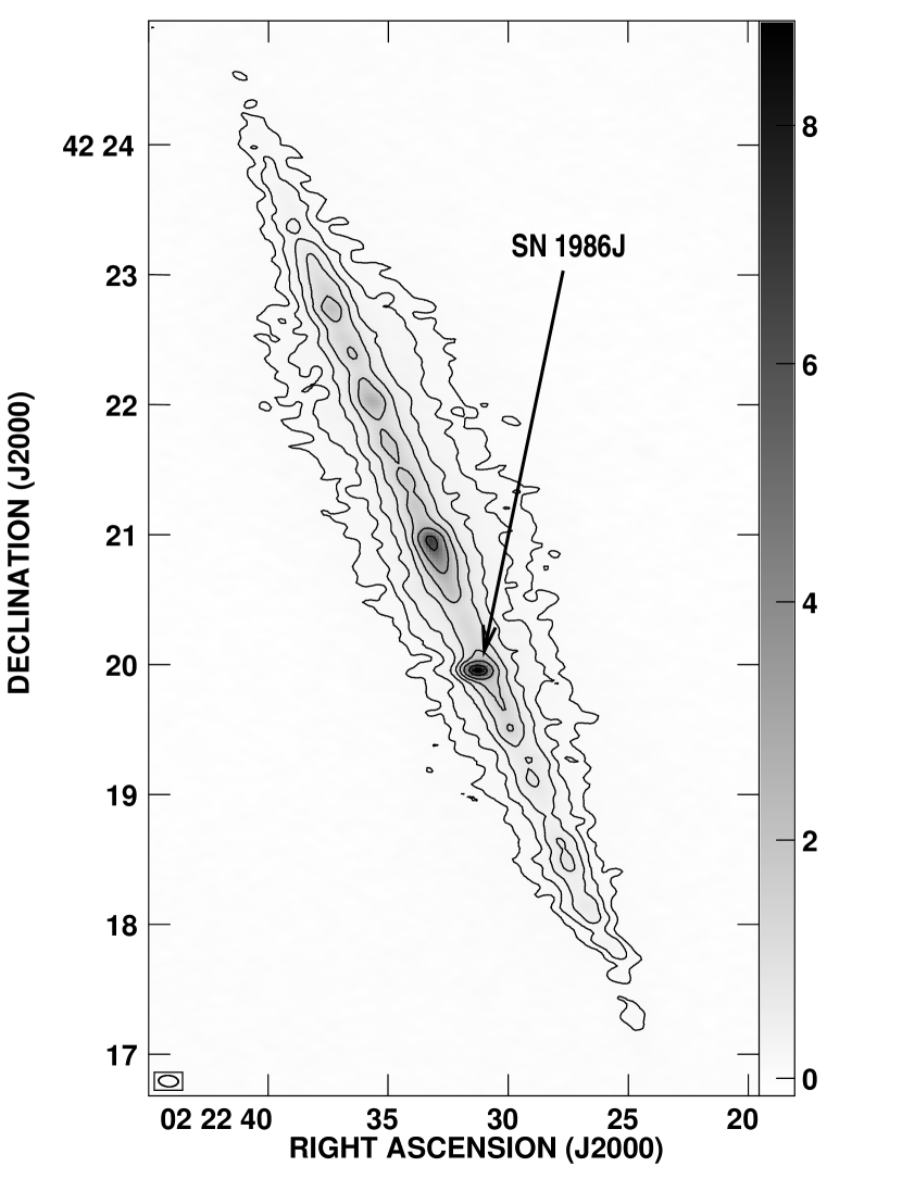
Figure 2: A VLA image of NCC 891 at 5.0 GHz on 1999 Feb. 22. The contours are drawn at 1, 2, 4, …, 64, and 90% of the peak brightness of 8.9 mJy beam^-1. The grayscale is labeled in mJy beam^-1. The rms of the background brightness was 33 $\mu$Jy beam^-1. The CLEAN beam is plotted at lower left, and its FWHM was $9.1\arcsec\times 5.7\arcsec$ at p.a. 86°. SN 1986J is indicated.

We imaged the radio emission of the galaxy NGC 891 at 5.0 GHz in 1999.1, and show the result in Figure 2. SN 1986J is located south-west of the galactic nucleus. We also obtained total flux densities of SN 1986J at several frequencies at each epoch. With the exception of the one at 43 GHz, these flux densities were derived from data which were self-calibrated in phase but not in amplitude.

For the standard error of the total flux density measurements, we take the sum in quadrature of the statistical standard error, an uncertainty in the VLA flux density calibration, and the additional systematic uncertainties detailed below. The uncertainty in the VLA flux density calibration was taken to be 5% for frequencies up to 14.5 GHz, 10% at 23.5 GHz, and 14% at 43 GHz (we use an uncertainty somewhat higher than usual at 43 GHz because of the aforementioned difficulty in amplitude calibration for that frequency). An additional systematic uncertainty arises because confusion needs to be taken into account for frequencies below 5 GHz at epoch 1999.1, for which the VLA was in the CnD configuration and the resolution was moderate. In particular, for these frequencies, we derive our flux densities from a combination of model-fits in the image plane and $u$-$v$ plane, with the contribution from the galactic core and disk of NGC 891 accounted for in the model-fits. In 1999.1 the brightness of NGC 891 was $\sim 2$ and $\sim 0.15$ times the peak brightness of SN 1986J at 1.5 and 5 GHz, respectively. The additional systematic uncertainty for these measurements is computed from the ambiguity of these model-fits. At 43 GHz, we take an additional systematic upward uncertainty of 50% because we could not self-calibrate in phase, and so may have underestimated the true flux density.

3 VLBI Images of SN 1986J

3.1 A High-Resolution Image at the Latest Epoch

In Figure 3, we show a 5-GHz image of SN 1986J at epoch 1999.1 made from our most sensitive observations using phase-referenced imaging. The image shows a rather complex extended radio source. The outer contours are very roughly circular, but the brightest point lies to the north-east of its apparent center. There is a minimum in the interior, which lies somewhat to the south-west of the apparent center. This structure could be interpreted as a shell, albeit a quite heavily modulated one. An optically thin, spherical shell of uniform volume emissivity would have a brightness distribution with a minimum in the center and a circular ridge-line which is close to its projected inner radius. The most prominent deviation of our image of SN 1986J from such a geometry is the prominent brightness peak to the north-east, which we label C1. The peak flux density per beam at the location of C1 is $\sim 1.6$ mJy.

As mentioned before, we also fit a geometrical model directly to the $u$-$v$ data. Our choice of model was motivated by the morphology of the above image, and our model consists of a spherical shell of uniform volume emissivity and a point source to represent C1. We defer the detailed discussion of these model fits to §6.1 below. However, we indicate in Figure 3 the inner and outer radii of the fit shell, and we take the center of the fit shell as origin of the coordinate system. The fit point source is also indicated on the figure. It has a flux density of $\sim 1$ mJy, which indicates that C1 is approximately twice as bright as the shell emission at that location. We can then estimate C1 to have $\sim 16$% of the total flux density in the image, and to have a brightness temperature $\gtrsim 3\times 10^{7}$ K.

It is clear that the brightness distribution of SN 1986J does not resemble that of the described model in detail. Even allowing for the presence of C1, the shell brightness is heavily modulated. Two other components are visible, a south-western component C2 and a north-north-western component C3, each having a brightness a third that of C1. They can be interpreted as being part of the ridge of the shell. In addition to the shell, and to C1, C2 and C3, there are protrusions which add to the complexity of the image and cause significant deviations from circularity of the outer contours.

C1 itself, while relatively compact, may well not be entirely pointlike. Comparing its contours to those of the CLEAN beam shows an extension both toward the geometric center, labeled C1*, and toward the inner radius of the fit shell to the south. While part of the emission of C1, in particular the extension to the south, can probably also be interpreted as being part of the ridge, the largest part of C1 is located rather further toward the geometric center than one might expect from a shell component, unless it is an unusually strong component located on the front of the shell.

Qualitatively, the structure of the supernova is similar to that found in 1988.7 by B91. The shell structure, only marginally discernible in the 1988.7 image, has now become somewhat clearer. A north-eastern component dominated the image at the early epoch and such a component still dominates the image in 1999.1. Protrusions distorted the image in 1988.7 and still characterize the appearance of the supernova in 1999.1. Apart from these general similarities however, clear differences in the structure of the supernova have developed over the years.

3.2 A Comparative Study of the Sequence of Images at the Three Epochs

To investigate the structural evolution of the supernova in more detail, we produced a sequence of images of SN 1986J at three consecutive epochs from 1988.7 to 1999.1, approximately $t=6$, 7, and 16 yr after shock breakout. To better search for possible changes in the images over the years we adopt a more conservative image reconstruction technique than that used for making the image in Figure 3. In particular, we adopt a weighting scheme for the correlated flux densities which increases the dynamic range of the images. Since residual calibration errors may be present in the data and need not scale with the thermal noise, we compressed the weights somewhat by weighting by the inverse of the thermal noise rms, rather than the usual inverse of the thermal noise variance. Then, we choose a beam size based on the 1999.1 image made using Briggs’ robust weighting scheme (Briggs, Schwab, & Sramek, 1999; Briggs, 1995), with the robustness parameter in AIPS set to zero to give the best trade-off between signal-to-noise ratio and minimized sidelobes. A Gaussian fit to the inner portion of the dirty beam produced with this weighting gives a CLEAN beam with a full-width at half-maximum (FWHM) of 2.06 mas $\times$ 1.04 mas at a p.a. of $-7$°.

The angular resolution of our observations were different for each epoch. Therefore, in order to minimize any bias in the comparison of the images that could be introduced by the convolution with an inconsistently changing CLEAN beam, we choose to convolve our three images with a CLEAN beam whose size evolves similarly to that of the supernova. In particular we choose a CLEAN beam whose size evolves as $t^{0.75}$, in anticipation of our results on the deceleration of the supernova expansion described in §7 below. In order to accommodate the somewhat different angles of elongation of the original beams, we increase the length of the minor axis of the beam so that in 1999.1 it is 1.40 mas. With such a dynamical CLEAN beam, the appearance of the supernova would essentially not change apart from a scaling factor if the supernova evolved self-similarly.

We show the sequence of images produced in this way in Figure 4. It clearly shows that the supernova is expanding. This sequence is only the second, after that for SN 1993J (e.g., Bietenholz et al., 2002; Bartel et al., 2000; Rupen et al., 1998; Marcaide et al., 1997), where the expansion of the supernova is so clearly visible. It also shows that the structure is changing with time.

We now follow the evolution of the structure in more detail. In the 1988.7 image, a strong component is located approximately in the center of the radio source. Comparing this component to the 50% contour of the CLEAN beam, it is clear that this component is significantly extended. Judging from the early high-resolution image of B91, it is a combination of the strong northern component and the shell emission, since a spherical shell would be barely resolved at the relatively coarse angular resolution we now use. Further, protrusions to the south-east and to the north-west are clearly visible. B91 note parenthetically that in their high-resolution image a faint, additional protrusion to the south-west might perhaps be present, but we cannot confirm it in our image. To determine the extent to which the morphology is dependent upon the self-calibration, we “self”-calibrated the image from 1988 using a scaled version of the 1999 image, and found no change in the gross morphology described above.

In 1990.6, the bright component still dominates the image. It is again clearly extended, and presumably again a combination of the strong northern component mentioned above and a contribution from the shell. In addition a second component to the south-east has developed. We think it could be component C2 and part of the ridge. The protrusion to the north-west is still visible. A protrusion to the south-east is also visible, but appears to have an orientation 30° further to the south than the protrusion seen in 1988.7. It is striking that a new protrusion seems to have appeared to the north-east.

By 1999.1, the bright component, now labeled C1, still dominates the image. This time however, the component is compact. We fit a model including a point source to represent this component directly to the $u$-$v$ data (§6.1 below). If we subtract the fit point source at the location of C1 from the image, we obtain the brightness distribution shown in the fourth panel, which is indeed more similar to the brightness distribution in the second panel. The bright inner part has rotated further, toward an angle of $\sim-60$°, and forms an arc that extends to C3 and C2 as part of the ridge, which is also seen in the high-resolution image in Figure 3. The north-west and south-east protrusions are still visible, but have become less pronounced and contribute only mildly to the distortion of the morphology.

Looking at the three images in a more comprehensive way, three main characteristics are apparent: 1) The shell structure appears to have become more prominent since it is not discernible in our first image but becomes clearer in the following two images. 2) The protrusions appear to have expanded more slowly than the rest of the source. In fact there is a possibility that they have a more erratic nature evolving on a time scale shorter than a couple of years. 3) The brightest component is clearly resolved in the first two images and has a peak flux density per beam of only 21 and 17% of the total flux density of the source, respectively. In the last image, however, it is much more compact and in addition more prominent, having a peak flux density per beam of 29% of the total flux density.

3.3 A Search for Polarized Emission

We also made images in Stokes parameters $Q$ and $U$ for the observations in 1999.1. We determined the antenna polarization parameters from the observations of 3C 66A. We did not detect any significant linear polarization for SN 1986J. The $3\sigma$ upper limit on the polarized brightness is 0.11 mJy beam^-1 for a beam FWHM of 1.8 mas $\times$ 0.9 mas. This limit corresponds to a fractional linear polarization of $<7.5$% for the peak of the image.

4 The Radio Light Curves and the Spectrum

From interferometric VLA observations, we determined the total flux densities at different frequencies for the epochs 1998.4, 1999.1, and 2002.4, and we list them in Table 2. To illustrate the evolution of the flux density with time, we plot our flux densities at 5 GHz, as well as those measured by WPS90, in Figure 5. The evolution of the flux density with time, $t$, after the explosion date, $t_{0}$, is usually parameterized as $S_{\nu}\propto(t-t_{0})^{\beta}$ for the period after the supernova has become optically thin. WPS90 fit a model to their flux density measurements at frequencies between 0.3 and 23 GHz, and determined that $\beta=-1.18^{+0.02}_{-0.04}$ for the period up to 1989. We plot their fit also in Figure 5. Our flux densities are significantly below the extrapolation of WPS90’s fit, indicating a much more rapid decay of the flux density as a function of time. In fact, the average value of $\beta$ at 5 GHz between WPS90’s last measurement in 1989.0 and our first measurement in 1998.4 is $-2.22\pm 0.08$.

We have flux density measurements from 1998 to 2002, and therefore we can determine the current rate of flux density decay. We plot our flux density measurements at 1.4 to 23 GHz as a function of time in Figure 6. We also determined $\beta_{\nu}$ separately at each frequency, $\nu$, with a weighted least-squares fit, and these fits are also indicated in the figure. The rate of decline is even more rapid than the average rate between 1989 and 1998, with $\beta_{\nu}$ ranging from $-2.7\pm 0.3$ at 8.4 GHz to $-3.5\pm 0.9$ at 23 GHz. The values of $\beta_{\nu}$ at our different observing frequencies from 1.4 to 23 GHz are consistent within the uncertainties, suggesting that between 1998 and 2002, there is no significant change with time in the radio spectrum, and that $\beta$ is in fact independent of frequency to within our measurement errors.

The flux densities in Table 2 show that there is a significant inversion in the spectrum above 10 GHz. This inversion suggests that the spectrum can be decomposed into two components, a “normal” component, with a negative spectral index, and an “inverted” component with a positive spectral index at least up to 23 GHz. To consistently determine both, $\beta$, assumed now to be independent of frequency, and the spectrum, we combined all our flux density measurements except the one at 43 GHz. Then we fit $\beta$ and the two power-law components of the spectrum by weighted least squares. We derived uncertainties on our fit parameters from a Monte Carlo simulation, varying all the flux density measurements within their respective uncertainties and using 4000 realizations. We note that this decomposition of the spectrum is probably not unique, but it illustrates the general behavior of the spectrum and allows us to accurately determine $\beta$.

We find that the fit value of $\beta$ is $-2.94\pm 0.24$ between 1998 and 2002. This value is significantly different from that measured up to 1989, indicating that the rate of flux density decay has increased substantially between 1989 and 1998. An increase with time of the rate of flux density decay has been seen for other supernovae, in particular for SN 1980K (Montes et al., 1998) and for SN 1993J for which a distinct decrease in $\beta$ from $\sim-0.7$ to $\lesssim-1.2$ was found $\sim 6.5$ yr after the explosion (Bartel et al., 2002).

In Figure 7, we plot our flux densities, all scaled with the fit value of $\beta$ to the epoch of our last VLBI image. We also plot the two component fit to the time-averaged spectrum up to 23 GHz, along with the normal and inverted components of the spectrum. The normal component has $S_{\rm 5\;GHz}=6.3^{+0.6}_{-1.1}$ mJy and $\alpha=-0.55^{+0.09}_{-0.16}$. The spectral index of the normal component is consistent within the uncertainties with the optically thin spectral index of $\alpha=-0.67^{+0.08}_{-0.04}$ determined by WPS90 for the period up to 1989. The inverted component has $S_{\rm 5\;GHz}=0.8^{+1.0}_{-0.4}$ mJy and $\alpha=+1.4^{+0.6}_{-0.4}$.

The significant inversion in the spectrum visible above 10 GHz has not been observed for any other supernova. It is likely due to an element of SN 1986J with an emission process very different from that of the shell. This inversion of the spectrum of SN 1986J is seen on two different observing dates, using different amplitude and phase calibrators. Neither of the phase calibrators shows any break in their spectrum (Fig. 1). We therefore think that the inversion cannot be ascribed to any anomaly in the calibration of the data.

Has the inversion of the spectrum been seen before in SN 1986J? An inversion of the spectrum was indeed seen earlier, in the fall of 1986, when the spectrum was unusually steep between 14.9 and 22.5 GHz, with $\alpha=-1.5\pm 0.3$ (WPS90), but slightly inverted between 90 and 250 GHz (Tuffs, Chini, & Kreysa, 1989). A subsequent measurement at 250 GHz made one year later by the same authors, however, showed a much lower flux density and no inversion, the spectrum between 5 and 250 GHz being consistent with a single power-law with $\alpha\sim-0.63$ (WPS90). WPS90 concluded that either a transient component of SN 1986J was responsible for the spectral inversion, or that the measurement by Tuffs et al. (1989) was in error. We note, though, that for the second half of 1988, WPS90 report a steep spectrum with $\alpha\simeq-0.67$ between 5 and 15 GHz, and a relatively flat spectrum, with $\alpha\sim-0.2\pm 0.2$ between 15 and 23 GHz. Such a flattening is compatible with the presence of an inverted component of the spectrum. Their data, however, do not support an inverted component with as large a fraction of the total flux density as we observed later. Perhaps the inverted component is highly variable. If so, our finding that $\beta$ is independent of frequency suggests that we fortuitously observed at a time when the inverted component showed the same rate of decay as the normal one. Although our fit to the flux density decay and to the spectrum up to 23 GHz had a Chi-squared per degree of freedom of 0.5, indicating an excellent fit, the spectral decomposition is likely not unique. Our measurement at 43 GHz suggests a high-frequency turnover in the spectrum near $\sim 23$ GHz. It is possible that the inverted component of the spectrum deviates significantly from a power law at or even below 23 GHz. At 23 GHz, the likely minimum brightness temperature associated with the inverted component of the spectrum is $3\times 10^{6}$ K, derived by assuming a size no larger than the size of the entire emission region in the 5 GHz VLBI image of 1999.1.

Can the inverted component of the spectrum be related to any particular feature in our images of SN 1986J? If the inverted component of the spectrum is related to a compact feature in the images, then the feature could be visible in our images. Based on our fit to the spectrum, we expect it to have $S_{\rm 5\;GHz}=0.8^{+1.0}_{-0.4}$ mJy in 1999.1. Since the rms of the background brightness in our 1999.1 VLBI image (Fig. 3) is only 40 $\mu$Jy beam^-1, such a feature should be visible. We note, however, that if the inverted component of the spectrum deviates from a power law below 23 GHz, the value of $S_{\rm 5\;GHz}$ could be in error. The most obvious candidate for the feature in the images is component C1, corresponding to the fit point source in our models, which has a flux density of $\sim 1$ mJy. Indeed, the compact component, C1, is dominant in the VLBI image of 1999.1 (Fig. 3), but is not apparent in that of 1988.7.

5 Astrometric Results

Phase referencing, which we did for our 1999.1 VLBI observations, allows the determination of accurate relative positions. In principle, the coordinates of the explosion center of a supernova can be determined accurately with VLBI astrometry relative to a suitable, stable, reference point nearby on the sky. The core of a galaxy or a quasar would be a suitable reference point: with present astrometric techniques, these cores have no detectable proper motion (e.g. Bartel et al., 1986), and can therefore be assumed for our purposes to be stationary. In particular, in the case of SN 1993J, we used phase-referenced imaging with respect to the core of the nuclear radio source of M81 to determine the explosion center of SN 1993J with an accuracy of 45 $\mu$as or 160 AU at the distance of the galaxy (Bietenholz, Bartel, & Rupen, 2001). This measurement allowed us to relate the expansion of the radio shell to the explosion center and to place limits on any anisotropy in the expansion of the supernova with high accuracy.

Our observations were made using the radio galaxy 3C 66A, which is only 42 arcmin away from SN 1986J, as a phase reference source. We display an image of 3C 66A in Figure 8. The source is characterized by a core component and a 20 mas long, one-sided jet to the south-southwest. As the reference point for our astrometric measurements, we used the position of the phase center of 3C 66A, which is essentially that of the peak of the brightness distribution. We also use this position as the origin of the coordinate system of the image in Figure 8. The position of this point is the a priori position of 3C 66A assumed for the correlation of the data. Its coordinates are R.A. = ${2}^{\rm h}\;{22}^{\rm m}\;{39}\fs{61148}$, decl. = ${+43}\arcdeg\;{02}\arcmin\;{7}\farcs{7993}$ (J2000). Relative to these coordinates, we determined that the coordinates of the center of SN 1986J were R.A. = ${2}^{\rm h}\;{22}^{\rm m}\;{31}\fs{3211}$ and decl. = ${+42}\arcdeg\;{19}\arcmin\;{57}\farcs{2820}$ (J2000).

The accuracy of these relative coordinates is limited by errors in the correlator model of the tropospheric and ionospheric delays, as well as of UT1, polar motion, and antenna coordinates to roughly 100 $\mu$as (see Bartel et al., 1986, for an estimate of such error for the close pair of quasars 3C 345 and NRAO 512). Furthermore, the brightness peak is not necessarily located at the core of the galaxy. It may depend on possible structure changes near the core (see e.g., Bietenholz, Bartel, & Rupen, 2000; Bartel et al., 1986). For instance, the brightness distribution of the nuclear radio source of M81 Bietenholz et al. (2000) varies on short timescales, as does that of many superluminal sources. Also the brightness distribution of the peak may be dependent on frequency and the size of the convolving beam. The brightness distribution of the central part of 3C 66A is approximately Gaussian at our resolution and frequency, with a major axis FWHM of $\sim 1$ mas. We therefore assume a provisional positional uncertainty of 1 mas in identifying the core or any related other stationary point in 3C 66A. Future observations, perhaps at several frequencies, will likely allow a more accurate location of the core.

These difficulties will have to be carefully considered in any future astrometric observations of SN 1986J where 3C 66A is used as a phase-reference source. Despite the difficulties, such observations have the potential to answer important questions concerning the symmetry of the expansion, the effect of the CSM, and location of the explosion center, and above all, the location and identification in the images of the possible compact component responsible for the spectral inversion.

6 Size Determinations

6.1 Size Measurements by Model-Fitting in the $u$-$v$ Plane

In order to determine the expansion velocity and possible deceleration of the radio source SN 1986J, we must estimate its size at each of our epochs. Given the complexity of the source and its changes with time, such estimates are not as straightforward as in case of the symmetric shell of SN 1993J. We restrict ourselves here to average measures of the shell radius. We begin by discussing measures derived by fitting geometrical models to the $u$-$v$ (visibility) data. Such model fits have the advantage of being independent of the bias introduced by convolving with a CLEAN beam, but they have the disadvantage of being dependent on the model, which can at best only approximately represent the complex structure of the supernova.

We fit the geometrical model by weighted least-squares directly to the calibrated $u$-$v$ data. The model we chose consisted of two components. The first component was the two-dimensional projection of a three-dimensional, spherical, optically thin shell of uniform volume emissivity. Since the shell was not sufficiently resolved to warrant also solving for its thickness, we fix the ratio of the outer to inner angular radius at $\mbox{$\theta_{\rm o}$}/\mbox{$\theta_{\rm i}$}=1.25$, similar to that which provided the best fit for the shell of SN 1993J (Bartel et al., 2002; Bietenholz et al., 2002). The second component was a point source, and was introduced to parameterize the prominent hot-spot visible to the north-west in the images (Figure 4; see also B91). Both the position and the flux density of the point source are free parameters. From these fits, we estimated $\theta_{\rm o}$ and give the results in Table 3.

The statistical standard errors of $\theta_{\rm o}$ are generally $<20$ $\mu$as or $<1$%. The true uncertainties of $\theta_{\rm o}$, however, are almost certainly dominated by systematic errors, in large part due to the problem of fitting a simple geometric model to the complex and evolving structure of SN 1986J. Other systematic errors, e.g., those due to the unknown shell thickness and to possible residual errors in the amplitude and phase calibration also contribute to the overall error budget (see Bartel et al., 2002, for a longer discussion of the uncertainties in a similar model-fitting process). To estimate the systematic errors we monitored the changes of the values of $\theta_{\rm o}$ at various stages in the self-calibration process and for various positions of nearby local minima in the $\chi^{2}$ space. We obtained a typical error of $\sim 70$ $\mu$as. To estimate how much the values of $\theta_{\rm o}$ depend on our choice of a suitable model for SN 1986J, we modified our model by deleting the point source. We found that the values of $\theta_{\rm o}$ changed by only $\sim 20$ $\mu$as for the epoch 1988.7 and virtually not at all for epoch 1990.6. For epoch 1999.1 the value changed by $\sim 160$ $\mu$as. Such relatively large change, coupled with a significant fit flux density of the point source, in contrast to the results of the previous two epochs (see also §3), indicates that the point source is an appropriate addition to the shell model, at least for the 1999.1 epoch. We varied our model further and added a second point source for epoch 1988.7, since a second strong southern compact component appears in the high-resolution image of B91, and found that the value of $\theta_{\rm o}$ decreased by only $\sim 20$ $\mu$as. In conclusion we adopt a standard error of 70 $\mu$as for the values of $\theta_{\rm o}$ at each of our three epochs.

6.2 Size Measurements in the Image Plane

Since the images do not show detailed agreement with the simple geometrical model, we also determined the size of the radio source SN 1986J in the image plane and in a fashion not dependent upon the assumption of a particular geometry. Since our goal is to estimate the expansion velocity and $m$, we need to use a consistent means of determining the sizes at different epochs. Measuring the size in the image plane has the advantage of being able to more accurately account for the complex structure of the shell, but the disadvantage that such measurements are biased by the convolution with the CLEAN beam (Bartel et al., 2002). In particular, a determination of the deceleration parameter, $m$, is sensitive to the choice of the CLEAN beam for each epoch. For example, using a CLEAN beam whose size increases linearly with time would bias the derived value of $m$ towards $m=1$. In general, any derived value of $m$ would be biased toward the corresponding value $m_{\rm beam}$, where the size of the CLEAN beam is $\propto t^{m_{\rm beam}}$. To limit the bias, we chose a dynamical CLEAN beam whose size evolves similarly to that of the supernova. As mentioned already in §3, we used a CLEAN beam whose FWHM evolves as $(t-t_{0})^{0.75}$ in anticipation of our later result for $m$ (see §7) with $t_{0}=1982.7$ (WPS90). We also used a CLEAN beam which evolved with $m=0.70$ and found no significant change in the results.

We derived two different kinds of radii from the images, the first referred to the images’ total flux density and the second to their peak brightness. The first kind of radius, $\theta_{\rm 90\%\;flux}$, is the equivalent radius of the area of the contour which contains 90% of the total flux density. The second kind of radius, $\theta_{\rm 10\%\;peak}$, is the equivalent radius of the area of the 10% contour of the images, that being the lowest “reliable” contour in the 1999.1 image, which has the smallest dynamic range. We list the values for the two kinds of radii in Table 3.

Determining the exact uncertainties of $\theta_{\rm 90\%\;flux}$ and $\theta_{\rm 10\%\;peak}$ is not straightforward, and as with the uncertainties of $\theta_{\rm o}$, they are likely dominated by systematic effects. However, they are probably comparable to those of $\theta_{\rm o}$. For instance, $\theta_{\rm 90\%\;flux}$ is only weakly dependent on the size of the convolving beam: when we changed the size of the beam by 10% in each dimension, we found that $\theta_{\rm 90\%\;flux}$ changed only by 3%. We further investigated how phase self-calibration would influence the measurement of $\theta_{\rm 90\%\;flux}$ for the case of the 1990.6 image: we found that $\theta_{\rm 90\%\;flux}$ before and after phase self-calibration was different by $<1$%. We thus think that the standard errors of $\theta_{\rm 90\%\;flux}$ and $\theta_{\rm 10\%\;peak}$ are indeed comparable to those of $\theta_{\rm o}$.

7 The Expansion Velocity, Explosion Date, and Deceleration

We can compute the average expansion velocity directly from our measurements of the average size. We note that the interpretation of the velocity so derived as a true expansion velocity rests on the implicit assumption that the synchrotron emission observed at our different epochs can be physically associated. We first use the radii, $\theta_{\rm 90\%\;flux}$, which are the measure of the average outer radius of the source least dependent on the source structure. Taking a distance of 10 Mpc, we obtain an expansion velocity between 1990.5 and 1999.1 of $6000\pm 800$ km s^-1.

To determine the date of explosion, the possible deceleration, and the velocity as a function of time, we again use the measurements of $\theta_{\rm 90\%\;flux}$. In addition to the measurements for our three epochs, we used earlier measurements of the size of SN 1986J. Two such measurements were reported by Bartel et al. (1989). They determined the parameters of an elliptical Gaussian fit to VLBI data at 10.7 GHz in 1987.1 and at 5.0 GHz in 1987.4. The geometric mean of the major and minor axes FWHM values was $1.37\pm 0.36$ and $1.26\pm 0.24$ mas, respectively.

In order to convert these measurements to values equivalent to $\theta_{\rm 90\%\;flux}$ we used the elliptical Gaussian fit to the data of epoch 1988.7 and computed the geometric mean of the FWHM for its two axes. Assuming that the ratio of $\theta_{\rm 90\%\;flux}$ and the geometric mean axis of the fit Gaussian in 1987.1 and 1987.4 would be the same as it was in 1988.7, we obtained two additional values that we used for the determination of $t_{0}$ and $m$. We list these values also in Table 3.

We also added to our set of data points the estimate of the explosion date, $t_{0}$, of $1982.7^{+0.8}_{-0.6}$ obtained from the radio light curves (WPS90) and give it a weight comparable to those of our size determinations. We determine the values of $t_{0}$, $m$, and $\theta_{\rm 1yr}$, the last being the angular radius of the supernova after 1 year, by fitting the function of the form $\theta_{\rm 1yr}(t-t_{0})^{m}$ to our values by weighted least squares. We plot the values of $\theta_{\rm 90\%\;flux}$ as well as the fit in Figure 9. Since the fit function is non-linear, and the fit parameters may not have Gaussian distributions, we derive the uncertainties from Monte Carlo simulations, varying each value of $\theta_{\rm 90\%\;flux}$ and the estimate of $t_{0}$ from the radio light curves according to their uncertainties, and using 4000 random permutations. This fit gives $t_{0}=1983.2^{+1.4}_{-1.1}$, $m=0.71\pm 0.11$, and $\theta_{\rm 1yr}=0.43^{+0.22}_{-0.13}$ mas. These values correspond to an expansion velocity at $t=5.5$ yr (1988.7) of 8100 km s^-1 and at $t=15.9$ yr (1999.1) of 5900 km s^-1.

It is not clear how closely $\theta_{\rm 90\%\;flux}$ can be associated with the average radius of the outer shock front. If, for example, the source were characterized by a pure shell morphology, then the radii, $\theta_{\rm o}$, would lead to a more direct estimate of the deceleration of the outer shock front. To explore our sensitivity to different definitions of the outer radius, we also calculated the value of $m$ from our two other kinds of radii, $\theta_{\rm o}$ and $\theta_{\rm 10\%\;peak}$.

For the epochs 1987.1 and 1987.4, we estimated the values of $\theta_{\rm o}$ and $\theta_{\rm 10\%\;peak}$ in the same fashion as we estimated $\theta_{\rm 90\%\;flux}$. From the fit for $\theta_{\rm o}$, we obtained $m=0.78\pm 0.11$, and for $\theta_{\rm 10\%\;peak}$ we obtained $m=0.60\pm 0.10$. The explosion date derived by WPS90 from the radio light curves is somewhat model dependent. If we omit their value from our fit to the values of $\theta_{\rm 90\%\;flux}$, we obtain $t_{0}=1986.2^{+0.7}_{-1.9}$, and $m=0.45^{+0.15}_{-0.08}$. Unfortunately, the VLBI size measurements alone do not well constrain the fit, and the parameters $m$ and $t_{0}$ are highly correlated, so our individual uncertainties on each are relatively large. The fit value of $t_{0}$ corresponds to a time of explosion somewhat, but not significantly, later than that of the first radio detection in 1984.4 (Rupen et al. 1987; van der Hulst et al. 1986). Similarly fitting the values $\theta_{\rm o}$ and $\theta_{\rm 90\%\;flux}$ gives $t_{0}=1984.7^{+1.9}_{-3.0}$, $m=0.62^{+0.24}_{-0.17}$ and $t_{0}=1986.1^{+1.2}_{-4.3}$, $m=0.38^{+0.26}_{-0.10}$, respectively.

All our fits give explosion dates somewhat later than WPS90’s value of 1982.7, suggesting that the true explosion date lies between that value and the first radio detection in 1984.4. All our values of $m$ indicate a moderate to strong deceleration. The best average value of $m$ is $0.71\pm 0.11$, obtained from $\theta_{\rm 90\%\;flux}$ with the inclusion of the estimate of $t_{0}$ from the light curves.

8 The Evolution of the Magnetic Field

Using synchrotron radiation theory (Pacholczyk, 1970), we can calculate the average magnetic field and infer its evolution. We use the measured radio light curve at 5.0 GHz, the spectral index of the normal component of the spectrum, and a source radius, $r_{\rm 90\%\;flux}$, which is the linear radius corresponding to $\theta_{\rm 90\%\;flux}$ at distance $D=10$ Mpc. We also assume that the energy distribution of the ultra-relativistic electrons in the interaction zone at any given time is a power law with $n(E)\propto E^{-\gamma}$, where $E$ is the electron energy, and $\gamma=1-2\alpha$. It can then be shown (e.g. Bartel et al., 2002) that the magnetic field, $B$, in Gauss, is

$$B=\left(6D^{2}{\zeta_{B}\over{\zeta_{\rm rel}fr^{3}_{\rm 90\%\;flux}}}\right)^{2\over\gamma+5}\left({{E_{\rm min}^{2-\gamma}S_{\nu}}\over{c_{5}(\gamma-2)}}\right)^{2\over\gamma+5}\left({\nu\over 2c_{1}}\right)^{\gamma-1\over\gamma+5},$$

with cgs units throughout. Here $u_{\rm rel}=\zeta_{\rm rel}u_{\rm e}$ and $u_{B}=\zeta_{B}u_{\rm e}$, where $u_{\rm e}$ is the internal thermal particle energy density, $u_{B}$ the magnetic field energy density with $u_{B}={B^{2}\over 8\pi}$, and $\zeta_{\rm rel}$, $\zeta_{B}$ are taken to be constants. Further, $f$, is the filling factor which accounts for the hollow interior of the radio shell, any irregularities in it, and for possible blocking of radiation from the rear of the shell, $E_{\rm min}$ is the minimum energy of the electrons, $c_{1}$ is a constant, and $c_{5}$ a function of $\gamma$ (the last two given in Pacholczyk, 1970).

For a constant spectral index, $\alpha=-0.67$, ${\zeta_{B}\over\zeta_{\rm rel}}=1$, $f=0.4$, $E_{\rm min}$ equivalent to 0.511 MeV, $\mbox{$r_{\rm 90\%\;flux}$}=2.0\times 10^{17}$ cm for $t=5.5$ yr (1988.7), $\mbox{$r_{\rm 90\%\;flux}$}\propto t^{m}$, and $S_{\nu}\propto t^{\beta}$, we can compute $B(t)$. Taking our value of $m$, which is relevant for the time interval 1983 to 1999, and taking $\beta=-2.22$, which was the average value between 1989 and 1999, and therefore best corresponds to our value of $m$, we get $B(t)=70\;(t/5.5\,{\rm yr})^{-1.2}$ mG.

We observed no significant polarization of the radio emission, and thus we cannot infer the geometry of the magnetic field from the direction of the radio polarization. However, the source size and the above estimates of the magnetic field imply sufficient internal Faraday rotation to completely depolarize the emission for any reasonable density in the radio shell.

9 Discussion

Three images of SN 1986J at consecutive epochs, 5.5, 7.4, and 15.9 years after the explosion have shown an expanding complex source that strongly evolves with time. SN 1986J is only the third supernova after SN 1993J (see e.g. Bartel et al. 2000, Bietenholz et al. 2001, for the latest sequence) and SN 1987A (Gaensler et al., 1997) for which a sequence of images could be made. The expansion is decelerated. Most interestingly, we found that the radio spectrum of SN 1986J is inverted above 10 GHz from 1999 to 2002, a characteristic generally absent in earlier radio spectra of SN 1986J, and not seen in any other supernova. The rate of flux density decay has increased substantially since 1989. The evolution with time, the change in the spectrum, and the change in the rate of flux density decay all clearly point to non-self-similar evolution for this source In the remainder we will discuss our findings in more detail.

9.1 The Extended Structure and its Evolution with Time

SN 1986J has a complex radio morphology that can be described as a shell or composite, with hot spots modulating the ridge, and protrusions piercing the rim, all evolving with time. These characteristics contrast with those of the highly circular radio shell of SN 1993J, but are similar to those of the compact source 41.95+575 in M82, which was believed to be a several-decades-old supernova remnant with a distorted shell (Bartel et al., 1987; Wilkinson & de Bruyn, 1990) although McDonald et al. (2001) suggest a different origin. The deceleration is moderate to strong, with the exact value of the deceleration parameter, $m$, depending on which definition of the radius is taken to determine it. The relatively large range from $m=0.60$ to 0.78 obtained for different types of radii suggests that even the evolution of the average radial profile of the supernova is not self-similar, since if it were, all consistent measures of the average radius should evolve with the same value of $m$. Nonetheless, all the values we obtained were consistent with our best-fit value of $0.71\pm 0.11$.

The radio light curve data suggest a strong change in the rate of flux density decay between 1989 and 1999. This change is likely to be accompanied by changes in $m$, as is seen in SN 1993J (Bartel et al., 2002). Our value of $m$ is the average value from the explosion time till 1999.1. It is possible, however, that $m$ was not constant during this interval, since our measurements are also consistent with an undecelerated expansion until $\sim 1992$, and a strong deceleration after that. Future size measurements are needed to constrain the current deceleration and to determine whether it is different from the average value.

Our best fit to the average deceleration, with $m=0.71$, corresponds to an expansion velocity in 1988.7 of $8100^{+1700}_{-830}$ km s^-1, about half the velocity of the outermost protrusion given by B91 after conversion to a distance of 10 Mpc. In 1988.7 the protrusions extended to twice the radius of the radio shell and had a mean velocity of 15,000 km s^-1. Unfortunately, it is not easy to track an individual protrusion between different epochs. In 1988.7 the two most prominent protrusions were at position angles, p.a., of $\sim-20\arcdeg$ and $\sim 110\arcdeg$. In 1990.6 the two most prominent protrusions were oppositely directed, at p.a. $\sim-20\arcdeg$ and $\sim 160\arcdeg$. However, in 1988.7, the south-east protrusion is only sharply pointed at the 27.5% contour. At lower contours the protrusion is rather broad, extending to the p.a. $\sim 160\arcdeg$. Perhaps it is the part of the protrusion near p.a. = 160° that grows to the protrusion seen in 1990.6. In addition, in 1990.6 a new protrusion appeared in the north-east. Perhaps the evolution of protrusions was somewhat erratic. In 1999.1 the structure of the supernova is more circular and protrusions are less prominent. They may have faded in emission or slowed.

If the protrusions have faded more rapidly than the remainder of the supernova, but still have the same relative extent that they did in 1989, then we may no longer be detecting the emission associated with the outer shock front. Consequently, the value of $m$ for the outer shock would in fact be larger than our value of 0.71, which was determined from average radii.

If the protrusions are slowing, for example because they are encountering a denser CSM, then they must be more strongly decelerated than the shell. We can calculate their deceleration by fixing $t_{0}$ at 1983.2 and measuring the lengths of the protrusions from the origin to the 90% flux density contour in the images $a)$, $b)$, and $d)$ in Figure 4, the last having the point source subtracted. We obtain a weighted mean $m$ for the protrusions of $\sim 0.6$. In this case, the protrusions are currently being overtaken by the shock front. Future measurements will show whether the deceleration of the shell also increases to $\sim 0.6$.

What is the origin of the deviations from circular symmetry in SN 1986J? The radio emission is thought to be generated by the interaction of the ejecta with the CSM which accelerates electrons to relativistic energies and amplifies the magnetic field. Anisotropies and irregularities in the velocity pattern or density profile of the ejecta, or in the density profile or magnetic field of the CSM could lead to a non-circular shock front or to a modulation of the brightness distribution along the ridge of the shell. In addition, Rayleigh-Taylor (R-T) instabilities are expected to develop because of the deceleration of the shock front, and also are also expected to cause distortions of the radio structure.

It is not easy to distinguish between these different influences on the radio structure of a supernova. Highly asymmetric ejecta could be caused by supersonic jets inducing the explosion of a supernova and then propagating outward in both polar directions (Khokhlov et al., 1999; Piran & Nakamura, 1987). Recently McDonald et al. (2001) noted that the compact source in M82, 41.95+575, which previously was similar to an elongated shell, now shows some characteristics of a bipolar outflow, perhaps matching the jet scenario. Other mechanisms that could cause asymmetries in the structure of a supernova discussed in the literature include the outbreak of plasma through weak points of the shell (Rees, 1987), and giant loops of magnetic field lines (Shklovskii, 1981). In the case of SN 1993J, spectropolarimetry gave evidence for an asymmetric density distribution in the ejecta (Trammell, Hines, & Wheeler, 1993). Hydrodynamical studies, however, have shown that the distortion of a supernova due to an axisymmetric density distribution in the ejecta was much smaller than the distortion for the complementary axisymmetric density distribution of the CSM (Blondin et al. 1996).

The complex structure could be largely due to influences of the CSM. The model-fits to the radio light curves suggest a clumpy medium, which could qualitatively explain some of the features of the radio structure of SN 1986J. Blondin, Lundqvist, & Chevalier (1996) studied the interaction of a supernova with an axisymmetric CSM density distribution having density enhancement at the rotational equator of the progenitor, and showed that such a distribution could form oppositely directed protrusions with lengths two to four times the radius of the shell. While we do see protrusions of this length, they do not seem to be always oppositely directed.

The growth of R-T fingers may also influence the structure of SN 1986J. Although the R-T fingers generally do not penetrate the outer shock to form protrusions, Jun, Jones, & Norman (1996) showed that the interaction of vortices with a clumpy CSM allows some of the fingers to grow beyond the outer shock. Such fingers might then be disrupted by the clumpy CSM and/or the conditions in the interaction region, leading to their diminishing prominence.

9.2 Synchrotron Self-Absorption at Early Times?

It has been suggested that synchrotron self-absorption is the dominant absorption mechanism early on in the evolution of a radio supernova (e.g. Slysh, 1990). Chevalier (1998) concluded on the basis of then available data on SN 1986J that, while synchrotron self-absorption was consistent with the low velocities determined from the H$\alpha$ emission, it was inconsistent with the large sizes and velocities determined through VLBI. He determined that, for synchrotron absorption to be significant, an outer radius of $<3.2\times 10^{16}$ cm was required at the peak of the 5-GHz light curve in 1986.3. We confirm the VLBI sizes measured in 1988, and our improved determination of the expansion velocity suggests a size in 1986.3 of 0.70 mas, corresponding to $1.1\times 10^{17}$ cm, three times larger than the maximum size for significant synchrotron self-absorption. The slow rise of the radio light curves is therefore likely due to effects other than synchrotron self-absorption, such as absorption within the emission region. As WPS90 pointed out earlier, such absorption would be consistent with filamentation of the radio shell structure and at least qualitatively with the complexity of our VLBI images.

9.3 The Swept-Up Mass and its Implications

The outer radius of SN 1986J in 1999.1 is 4.5$\times 10^{17}$ cm (calculated from $\theta_{\rm 90\%\;flux}$). For a value $\dot{M}/w$ of $2.4\times 10^{-4}$ $M_{\sun}$ yr^-1 per 10 km s^-1 inferred in part from the radio light curves (WPS90) we calculate that the total swept-up mass in 1999.1 would be $\sim 3.4$ $M_{\sun}$.

If we take the initial expansion velocity to be $\sim 20,000$ km s^-1, then momentum conservation suggests that the mass of the decelerated ejecta is $\sim 30$% that of the material swept up by 1999.1, or $\sim 1$ $M_{\sun}$. We can then estimate the total kinetic energy of the interaction region and the swept-up material to be $\sim 1.5$$\times 10^{51}$ ergs. The total kinetic energy in SN 1986J consists of that of the swept-up material, of the decelerated material, and of the still undecelerated inner ejecta. The kinetic energy in the undecelerated ejecta is probably $<10^{51}$ ergs, giving a total kinetic energy in the range of 1.5 to $\sim 2.5\times 10^{51}$ ergs. This is comparable to, or possibly somewhat larger than, the total kinetic energy estimated for a supernova explosion of a massive star, suggesting perhaps that the average value $\dot{M}/w$ is lower than given above. In fact, assuming that $\dot{M}/w$ is constant in time is equivalent to assuming $s=2$ (where $\mbox{$\rho_{\rm CSM}$}\propto r^{-s}$).

We can calculate $s$ within the context of the mini-shell model and self-similar evolution. In this model $s$ is related to the observables $m$, $\beta$ and $\alpha$ by $\beta=-(3-\alpha)(1-sm/2)+6m-\alpha m$ (Chevalier 1982a, b; see also Fransson, Lundqvist, & Chevalier 1996). Solving for $s$, we find $s=2.6$. We have shown that SN 1986J does not evolve in a self-similar fashion, so the model will not apply in detail. It does, however, seem likely that the external density profile is in fact steeper than $s=2$, at least for $t>5.5$ yr. A steeper profile is in agreement with the interpretation of recent X-ray results (Houck et al., 1998). This would imply on average a lower value of $\dot{M}/w$ than that determined early on by WPS90. Perhaps $\dot{M}/w$ was much smaller tens of thousands of years before the explosion and increased to the high value given by WPS90 only shortly before the star died.

9.4 Interpretation of the Inversion in the Spectrum

We found a clear inversion in the radio spectrum above 10 GHz (Fig. 7). The inverted part of the spectrum has a flux density which rises with frequency at least up to $\sim 23$ GHz, although there is likely a turnover or at least a flattening above that frequency.

The inversion in the spectrum suggests two distinct populations of relativistic electrons. The first is that of shock-accelerated electrons in the interaction region, which are responsible for the normal, uninverted component of the spectrum. The second is that responsible for the inverted component of the spectrum, and whose origin is unknown at this point. Since the flux density above 10 GHz is characterized by the same rate of flux density decay as seen at lower frequencies, the mechanism responsible for the inverted component of the spectrum is probably coupled to the expansion of the supernova, which drives the time-dependence of the normal component of the spectrum. The inverted part of the spectrum cannot then be due to a superposed HII region, which would not show any flux density decay. Accretion onto a compact object also often produces flat or inverted spectra, albeit not usually at such high radio luminosity for a stellar-mass object. A compact object is expected since the progenitor of SN 1986J was a massive star. Again, however, it seems unlikely that accretion onto the compact object would show the same time dependence as the emission from the expanding shell.

The inverted spectrum might be produced by either free-free or synchrotron self-absorption. Free-free absorption is characterized by a spectral index, $\alpha=+2.5$ and synchrotron self-absorption by $\alpha=+2.1$. Both absorption mechanisms would show a steep rise up to the frequency where the optical depth, $\tau_{\nu}$, is near unity, and then a turnover, provided the unabsorbed emission is characterized by $\alpha\lesssim+2$. If the source evolves, then $\tau_{\nu}$ and the spectrum are expected to change with time. In particular, if the source expands, $\tau_{\nu}$ would be expected to decrease, and the observed flux densities at frequencies where $\tau_{\nu}>0$ would be expected to increase relatively rapidly. This is in distinct contrast to our observation that the spectrum remained unchanged within the errors between 1999 and 2002, and that the flux density at all the observed frequencies decreased at the same rapid rate. This characteristic is puzzling and suggests that 1) $\tau_{\nu}$ remains relatively constant or even increases with time, and 2) the emission mechanism is coupled to the expansion of the supernova.

What is the absorption process? If the inversion of the spectrum is due to synchrotron self-absorption, we can compute the magnetic field, $B$, of the self-absorbed source and compare it with the equipartition field of the supernova. In particular, for a source like C1 with a FWHM $\lesssim 0.5$ mas, the flux density at 20 GHz of 5 mJy implies a magnetic field $B\gtrsim 2\times 10^{5}$ G. Such a field is seven orders of magnitude higher than the average equipartition field and therefore unlikely to be realized in a hot spot of the expanding shell. Given this characteristic coupled with points 1) and 2) above, it is unlikely that the inversion of the spectrum is due to synchrotron self-absorption. Could the inversion then be due to free-free absorption of the flat-spectrum emission of a pulsar nebula?

9.5 A Pulsar Nebula?

Already in 1988, B91 noted that the complex morphology of SN 1986J was not inconsistent with that of a shell with a weaker pulsar-wind nebula (PWN) in its center. We indicated in §4 above how a new, inverted component in the spectrum may be related to the compact feature C1 in our latest image, both of which were detected in 1999 but not previously.

Could this feature be a PWN? A PWN would only become visible once the optical depth of the interior of the shell had decreased to $\lesssim 1$, either through expansion or through fragmentation of the ejecta (Bandiera, Pacini, & Salvati, 1983). Since the putative PWN would just now be becoming visible, this suggests that the optical depth would just now have decreased to $\sim 1$. However, we argued in §9.4 above that the optical depth is, if anything, increasing with time, rather then decreasing as required by this interpretation.

If we nonetheless associate the image component C1 with the inverted component of the spectrum and with a putative PWN, then the latter’s flux density at 5 GHz is $\sim 1$ mJy. At 10 Mpc, this corresponds to a spectral luminosity $100\times$ that of the Crab Nebula. In agreement with the observed luminosity, Bandiera, Pacini, & Salvati (1984) calculated that a young PWN would have a luminosity 10 to 1000 times that of the Crab Nebula. They also calculated that the luminosity would decay with time, again consistent with our observations, although they do not find the decay to be as rapid as we have observed.

A PWN would be expected to be near the explosion center of SN 1986J, since pulsar velocities, typically $<500$ km s^-1, are much smaller than our observed expansion velocity of $>5000$ km s^-1. The component, C1, however, is located approximately half-way between the center and the perimeter of the source. It may be that the geometric center as determined either from the shell fit or the center of, say, the contour containing 90% of the flux density, is not the center of the explosion. The supernova’s structure is complex and the expansion may be anisotropic. In particular, the explosion center might be located close to C1. Only further phase-reference VLBI observations with accurate measurements of the proper motions of SN 1986J could shed more light on this possibility.

It may also be that a feature in the image closer to the geometric center is a candidate for the PWN. We note that a south-western extension of C1, labeled C1* on Figure 3, is much closer to the geometric center, and has a brightness of $\sim 0.3$ mJy. Again, further VLBI observations, preferably at high frequencies and phase referenced to 3C 66A, are needed to test the nature of this component.

10 Conclusions

Here we give a summary of our main conclusions.

1. The sequence of images of SN 1986J from 5.5 to 15.9 yr after the explosion is only the second such sequence, after that of SN 1993J, where the expansion and evolution is so clearly visible.

2. The sequence shows a complex source with a shell or composite morphology and protrusions that distort the perimeter of the supernova.

3. The structure of the supernova changes with time. The protrusions diminish somewhat in prominence, the shell structure becomes more visible, and a compact source with a flux density of $\sim 1$ mJy emerges half way between the perimeter and geometric center.

4. The spectrum shows a significant inversion above 10 GHz, which was not present before 1989. If the spectrum is composed of two power laws, the component with an inverted spectrum has a spectral index of $\alpha=+1.4^{+0.6}_{-0.4}$ below 23 GHz. The normal component of the spectrum has $\alpha=-0.55^{+0.09}_{-0.16}$, which is consistent with the value measured in 1989. Between 1998 to 2002, the spectrum remains relatively unchanged.

5. The inverted component of the spectrum or the image component C1 may be related to a pulsar nebula, but the current evidence is not conclusive.

6. The explosion date is estimated to be $1983.2\pm 1.1$, derived from both our expansion measurements and radio light curve modeling of others.

7. The expansion is found to be moderately to strongly decelerated, with the average outer radius being $\propto t^{0.71\pm 0.11}$ between $t=0$ and 15.9 yr. The expansion velocity in 1999.1 was 6000 km s^-1, only about one third of the extrapolated velocity after three months of $20,000$ km s^-1.

8. With the assumptions given, the average magnetic field is 70 mG at $t=5.5$ yr and declines $\propto t^{-1.2}$ between $t=5.5$ and 19.2 yr.

9. The flux density decreases $\propto t^{\beta}$ with $\beta=-2.94\pm 0.24$ from $t=15.9$ to 19.2 yr after the explosion. The rate of flux density decay increased substantially since $t=5.5$ yr, when $\beta$ was $-1.18^{+0.02}_{-0.04}$.

10. The changing structure, the emergence of an inverted part of the spectrum, and the change in the rate of flux density decay all clearly point out that the evolution of SN 1986J is not self-similar. Its evolution cannot be adequately described by self-similar solutions.

Table 1: VLBI Observations of SN 1986J

		ANTENNA																				Total	On-Source	Recording	Circular
Date	Freq.																					time	time	Mode	Polarization
	(GHz)	Eb	Mc	Nt	On	Go	Ro	Aq	Gb	Hs	Y	Br	Fd	Hn	Kp	La	Mk	Nl	Ov	Pt	Sc	(hr)	(baseline-hr)
1988 Sep 29	8.4	X			X	X	X		X	X	X								X*			12.3	071	III-A	R
1990 Jul 21	8.4	X			X	X	X	X	X	X	X											22.2	114	III-A	R
1999 Feb 22	5.0		X	X	X						X	X	X	X	X	X	X	X	X	X	X	11.8	266	256-8-2	R+L

Table 2: Total Flux Densities Measured at the VLA

Date	Freq.	Flux Density
	(GHz)	(mJy)
1998 June 5	1.67	$13.7\pm 0.9$
¨	4.99	$8.5\pm 0.5$
¨	8.41	$7.2\pm 0.4$
1999 Feb. 22	1.51	$15.0\pm 5.0$
¨	4.99	$7.3\pm 0.5$
¨	8.49	$6.1\pm 0.4$
¨	15.01	$8.1\pm 1.2$
¨	22.54	$9.5\pm 1.0$
2002 May 25	1.51	$7.1\pm 0.7$
¨	4.94	$4.2\pm 0.3$
¨	8.49	$3.8\pm 0.3$
¨	15.01	$7.1\pm 0.7$
¨	22.54	$5.0\pm 0.6$
¨	43.36	$3.9\;^{+\;2.1}_{-\;0.9}$

Table 3: Angular Radii for SN 1986J

Date	Age	Freq.	Model-fit radius	Image-plane radii
			$\theta_{\rm o}$	$\theta_{\rm 90\%\;flux}$	$\theta_{\rm 10\%\;peak}$
	(yr)	(GHz)	(mas)	(mas)	(mas)
1988 Sep. 29	5.55	8.4	$1.05\pm 0.07$	$1.34\pm 0.10$	$1.66\pm 0.12$
1990 July 21	7.35	8.4	$1.34\pm 0.07$	$1.91\pm 0.10$	$2.13\pm 0.12$
1999 Feb. 22	15.94	5.0	$2.33\pm 0.07$	$2.99\pm 0.10$	$3.14\pm 0.12$
1987 Feb. 23	3.95	10.7	$0.86\pm 0.23$	$1.08\pm 0.29$	$1.33\pm 0.36$
1987 May 30	4.21	5.0	$0.80\pm 0.15$	$1.01\pm 0.20$	$1.27\pm 0.24$

Figure 1: The radio spectra of the calibrator sources used for the VLA flux density observations. On 1999 February 22, the flux calibrator was 3C 286 and the secondary calibrator was 0230+405. On 2002 May 24 The flux calibrator was 3C 48 (except at 43 GHz, see text) and the secondary calibrator was 0303+472. We plot the adopted polynomial spectra for 3C 48 and 3C 286. The coefficients, as implemented in modern versions of AIPS, are (Perley, private communication) as follows, where $S_{\nu}$ is in Jy and $x$ is log($\nu$ in GHz). For 3C 286, $S_{\nu}=1.23734-0.43276x-0.14223x^{2}+0.00345x^{3}$, and for 3C 48, $S_{\nu}=1.31752-0.74090x-0.16708x^{2}+0.01525x^{3}$.

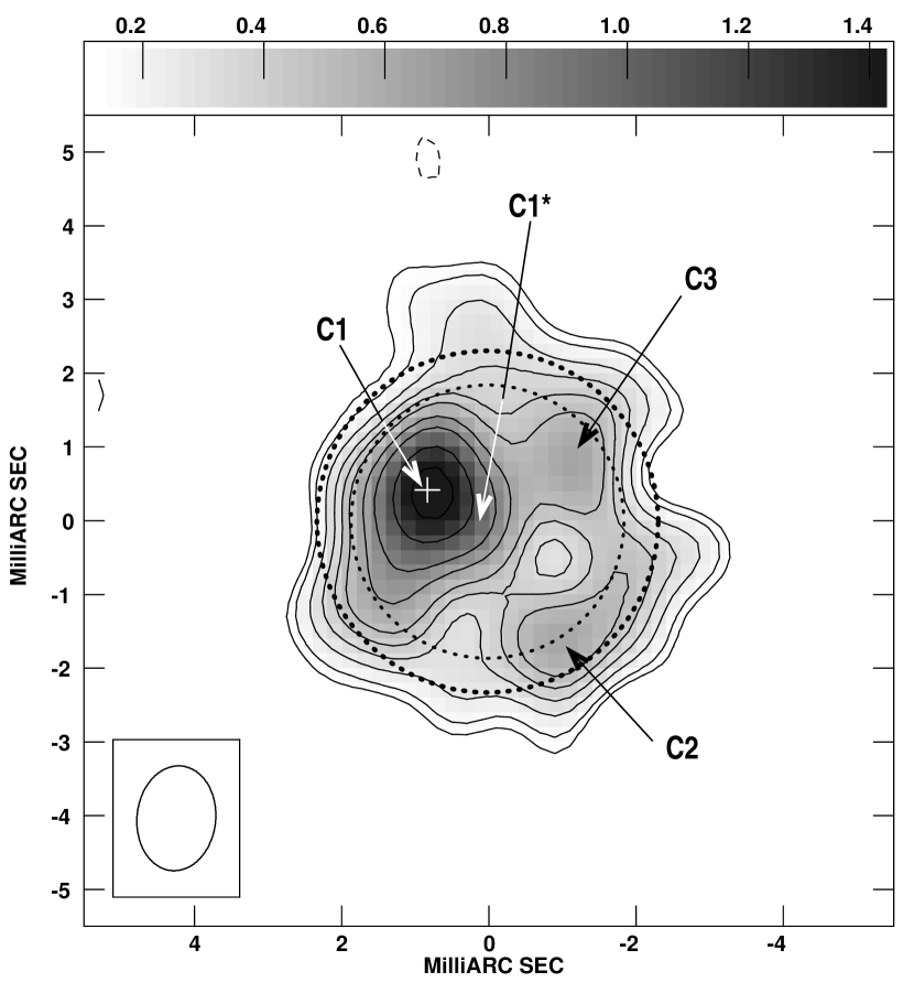
Figure 3: A high-resolution image of SN 1986J on 1999 February 22 at 5 GHz. The CLEAN beam was 1.42 mas $\times$ 1.07 mas FWHM at p.a. $=-5$° and is plotted at lower left. We chose the CLEAN beam to have the same area, but be somewhat more circular than an elliptical Gaussian fit to the inner portion of the dirty beam. Contours are drawn at $-7.4$, 7.4, 10, 15, 20, 25, 30, 40, 50, 70, and 90% of the peak brightness of 1.64 mJy beam^-1. The rms of the background brightness was 40 $\mu$Jy beam^-1. The dotted circles indicate the inner and outer radii of a spherical shell fit to the $u$-$v$ data (see text, §6.1). Note that the brightest portion of a projected shell of uniform volume emissivity is at the inner radius. The white cross indicates the position of the point source also fit to the data. North is up, and east is to the left.

Figure 4: Four images of SN 1986J. The epoch and frequency are given in the upper right corner of each panel. The first three are the images of SN 1986J at our three VLBI epochs. The fourth, shown for comparison, is the image in 1999.1 with the fit point source subtracted (see text, §6.1). The FWHM of the convolving beam, indicated at lower left in each panel, was chosen to evolve as $(t-1982.7)^{0.75}$. In all four panels, the lowest contour is drawn at $3\times$ the rms of the background brightness, and the heavier contour is the one which contains 90% of the total flux density in the image (see text, §6.2). For all images, north is up, and east is to the left.
$a$) 1988.7: the FWHM of the CLEAN beam was 1.0 mas $\times$ 0.66 mas at $-10$°; the contours are drawn at $-5$, 5, 8, 16, 27.5, 40, 50, 70, and 90% of the peak brightness of 7.9 mJy beam^-1.
$b$) 1990.5: the FWHM of the CLEAN beam was 1.2 mas $\times$ 0.81 mas at $-10$°; the contours are drawn at $-8$, 8, 17.6, 30, 40, 50, 70, and 90% of the peak brightness of 4.2 mJy beam^-1.
$c$) 1999.1: the FWHM of the CLEAN beam was 2.1 mas $\times$ 1.4 mas at $-10$°; the contours are drawn at 5, 8, 12.1, 30, … 90% of the peak brightness of 2.1 mJy beam^-1.
$d$) 1999.1: The CLEAN beam was as in $c)$. The contours are drawn at 11, 16, 20.7, 30, … 90% of the peak brightness of 1.0 mJy beam^-1. Note that the heavier contour is that which contains 90% of the flux density remaining after the point source has been subtracted.

Figure 5: The total flux density of SN 1986J as a function of time. Our measurements are plotted as filled circles. In addition we plot the values taken from WPS90, along with the fit radio light curve they derived from measurements between 0.3 and 22.5 GHz.

Figure 6: The total flux density of SN 1986J as measured with the VLA at various frequencies as a function of time. For clarity, some points have been shifted slightly in time. The lines indicate weighted fits to the flux density decay with time, with the relevant value of $\beta$ (i.e., slope) indicated. The standard errors include statistical and systematic contributions.

Figure 7: The spectrum of SN 1986J as measured with the VLA. Some points have been shifted slightly in frequency for clarity. The solid line indicates a weighted, two-component fit to the spectrum up to 23 GHz and the flux density decay. The measurements in 1998 and 2002 were scaled to epoch 1999 using the fit value of $\beta$ of $-2.94$. The dotted lines illustrate the two power-law components of the fit spectrum, which have the indicated spectral indices, $\alpha$.

Figure 8: A naturally weighted image of the source 3C 66A, which was used as a phase-reference source. The origin is at the phase center of 3C 66A: R.A. = ${2}^{\rm h}\;{22}^{\rm m}\;{39}\fs{61148}$, decl. = ${+43}\arcdeg\;{02}\arcmin\;{7}\farcs{7993}$ (J2000). Contours are drawn at 0.5, 1, 2, 4, 8, 15, 30, 50, 70, and 90% of the peak brightness of 0.69 Jy beam^-1, with the 50% contour being emphasized. The FWHM of the CLEAN beam, indicated at lower left, was 3.8 mas $\times$ 3.5 mas at p.a. $=-11$°. North is up, and east is to the left.

Figure 9: The expansion of SN 1986J as a function of time. We plot the angular radius, $\theta_{\rm 90\%\;flux}$, against the year. The line indicates an expansion of the form $\theta\propto(t-t_{0})^{m}$, with $m=0.71$ and $t_{0}=1983.2$, which are the values derived from our best fit (see text §7).

References

- Aaronson et al. (1982) Aaronson, M., et al. 1982, ApJS, 50, 241
- Baars et al. (1977) Baars, J. W. M., Genzel, R., Pauliny-Toth, I. I. K., & Witzel, A. 1977, A&A, 61, 99
- Bandiera, Pacini, & Salvati (1983) Bandiera, R., Pacini, F., & Salvati, M. 1983, A&A, 126, 7
- Bandiera, Pacini, & Salvati (1984) Bandiera, R., Pacini, F., & Salvati, M. 1984, ApJ, 285, 134
- Bartel et al. (1986) Bartel, N., Herring, T. A., Ratner, M. I., Shapiro, I. I., & Corey, B. E. 1986, Nature, 319, 733
- Bartel et al. (1987) Bartel, N., Ratner, M. I., Rogers, A. E. E., Shapiro, I. I., Bonometti, R. J., Cohen, N. L., Gorenstein, M. V., Marcaide, J. M., & Preston, R.A. 1987, ApJ, 323, 505
- Bartel et al. (1991) Bartel, N., Rupen, M. P., Shapiro I. I., Preston, R. A., & Rius, A. 1991, Nature, 350, 212, (B91)
- Bartel, Shapiro & Rupen (1989) Bartel, N., Shapiro, I. I., & Rupen, M. P. 1989, ApJ, 337, 85
- Bartel et al. (2000) Bartel, N., et al. 2000, Science, 287, 112
- Bartel et al. (2002) Bartel, N. et al., 2002, submitted to ApJ
- Bietenholz, Bartel, & Rupen (2000) Bietenholz, M. F., Bartel, N., & Rupen, M. P. 2000, ApJ, 532, 895
- Bietenholz, Bartel, & Rupen (2001) Bietenholz, M. F., Bartel, N., & Rupen, M. P. 2001, ApJ, 557, 770
- Bietenholz et al. (2001) Bietenholz, M. F., et al. 2001, in IAU Symposium 205: Galaxies and Their Constituents at the Highest Angular Resolution, ed. R. T. Schilizzi, S. Vogel, F. Paresce & M. Elvis, (San Francisco: ASP), 380
- Bietenholz et al. (2002) Bietenholz, M. F., et al. 2002, in preparation
- Blondin, Lundqvist, & Chevalier (1996) Blondin, J. M., Lundqvist, P., & Chevalier, R. A. 1996, ApJ, 472, 257
- Briggs (1995) Briggs, D. S. 1995, High Fidelity Deconvolution of Moderately Resolved Sources, (PhD. Thesis), NRAO
- Briggs, Schwab, & Sramek (1999) Briggs, D. S., Schwab, F. R., & Sramek, R. A. 1999, in Synthesis Imaging in Radio Astronomy II, ASP Conference Series, vol. 180, ed. G. B. Taylor, C. L. Carilli, & R. A. Perley (San Francisco: ASP), 127
- Chevalier (1982a) Chevalier, R. A. 1982, ApJ, 258, 790
- Chevalier (1982b) Chevalier, R. A. 1982, ApJ, 259, 302
- Chevalier (1987) Chevalier, R. A. 1987, Nature, 329, 611
- Chevalier (1998) Chevalier, R. A. 1998, ApJ, 499, 810
- Chugai (1993) Chugai, N. N. 1993, ApJ, 414, L101
- Ferrarese et al. (2000) Ferrarese, L. et al. 2000, ApJ, 529, 745
- Fransson, Lundqvist, & Chevalier (1996) Fransson, C., Lundqvist, P., & Chevalier, R. A. 1996, ApJ, 461, 993
- Gaensler et al. (1997) Gaensler, B. M., et al. 1997, ApJ, 479, 845
- Houck et al. (1998) Houck, J. C., Bregman, J. N., Chevalier, R. A., & Tomisaka, K. 1998, ApJ, 493, 431
- Jun, Jones, & Norman (1996) Jun, B-I., Jones, T. W., & Norman, M. L. 1996, ApJ, 468, L59
- Khokhlov et al. (1999) Khokhlov, A. M., Höflich, P. A., Oran, E. S., Wheeler, J. C., Wang, L., & Chtchelkanova, A. Yu. 1999, ApJ, 524, L107
- Kraan-Korteweg, (1986) Kraan-Korteweg, R. C. 1986, A&A Suppl., 66, 255
- Leibundgut et al. (1991) Leibundgut, B., Kirshner, R. P., Pinto, P. A., Rupen, M. P., Smith, R. C., Gunn, J. E., & Schneider, D. P. 1991, ApJ, 372, 531
- Linfield (1986) Linfield, R. P. 1986, AJ, 92, 213
- Massi & Aaron (1999) Massi, M., & Aaron, S. 1999, A&ASuppl., 136, 211
- Marcaide et al. (1997) Marcaide J. M., et al. 1997, ApJ, 486, L31
- McDonald et al. (2001) McDonald A. R., Muxlow, T. W. B., Pedlar, A., Garrett, M. A., Wills, K. A., Garrington, S. T., Diamond, P. J., & Wilkinson, P. N. 2001, MNRAS, 322, 100
- Mioduszewski, Dwarkadas, & Ball (2001) Mioduszewski, A. J., Dwarkadas, V. V., Ball, L. 2001, ApJ, 562, 869
- Montes et al. (1998) Montes, M. J., Van Dyk, S. D., Weiler, K. W., Sramek, R. A., & Panagia, N. 1998, ApJ, 506, 874
- Pacholczyk (1970) Pacholczyk, A. G. 1970, Radio Astrophysics (San Francisco: Freeman)
- Piran & Nakamura (1987) Piran, T., & Nakamura, T. 1987, Nature, 330, 28
- Rees (1987) Rees, M. 1987, Nature, 328, 207
- Rupen, Bartel, & Foley (1991) Rupen, M. P., Bartel, N., & Foley, A. R. 1991, in SN 1987A and other Supernovae, eds. I. J. Danziger and K. Kjär, (Garching: ESO), 645
- Rupen et al. (1987) Rupen, M. P., van Gorkom, J. H., Knapp, G. R., Gunn, J. E., & Schneider, D. P. 1987, AJ, 94, 61
- Rupen et al. (1998) Rupen, M. P., et al. 1998, IAU Coll. 164, Astr. Soc. Pac. Conf. Ser., ed. J. A. Zensus, G. B. Taylor & J. M. Wrobel (San Francisco), 144, 355
- Shklovskii (1981) Shklovskii, I. S. 1981, Soviet Astr. Letters, 7, 263
- Slysh (1990) Slysh, V. I. 1990, Soviet Astr. Letters, 16, 339
- Stathakis & Sadler (1991) Stathakis, R. A., & Sadler, E. M. 1991, MNRAS, 250, 786
- Tonry et al. (2001) Tonry, J. L., Dressler, A., Blakeslee, J. P., Ajhar, E. A., Fletcher, A. B., Luppino, G. A., Mezger, M. R., & Moore, C. B. 2001, ApJ, 546, 681
- Trammell, Hines, & Wheeler (1993) Trammell, S. R., Hines, D. C., & Wheeler, J. C. 1993, ApJ, 414, L21
- Tuffs, Chini, & Kreysa (1989) Tuffs, R. J., Chini, R., & Kreysa, E. 1989, in Proc. 22nd ESA Symposium: IR Spectroscopy (ESA SP-290) eds. A. C. H. Glasse, M. F. Kessler, and R. Gonzalez-Riesta, 387
- Tully (1988) Tully, R. B. 1988, Nearby Galaxies Catalogue (Cambridge: Cambridge University Press)
- van der Hulst, de Bruyn, & Allen (1986) van der Hulst, J. M., de Bruyn, A. G., & Allen, R. (assumed authors) 1986, IAU Circ. No. 4258
- van Gorkom et al. (1986) van Gorkom, J. J., Rupen, M. P., Knapp, G., & Gunn, J. 1986, IAU Circ. No. 4248
- Walker (1999) Walker, R. C. 1999 in ASP Conf. Proc. 180, Synthesis Imaging in Radio Astronomy II, ed. G. B. Taylor, C. L. Carilli, and R. A. Perley (San Francisco: ASP), 274
- Weiler, Panagia, & Sramek (1990) Weiler, K. W., Panagia, N., & Sramek, R. A. 1990, ApJ, 364, 611, (WPS90)
- Weiler et al. (1986) Weiler, K. W., Sramek, R. A., Panagia, N., van der Hulst, J. M., & Salvati, M. 1986, ApJ, 301, 790.
- Wilkinson & de Bruyn (1990) Wilkinson, P. N., & de Bruyn, A. G. 1990, MNRAS, 242, 529