Observational Implications of a Plerionic Environment for Gamma-Ray Bursts

Abstract

We consider the possibility that at least some GRB explosions take place inside pulsar wind bubbles (PWBs), in the context of the supranova model, where initially a supernova explosion takes place, leaving behind a supra-massive neutron star (SMNS), which loses its rotational energy on a time scale of months to tens of years and collapses to a black hole, triggering a GRB explosion. The most natural mechanism by which the SMNS can lose its rotational energy is through a strong pulsar type wind, between the supernova and the GRB events, which is expected to create a PWB. We analyze in some detail the observational implications of such a plerionic environment on the afterglow and prompt GRB emissions, as well as the prospect for direct detection of the plerion emission. We find that for a simple spherical model, GRBs with iron lines detected in their X-ray afterglow should not have a detectable radio afterglow, and should have small jet break times and non-relativistic transition times, in disagreement with observations for some of the GRBs with X-ray lines. These discrepancies with the observations may be reconciled by resorting to a non-spherical geometry, where the PWB is elongated along the polar axis. We find that the emission from the PWB should persist well into the afterglow, and the lack of detection of such a component provides interesting constraints on the model parameters. Finally, we predict that the inverse Compton upscattering of the PWB photons by the relativistic electrons of the afterglow (external Compton, EC) should lead to high energy emission during the early afterglow that might explain the GeV photons detected by EGRET for a few GRBs, and should be detectable by future missions such as GLAST.

1 Introduction

The leading models for Gamma-Ray Bursts (GRBs) involve a relativistic wind emanating from a compact central source. The prompt gamma-ray emission is usually attributed to energy dissipation within the outflow itself, due to internal shocks within the flow that arise from variability in its Lorentz factor, while the afterglow emission arises from an external shock that is driven into the ambient medium, as it decelerates the ejected matter (Rees & Mészáros 1994; Sari & Piran 1997). In this so called ‘internal-external’ shock model, the duration of the prompt GRB is directly related to the time during which the central source is active. The most popular emission mechanism is synchrotron radiation from relativistic electrons accelerated in the shocks, that radiate in the strong magnetic fields (close to equipartition values) within the shocked plasma. An additional radiation mechanism that may also play some role is synchrotron self-Compton (SSC), which is the upscattering of the synchrotron photons by the relativistic electrons, to much higher energies.

Progenitor models of GRBs are divided into two main categories. The first category involves the merger of a binary system of compact objects, such as a double neutron star (NS-NS, Eichler et al. 1989), a neutron star and a black hole (NS-BH, Narayan, Pacyński & Piran 1992) or a black hole and a Helium star or a white dwarf (BH-He, BH-WD, Fryer & Woosley 1998; Fryer, Woosley & Hartmann 1999). The second category involves the death of a massive star. It includes the failed supernova (Woosley 1993) or hypernova (Pacyński 1998) models, where a black hole is created promptly, and a large accretion rate from a surrounding accretion disk (or torus) feeds a strong relativistic jet in the polar regions. This type of model is known as the collapsar model. An alternative model within this second category is the supranova model (Vietri & Stella 1998), where a massive star explodes in a supernova and leaves behind a supra-massive neutron star (SMNS) which on a time scale of a few years loses its rotational energy and collapses to a black hole, triggering the GRB event. Long GRBs (with a duration $\gtrsim 2\;{\rm s}$) are usually attributed to the second category of progenitors, while short GRBs are attributed to the first category. In all the different scenarios mentioned above, the final stage of the process consists of a newly formed black hole with a large accretion rate from a surrounding torus, and involve a similar energy budget ($\lesssim 10^{54}\;{\rm ergs}$).

In this work we perform a detailed analysis of the supranova model, focusing on its possible observational signatures. This aims towards establishing tools that would enable us to distinguish between the supranova model and other progenitor models through observations, and to constrain the model parameter using current observations. The original motivation for the supranova model was to provide a relatively baryon clean environment for the GRB jet. As it turned out, it also seemed to naturally accommodate the later detection of iron lines in several X-ray afterglows (Lazzati, Campana, & Ghisellini 1999; Piro et al. 2000; Vietri et al. 2001).

It was later suggested that the most natural mechanism by which the SMNS can lose its rotational energy is through a strong pulsar type wind, between the supernova and the GRB events, which typically creates a pulsar wind bubble (PWB), also referred to as a plerion (Königl & Granot 2002, KG hereafter; Inoue, Guetta & Pacini 2002, IGP hereafter). KG suggested that the shocked pulsar wind into which the afterglow shock propagates in this picture may naturally account for the large inferred values of $\epsilon_{e}\sim 0.1$ and $\epsilon_{B}\sim 10^{-3}-0.1$ (the fractions of the internal energy in the electrons and in the magnetic field, respectively) that are inferred from fits to afterglow observations (Wijers & Galama 1999; Granot, Piran & Sari 1999; Chevalier & Li 2000; Panaitescu & Kumar 2002). This is attributed to the fact that pulsar winds are believed to largely consist of electron-positron pairs, and have magnetization parameters in the right range. This relaxes the need of generating strong magnetic fields in the shock itself, as is required in other models, where the magnetic field in the external medium (assumed to be either the ISM or a stellar wind of a massive star progenitor) is typically too small to account for the values of $\epsilon_{B}$ that are inferred from observations. Another attractive feature of this model, pointed out by IGP is the possible high energy emission, in the GeV-TeV range, that may result from the upscattering of photons from the plerion by the relativistic electrons in the afterglow shock (external Compton, EC hereafter), and may be detected by GLAST. They have shown that the EC emission can provide a viable explanation for the extended GeV emission seen by EGRET in GRB 940217 (Hurley et al. 1994).

We use a simple spherical model for the PWB. We find that a spherical model cannot accommodate the typical afterglow emission together with the iron line features observed in the X-ray afterglow of some GRBs. However, it was mentioned early on that in order to have a long lived afterglow emission together with the iron line features, a deviation from spherical symmetry is needed, where the line of sight is relatively devoid of the material producing the iron lines (Lazzati et al. 1999; Vietri et al. 2001). This is required in order to avoid a direct collision of the afterglow shock with the line producing material on an observed time of the order of a day or so. It was later pointed out that a PWB is expected to exist inside the SNR shell, which decelerates the afterglow shock at a smaller radius, so that in order for the afterglow to remain relativistic up to a month or more, and produce the iron lines, we need the PWB to be elongated along its rotational axis (KG). In this paper we strengthen this conclusion, and show that in order to produce iron lines with a spherical PWB, its radius must be sufficiently small, resulting in a large density inside the PWB and a high self absorption frequency implying no radio afterglow, in contrast with observations. We leave the detailed treatment of an elongated PWB to a future work, while in the present work we briefly comment about the expected effects of an elongated geometry compared to a spherical one.

In this work we extend the analysis of KG and IGP, and perform detailed calculations of the radiation from the PWB, the prompt GRB and from the afterglow that occur inside the PWB. We now give a short overview of the structure of the paper, where in each section we stress the original features, new results and the observational constraints on the model. In §2 we present our “PWB” model, introduce the relevant parameterization and model the acceleration of the supernova remnant (SNR) shell by the shocked pulsar wind. We use a simple spherical geometry and the pulsar wind is assumed to consist of proton and $e^{\pm}$ components with roughly equal energies, as well as a magnetic field. The conditions under which the iron line features that were observed in several X-ray afterglows may be reproduced within the PWB model, are investigated in §3. We find that this requires a time delay of $\lesssim 1\;$yr between the supernova and the GRB events. In §4 we perform a detailed study of the plerion emission, including the synchrotron and SSC components, and provide an elaborate description of the relevant Klein-Nishina effect. We also discuss the upper cutoff that is imposed on high energy photons due to pair production with the radiation field of the PWB, go over the prospect for direct detection of the plerion emission, and derive observational constraints on the parameters of our model. The effects of the PWB environment on the prompt GRB emission are analyzed in §5, and we find that the EC from the prompt GRB should typically be very small, but might be detectable for extreme parameters. In §6 we discuss the implications of a plerionic environment on the afterglow emission, and introduce the appropriate parameterization. The radial density profile of the PWB is approximated as a power law in radius (KG), $\propto r^{-k}$, where $k$ typically ranges between $0$ (similar to an ISM) and $1$ (intermediate between an ISM and a stellar wind). The synchrotron, SSC and EC components are calculated and we provide detailed expressions for the break frequencies and flux normalization, for $k=0,\,1$. We also calculate the high energy emission that is predicted in this model. The results are discussed in §7 and in §8 we give our conclusions.

2 The Pulsar Wind Bubble

Within the framework of the supranova model, a SMNS (also simply referred to as a pulsar) is formed in a supranova explosion, and then loses a large part of its rotational energy before collapsing to a black hole and triggering the GRB. The most plausible mechanism for this energy loss is through a pulsar type wind (KG; IGP). A pulsar wind bubble (PWB) is formed when the relativistic wind (consisting of relativistic particles and magnetic fields) that emanates from a pulsar is abruptly decelerated (typically, to a Newtonian velocity) in a strong relativistic shock, due to interaction with the ambient medium. When a bubble of this type expands inside a SNR, it gives rise to a plerionic SNR, of which the Crab and Vela remnants are prime examples. Motivated by previous works (Rees & Gunn 1974; Kennel & Coroniti 1984; Emmering & Chevalier 1987; KG) we consider in detail a spherical model where the shocked pulsar wind remains largely confined within the SNR. In §7 briefly discuss the possible consequences of some more complicated geometries.

The wind luminosity may be estimated by the magnetic dipole formula (Pacini 1967),

$$L_{w}={B_{*}^{2}R_{*}^{6}\Omega_{*}^{4}\over 6c^{3}}=7.0\times 10^{44}\left({B_{*}\over 10^{12}\ G}\right)^{2}\left({R_{*}\over 15\,{\rm km}}\right)^{6}\left({\Omega_{*}\over 10^{4}\ {\rm s}^{-1}}\right)^{4}\ {\rm ergs\ s^{-1}}\,,$$ (1)

where $B_{*}$ is the polar surface magnetic field, $R_{*}$ is the circumferential radius (neglecting the distinction between its equatorial and polar values in this approximation), and $\Omega_{*}$ is the (uniform) angular velocity (whose maximum value is $\sim 2\times 10^{4}\ {\rm s}^{-1}$; e.g., Haensel, Lasota, & Zdunik 1999). The spin-down time of a rapidly rotating SMNS can be estimated as

$$t_{\rm sd}={E_{\rm rot}\over L_{w}}\approx 6\left({\alpha\over 0.5}\right)\left({M_{*}\over 2.5\,M_{\odot}}\right)^{2}\left({R_{*}\over 15\ {\rm km}}\right)^{-6}\left({\Omega_{*}\over 10^{4}\ {\rm s}^{-1}}\right)^{-3}\left({B_{*}\over 10^{12}\ {\rm G}}\right)^{-2}\ {\rm yr}$$ (2)

(see Vietri & Stella 1998), where $E_{\rm rot}=\alpha GM_{*}^{2}\Omega_{*}/2c$ is the portion of the rotational energy of an SMNS of mass $M_{*}$ and angular velocity $\Omega_{*}$ that needs to be lost before it becomes unstable to collapse. The spindown timescale, that sets the time delay between the supernova and GRB events, depends on the physical parameters of the SMNS. Of these parameters, the least constrained is the magnetic field, which is typically expected to be in the range of $\sim 10^{12}-10^{13}\;{\rm G}$, and may cause a variation of $\gtrsim 2$ orders of magnitude in $t_{\rm sd}$. There is also a strong dependence on the radius $R_{*}$, which depends on its mass $M_{*}$ and the (uncertain) equation of state, that may account for a change of up to $\sim 1$ order of magnitude in the scaling of $t_{\rm sd}$. For example, for $R_{*}=10\;{\rm Km}$, with the values of the other parameters as given in Eq. (2), we have $t_{\rm sd}\approx 60\;{\rm yr}$. We conclude that the expected range of $t_{\rm sd}$ is from a few weeks to several years.

During $t_{\rm sd}$ the luminosity of the wind is roughly constant and the wind should energize the PWB depositing an energy of the order of $E_{\rm rot}$. The luminosity of the pulsar wind is divided between its different components: fractions $\xi_{e}$, $\xi_{p}$, and $\sigma_{w}$ in $e^{\pm}$ pairs, protons and Poynting flux (magnetic field), respectively. The inferred values of $\xi_{B}=\sigma_{w}/(1+\sigma_{w})$ for PWBs, such as Vela or the Crab, are typically $\sim 10^{-3}$ (Arons 2002), though there are also estimates as high as $\sim 1$ (Helfand, Gotthelf & Halpern 2001). We shall adopt a fiducial value of $\sigma_{w}=10^{-3}$, which implies $\xi_{e}+\xi_{p}=1-\xi_{B}\cong 1$. Gallant & Arons (1994) inferred $\xi_{p}/\xi_{e}\sim 2$ for the the Crab, and we adopt this estimate for our fiducial values, and use $\xi_{e}=1/3$ and $\xi_{p}=2/3$. The inferred values of the Lorentz factor of the pulsar wind are $\gamma_{w}\sim 10^{4}-10^{7}$.

The SN ejecta is accelerated by the force exerted due to the pressure of the expanding PWB, $p_{\rm out}$, at its outer boundary, i.e. at the radius of the SNR, $R_{\rm SNR}$. The pressure is expected to drop by a factor of order unity between the radius of the wind termination shock, $R_{s}$, and $R_{\rm SNR}$ (KG), so that $p_{\rm out}\equiv\eta_{p}p_{\rm av}$, where $p_{\rm av}=\eta E_{w}/3V=\eta E_{w}/4\pi R^{3}$ is the average pressure inside the PWB, $\eta$ is the fraction of the energy $E_{\rm rot}$ that remains in the PWB, $V=(4\pi/3)R^{3}$ is the volume of the PWB (which can be different for an elongated PWB) and $E_{w}\approx E_{\rm rot}(t/t_{\rm sd})$ is the energy emitted in the wind up to the time $t$. As we show below, the PWB is typically in fast cooling, and the electrons lose all of their internal energy to radiation, implying $\eta\approx\xi_{p}+\xi_{B}\approx\xi_{p}$. The equation of motion, $M_{\rm SNR}\ddot{R}=4\pi R^{2}p_{\rm out}$, may be written as

$$R\ddot{R}={\eta_{p}\eta E_{\rm rot}\over M_{\rm SNR}t_{\rm sd}}\,t\ .$$ (3)

In the case of a non-spherical PWB, $M_{\rm SNR}$ should be replaced by the isotropic equivalent mass, $M_{\rm iso}(\theta)=4\pi dM_{\rm SNR}/d\Omega$, and $R$ becomes $R(\theta)$, where $\theta$ is the angle from the polar axis. However, the pressure can be taken as independent of the angle $\theta$, since the shocked pulsar wind is highly sub-sonic. If $M_{\rm iso}(\theta)$ is smaller near the poles ($\theta\approx 0$) and larger near the equator ($\theta\approx\pi/2$), then even if the SNR shell is initially spherical, the acceleration would be larger near the poles, resulting in a much larger polar radius, $R_{p}$, compared to the equatorial radius, $R_{\rm eq}$: $R_{p}\gg R{\rm eq}$. This is a natural mechanism that can lead to an elongated geometry for the PWB.

Returning to the spherical case, the acceleration becomes significant at the time $t_{\rm acc}$ (and radius $R_{\rm acc}\approx v_{0}t_{\rm acc}$) when $E_{w}$ first exceed the initial kinetic energy of the SNR, $E_{0}=M_{\rm SNR}v_{0}^{2}/2$ ($\sim 10^{51}\,{\rm ergs}$), where $t_{\rm acc}=t_{\rm sd}E_{0}/E_{\rm rot}$. We therefore have

$${t_{\rm sd}\over t_{\rm acc}}={E_{\rm rot}\over E_{0}}=\left({v_{b}\over v_{0}}\right)^{2}=\left({R_{b}\over R_{\rm acc}}\right)^{2/3}\approx 100\ ,$$ (4)

where $v_{b}\equiv v_{\rm SNR}(t_{\rm sd})$ and $R_{b}\equiv R_{\rm SNR}(t_{\rm sd})$. The dynamics are given by

$$R_{\rm SNR}\approx\left\{\matrix{v_{0}t&\ \ t<t_{\rm acc}\cr&\cr R_{b}(t/t_{\rm sd})^{3/2}&\ \ t>t_{\rm acc}}\right.\ ,$$ (5)

$$v_{\rm SNR}\approx\left\{\matrix{v_{0}&\ \ t<t_{\rm acc}\cr&\cr v_{b}(t/t_{\rm sd})^{1/2}&\ \ t>t_{\rm acc}}\right.\ .$$ (6)

These scalings agree with the results of Reynolds & Chevalier (1984). At $t>t_{\rm acc}$ we have $E_{\rm SNR}/E_{w}=3\eta_{p}\eta/2$, and conservation of energy implies that $E_{0}+E_{w}\approx E_{w}=\eta E_{w}+E_{\rm SNR}=(3\eta_{p}/2+1)\eta E_{w}$ or $(3\eta_{p}/2+1)\eta=1$. Our fiducial value of $\eta\approx\xi_{p}=2/3$ implies $\eta_{p}=1/3$, which is reasonable. We also obtain that $E_{\rm SNR}(t_{\rm sd})=(3\eta/2)E_{\rm rot}\approx E_{\rm rot}$. For a typical ejected mass, $M_{\rm SNR}\sim 10M_{\odot}$, this would imply $v_{b}\sim 0.1c$. Finally we have

$$R_{b}=\frac{2}{3}v_{b}t_{\rm sd}=6.3\times 10^{16}\beta_{b,-1}t_{\rm sd,0}$$ (7)

where we set $v_{b}/c\equiv\beta_{b}=0.1\beta_{b,-1}$ and $t_{\rm sd}=t_{\rm sd,0}\;{\rm yr}$. To the extent that $v_{b}\propto(E_{\rm rot}/M_{\rm SNR})^{1/2}$ has nearly the same value in all sources, the magnitude of $R_{b}$ is determined by that of $t_{\rm sd}$. In a similar vien, if the energy lost during the SMNS lifetime, $E_{\rm rot}=10^{53}E_{53}\ {\rm ergs}$, is approximately constant from source to source ($E_{53}\sim 1$), then $t_{\rm sd}$ can also be used to parameterize the SMNS wind power: $L_{w}=E_{\rm rot}/t_{\rm sd}=3.2\times 10^{45}E_{53}/t_{\rm yr}\ {\rm ergs\ s^{-1}}$.

The acceleration of the SNR shell by the lower-density bubble gas would subject it to a Rayleigh-Taylor (RT) instability, which could lead to clumping (Jun 1998). The growth timescale of the RT instability on a spatial scale R is $t_{\rm RT}\sim(R/\ddot{R})^{1/2}$. The important quantity to estimate in order to see if the SNR shell can be clumped is the ratio between $t_{RT}$ and the dynamical timescale $t_{\rm dyn}=(R/\dot{R})$

$$\frac{t_{\rm RT}}{t_{\rm exp}}=\frac{\dot{R}}{(\ddot{R}R)^{1/2}}=\sqrt{\frac{2E_{\rm SNR}}{\eta_{p}\eta E_{w}}}\ ,$$ (8)

where we have used Eq. (3). This implies $t_{\rm RT}/t_{\rm exp}\approx\sqrt{3}$ during the acceleration ($t_{\rm acc}<t<t_{\rm sd}$). This could produce only moderately strong fragmentation over the dynamical time of the system. However, as the acceleration occurs over $\sim 3$ orders of magnitude in radius [see Eq. (4)], the radius doubles itself $\sim 10$ times during the course of the SNR acceleration, so that despite the fact that $t_{\rm RT}/t_{\rm exp}$ is of order unity, it is feasible that considerable clumpiness may still be caused due to the RT instability. An even stronger fragmentation may occur if the RT instabilities grow on a length scale $x\sim\alpha R$ smaller than R (i.e. $\alpha<1$), where in this case $t_{\rm RT}/t_{\rm exp}\approx\sqrt{3\alpha}\,$.

In order to calculate the emission from the plerion, we use the average quantities of the shocked pulsar wind within the PWB, and neglect their variation with radius. The latter is expected to be more important in the afterglow emission, and is therefore taken into account in §6 that discusses the afterglow emission. The postshock energy density is given by

$$e=\frac{\eta E_{\rm rot}}{V}={3\eta E_{\rm rot}\over 4\pi R_{b}^{3}}\ ,$$ (9)

where $V=(4\pi/3)R_{b}^{3}$ is the total volume within the PWB, and is approximately equal to the volume occupied by the shocked wind. For an elongated PWB the expression for the volume, $V$, will be different, but it can directly be plugged into these equations, in place of the spherical expression. The injection rates of electron-positron pairs and of protons at the source are given by

$$\dot{N}_{e,p}={\xi_{e,p}L_{w}\over\gamma_{w}m_{e,p}c^{2}}\ .$$ (10)

Hence, the total number of particles within $R_{b}$ at time $t$ is $N_{e,p}(t)=\dot{N}_{e,p}t$, and the number density at $t_{\rm sd}$ is

$$n_{e,p}={N_{e,p}(t_{\rm sd})\over V}={\xi_{e,p}\,e\over\eta\gamma_{w}m_{e,p}c^{2}}={3\xi_{e,p}E_{\rm rot}\over 4\pi\gamma_{w}m_{e,p}c^{2}R_{b}^{3}}\ .$$ (11)

Fractions $\epsilon_{bB},\,\epsilon_{be},\,\epsilon_{bp}$ of the post-shock energy density go to the magnetic field, the electrons and the protons, respectively. We expect these fractions to be similar to those in the pulsar wind ($\epsilon_{bB}\sim\xi_{B}\sim\sigma_{w}$, $\epsilon_{be}\sim\xi_{e}$) and use the corresponding fiducial values. Subscripts containing the letter ’b’ denote quantities related to the PWB. The electrons will lose energy through synchrotron emission and inverse-Compton (IC) scattering. We study the characteristic features of the plerion emission and investigate the conditions required for the production of the observed iron lines and whether the plerion can be detected by the present instruments. Moreover, an important implication of the plerion emission is that the GRB should explode inside a radiation rich environment (i.e., the luminous radiation field of the PWB). The external photons are highly Doppler-boosted in the rest frame of the shocked fluid, for both internal and external shocks (that are responsible for the prompt GRB and afterglow emission, respectively), and can act as efficient seed photons for IC scattering (external Comptonization, EC). We study the observational consequences of the EC process, both for the prompt GRB emission and for the afterglow.

Since we use a large number of parameters in the paper, and in order to make it easier to follow all the different parameters, we include a table (Table 1) with the most often used parameters, where we mention the meaning of each parameter and the fiducial value that we use for that parameter.

Table 1: The parameters most often used in the paper, their meaning and fiducial values.

Parameter	meaning	fiducial value
$t_{\rm sd}$	time delay between SN and GRB	1 or $10^{1.5}\;$yr
$\gamma_{w}$	Lorentz factor of pulsar wind	$10^{4.5}$
$E_{\rm rot}$	rotational energy lost by SMNS	$10^{53}\;$erg
$M_{\rm SNR}$	the mass of the SNR shell	$10\,M_{\odot}$
$\eta$	fraction of $E_{\rm rot}$ that remains in the PWB	$2/3$
$\xi_{B}$	fraction of wind energy in magnetic field	$10^{-3}$
$\xi_{e}$	fraction of wind energy in $e^{\pm}$ pairs	$1/3$
$\xi_{p}$	fraction of wind energy in protons	$2/3$
$\beta_{b}$	velocity of SNR shell at $t_{\rm sd}$ (in units of $c$)	$0.1$
$\epsilon_{bB}$	fraction of PWB energy in magnetic field	$10^{-3}$
$\epsilon_{be}$	fraction of PWB energy in $e^{\pm}$ pairs	$1/3$
$a$	fraction of $e^{\pm}$ energy that is radiated	$1$
$s$	power-law index of $e^{\pm}$ distribution in PWB	$2.2$
$p$	electron power-law index in the GRB	$2.5$
$\Gamma$	bulk Lorentz factor of GRB ejecta	$10^{2.5}$
$L_{w}$	kinetic luminosity of GRB outflow	$10^{52}\;{\rm erg}/{\rm s}$
$t_{v}$	variability time of GRB central engine	$10\;$ms
$k$	$n,\,e\propto r^{-k}$ in the PWB	0 or 1
$\epsilon_{B}$	fraction of AG energy in magnetic field	$10^{-3}$
$\epsilon_{e}$	fraction of AG energy in electrons	$0.1$
$E_{\rm iso}$	isotropic equivalent energy in AG shock	$10^{53}\;$erg
$t$	observed time since GRB	$1\;$day

3 X-ray Lines in the Afterglow

One of the main motivations for the supranova model is that it can naturally explain the detections of iron lines in the X-ray afterglows of several GRBs, both in emission (GRB 970508, Piro et al. 1998; GRB 970828, Yoshida et al. 2001; GRB 000214, Antonelli et al. 2000; GRB 991216, Piro et al. 2000) and in absorption (GRB 990705; Amati et al. 2000). The statistical significance of these detections is at the $\sim 3\sigma$ level, with the exception of GRB 991216 where a k-$\alpha$ emission line was detected with a significance of $\sim 4\sigma$. Emission lines of lighter elements (Mg, Si, S, Ar, Ca) have been reported in the X-ray afterglow of GRB 011211, at the level of $3\sigma$ (Reeves et al. 2002). This latter detection has been disputed by other authors (Borozdin & Trudolyubov 2002; Rutledge & Sako 2002), and may be said to be controversial. These line features may naturally arise in the context of the supranova model, where a SNR shell is located at a distance of $R\gtrsim 10^{16}\;{\rm cm}$ from the location of the GRB explosion (Lazzati, Campana, & Ghisellini 1999; Piro et al. 2000; Lazzati et al. 2001; Vietri et al. 2001; Böttcher, Fryer, & Dermer 2001). In this section we explore the condition under which such features may occur within our model, and obtain the relevant constraints on the model parameters. In the following sections we investigate the implications of these constraints on the other observational signatures of the model: the plerion, prompt GRB and afterglow emissions.

We derive constraints on our model parameters using the observational data for GRB 991216, as an example of an afterglow for which iron lines were detected, since this is the most statistically significant detection to date. Similar constraints may be obtained for other afterglows with X-ray features, using similar arguments. The X-ray afterglow of GRB 991216 was observed by Chandra from $37\;{\rm hr}$ to $40\;{\rm hr}$ after the GRB, and shows an emission line at $3.49\pm 0.06\;{\rm KeV}$, with a significance of $\sim 4\sigma$. The line flux was $F_{\rm Fe}\sim 1.6\times 10^{-13}\;{\rm erg\;cm^{-2}\;s^{-1}}$, which for a redshift $z=1.02$ of this burst (Vreeswijk et al. 2000) implies an emission rate $\dot{N}_{\rm Fe}\sim 4\times 10^{52}\;s^{-1}$ of line photons, a luminosity of $L_{\rm Fe}\sim 4\times 10^{44}{\rm erg\;s^{-1}}$ and a total energy of $E_{\rm Fe}\sim 3\times 10^{49}\;{\rm ergs}$ assuming the line emission lasted for $t_{\rm Fe}\sim 40/(1+z)\;{\rm hr}$ in the cosmological rest frame of the GRB (Vietri et al. 2001).

In the simplest version of our model, we assume a spherical geometry, and identify the line emitting material with the SNR shell, that is located at a radius $R_{b}$. We use the above observations to derive constraints on $R_{b}$, or equivalently, on the time delay between the SN and the GRB events, $t_{\rm sd}$. The value of $R_{b}$ may be constrained by the requirement that the geometrical time delay in the arrival of the photons to the observer, $\sim R_{b}\theta_{\rm rad}^{2}/2$, should not exceed the total duration of the iron line emission, $t_{\rm Fe}$,

$$R_{b}\lesssim 1.7\times 10^{18}\left({t_{\rm Fe}\over 20\,{\rm hr}}\right)\left({\theta_{\rm rad}\over 0.05}\right)^{-2}\;{\rm cm}\quad,\quad t_{\rm sd}\lesssim 27\left({t_{\rm Fe}\over 20\,{\rm hr}}\right)\left({\theta_{\rm rad}\over 0.05}\right)^{-2}\beta_{b,-1}^{-1}\;{\rm yr}\ ,$$ (12)

where we have identified the opening angle to which the ionizing radiation extends, $\theta_{\rm rad}$, with the jet opening angle, $\theta_{j}\approx 0.05$ (Frail et al. 2001; Panaitescu & Kumar 2002).

Another constraint may arise from the requirement that $\dot{N}_{\rm Fe}=N_{\rm Fe}/t_{\rm rec}\sim 4\times 10^{52}\;s^{-1}$, where the recombination time is given by $t_{\rm rec}\approx 4\times 10^{9}Z^{-2}T_{e}^{0.6}n_{e}^{-1}=2.8\times 10^{10}T_{6}^{0.6}n_{e}^{-1}\;{\rm s}$, $T_{6}=T_{e}/10^{6}\,$K, and we have assumed an electric charge of $Z=24$ for the iron ions (Lazzati et al. 2001; KG). In order to parameterize the electron number density, $n_{e}$, we need to relate between the width of the SNR shell, $\Delta R_{b}$, and its radius, $R_{b}$. If the SNR shell is efficiently fragmented during its acceleration phase, due to the RT instability, then one might expect dense clumps of size $l_{cl}\ll\Delta R_{b}$, spread over a radial interval of $\Delta R_{b}$, that cover a fraction of order unity of the total solid angle. This amounts to an effective width for the SNR shell of $\Delta R_{eff}=l_{cl}\ll\Delta R_{b}$, implying $n_{e}=M_{\rm SNR}/4\pi R_{b}^{2}\Delta R_{eff}m_{p}$ and

$$R_{b}\lesssim 9\times 10^{16}M_{\rm SNR,1}^{1/3}M_{\rm Fe,-1}^{1/3}\xi_{-3}^{-1/3}T_{6}^{-1/5}\;{\rm cm}\quad,\quad t_{\rm sd}\lesssim 1.4M_{\rm SNR,1}^{1/3}M_{\rm Fe,-1}^{1/3}\xi_{-3}^{-1/3}T_{6}^{-1/5}\beta_{b,-1}^{-1}\;{\rm yr}\ ,$$ (13)

where $\xi\equiv\Delta R_{eff}/R_{b}=10^{-3}\xi_{-3}$ and $M_{\rm Fe}=0.1M_{\rm Fe,-1}M_{\odot}$ is the mass of the iron in the SNR shell. The SNR shell is compressed during its acceleration, and may attain $\Delta R_{b}\lesssim 0.1R_{b}$, so that $\xi$ may be as low as $\sim 10^{-3}$.

A final constraint may be derived by considerations related to the total energy budget. The total energy in the line is $E_{\rm Fe}\equiv\varepsilon E_{\gamma}\sim 3\times 10^{49}\;{\rm ergs}$ where the efficiency $\varepsilon$ is the product of the ratio of energies in the ionizing X-ray continuum and the prompt gamma-ray emission, and the energy fraction of the X-ray continuum that goes into the line emission, and is expected to be $\lesssim 0.01$ (Ghisellini et al. 2002). This implies $E_{\gamma}\gtrsim 3\times 10^{51}\;{\rm ergs}$ which is somewhat in excess of the value $E_{\gamma}\approx 7\times 10^{50}\;{\rm ergs}$ found by Frail et al. (2001). If the optical depth of the iron atoms is $\tau_{\rm Fe}<1$, then the efficiency is further reduced by a factor of $\tau_{\rm Fe}=M_{\rm Fe}\sigma_{\rm Fe}/4\pi R_{b}^{2}56m_{p}$, where $\sigma_{\rm Fe}\approx 2.0\times 10^{-20}\;{\rm cm^{2}}$ (Krolik & Kallman 1987). Therefore, we must have $\tau_{\rm Fe}\gtrsim 1$, i.e.

$$R_{b}\lesssim 6\times 10^{16}M_{\rm Fe,-1}^{1/2}\;{\rm cm}\quad,\quad t_{\rm sd}\lesssim 0.9M_{\rm Fe,-1}^{1/2}\beta_{b,-1}^{-1}\;{\rm yr}\ ,$$ (14)

We conclude that X-ray line features, such as the ones observed in the afterglow of several GRBs, may be accommodate in a spherical model only for $t_{\rm sd}\lesssim 1\;{\rm yr}$, $R_{b}\lesssim 10^{17}\;{\rm cm}$. This constraint can be relaxed for an elongated PWB. In this case the iron lines may be produced by the material near the equator, which is at a much smaller radius than the polar radius, enabling the afterglow shock, that propagates along the poles, to reach a considerably larger radius.

4 The Plerion Emission

In this section we evaluate the luminosity and the spectrum emitted by the plerion. We use the average values of the quantities within the PWB, that were derived in §2. As we show below, the electrons are in the fast cooling regime for relevant values of $t_{\rm sd}$, and therefore most of the emission takes place within a small radial interval just behind the wind termination shock, and the various quantities should not vary significantly within this region, and should not be very different from their average values within the PWB.

The magnetic field inside the plerion is

$$B_{b}=\sqrt{8\pi\epsilon_{bB}e}\approx 1.3\,\eta_{2/3}^{1/2}\epsilon_{bB,-3}^{1/2}E_{\rm rot,53}^{1/2}\beta_{b,-1}^{-3/2}t_{\rm sd,0}^{-3/2}\;{\rm G}\ .$$ (15)

where $\epsilon_{bB,-3}=\epsilon_{bB}/10^{3}$ and $\eta_{2/3}=\eta/(2/3)$. Relativistic electrons/positrons (hereafter simply electrons) are injected into the plerion at the rate $\dot{N_{e}}$ (see Eq.10)with a power law distribution $N(\gamma_{b})\equiv dn/d\gamma_{b}\propto\gamma_{b}^{-s}$ in the Lorentz factor (LF) range $\gamma_{bm}\lesssim\gamma_{b}\lesssim\gamma_{bM}.$ The minimum electron LF is given by

$$\gamma_{bm}=\left({s-2\over s-1}\right){\epsilon_{be}e\over n_{e}m_{e}c^{2}}\approx 3.5\times 10^{3}\eta_{2/3}\epsilon_{be,1/3}\xi_{e,1/3}^{-1}\gamma_{w,4.5}\ ,$$ (16)

where $\gamma_{w,4.5}=\gamma_{w}/10^{4.5}$, $\epsilon_{be,1/3}=\epsilon_{be}/(1/3)$, $\xi_{e,1/3}=\xi_{e}/(1/3)$ and we use $s=2.2$ to obtain the numerical values for the rest of the paper. The electrons radiatively cool by the combination of the synchrotron and synchrotron-self-Compton (SSC) process, the timescales of which are $t_{\rm syn}\sim 6\pi m_{e}c/\sigma_{T}B_{b}^{2}\gamma_{b}$ and $t_{SC}=t_{\rm syn}/Y_{b}$ and the combined cooling time being $t_{c}=(1/t_{\rm syn}+1/t_{SC})^{-1}=t_{\rm syn}/(1+Y_{b})$, where

$$Y_{b}\sim{a\epsilon_{be}\over(1+Y_{b})\epsilon_{bB}}\quad,\quad Y_{b}\approx\left\{\matrix{a\epsilon_{be}/\epsilon_{bB}&a\epsilon_{be}/\epsilon_{bB}\ll 1\cr&\cr\sqrt{a\epsilon_{be}/\epsilon_{bB}}&a\epsilon_{be}/\epsilon_{bB}\gg 1}\right.\ ,$$ (17)

(Sari, Narayan & Piran 1996; Panaitescu & Kumar 2000; Sari & Esin 2001) is the Compton y-parameter of the plerion, which is the fractional energy gain of a photon when traveling through the plerion, due to upscattering by the relativistic electrons, and $a\equiv\min[1,(\gamma_{bm}/\gamma_{bc})^{s-2}]$ is the fraction of the internal energy in the electrons that is radiated away (Sari & Esin 2001). For our choice of parameters $\epsilon_{bB}\ll\epsilon_{be}$ and there is fast cooling so that $a=1$. This implies $Y_{b}\approx(\epsilon_{be}/\epsilon_{bB})^{1/2}$, and we shall use this relation in the following. The maximum LF is set by equating $t_{c}$ with the acceleration time, $\sim 2\pi\gamma_{b}m_{e}c/qB_{b}$ (where $q$ is the electric charge of the electron):

$$\gamma_{bM}=\sqrt{3q\over B_{b}\sigma_{T}(1+Y_{b})}\approx 9.7\times 10^{6}\,a^{-1/4}\eta_{2/3}^{-1/4}\epsilon_{be,1/3}^{-1/4}E_{\rm rot,53}^{-1/4}\beta_{b,-1}^{3/4}t_{\rm sd,0}^{3/4}\ .$$ (18)

The LF of an electron that cools on the adiabatic expansion time $t_{\rm sd}$ (i.e. an electron for which $t_{c}=t_{\rm sd}$) is given by

$$\gamma_{bc}={6\pi m_{e}c\over(1+Y_{b})B_{b}^{2}\sigma_{T}t_{\rm sd}}\approx 0.84\,a^{-1/2}\eta_{2/3}^{-1}\epsilon_{be,1/3}^{-1/2}\epsilon_{bB,-3}^{-1/2}E_{\rm rot,53}^{-1}\beta_{b,-1}^{3}t_{\rm sd,0}^{2}\ .$$ (19)

For $t_{\rm sd}<t_{1}$, where

$$t_{1}\approx 1.1\,\eta_{2/3}^{1/2}\epsilon_{be,1/3}^{1/4}\epsilon_{bB,-3}^{1/4}E_{\rm rot,53}^{1/2}\beta_{b,-1}^{-3/2}\;{\rm yr}\ ,$$ (20)

the cooling is so fast that Eq. (19) implies $\gamma_{bc}<1$. This means that all electrons cool to non-relativistic random velocities within a time $\sim\gamma_{bc}t_{\rm sd}$ and a distance $\sim\gamma_{bc}R_{b}$ behind the termination shock of the pulsar wind. Of course, in this regime $\gamma_{bc}<1$ no longer corresponds to the physical LF of the electrons. We shall call this regime very fast cooling.

In the case of a non-spherical (elongated) PWB, we can still use the same expressions, if we make the simple substitution described below. We define an effective radius, $R_{\rm eff}\equiv(3V/4\pi)^{1/3}$, so that a sphere of that radius will have the same volume, $V$, as the non-spherical PWB. Since the volume of the PWB determines its average number density and energy density (which determine the PWB emission), and since we expect the interior of the PWB to be roughly homogeneous (i.e. the local values are not very different from the mean values), then we can reproduce the expressions appropriate for a non-spherical model by simply replacing $R_{b}$ with $R_{\rm eff}$. Since $\beta_{b}$ appears in the various expressions only through $R_{b}$, we may achieve this task most easily by substituting $\beta_{b}=3R_{\rm eff}/2ct_{\rm sd}$ everywhere. In order to illustrate the effects of a non-spherical geometry, we consider a particular example (which we also consider to be likely) of an elongated PWB with a polar radius much larger than the equatorial radius, $R_{p}\gg R_{\rm eq}$, where $R_{p}/2\lesssim R_{\rm eff}<R_{p}$. If the surface mass density at the poles is sufficiently small, then the velocity of the SNR shell there can become close to $c$, so that $R_{p}\approx ct_{\rm sd}$. This would imply $\beta_{b}=3R_{\rm eff}/2ct_{\rm sd}\approx 1$

4.1 The Synchrotron Spectrum

The characteristic synchrotron frequency of an electron with LF $\gamma_{b}$ is $\nu_{b}=\gamma_{b}^{2}\nu_{b0}$ where $\nu_{b0}=3qB_{b}/16m_{e}c$. The synchrotron frequencies corresponding to $\gamma_{bm},\gamma_{bM}$ and $\gamma_{bc}$, respectively, are

$$\nu_{bc} \approx 2.9\times 10^{6}\,(1+z)^{-1}a^{-1}\eta_{2/3}^{-3/2}\epsilon_{be,1/3}^{-1}\epsilon_{bB,-3}^{-1/2}E_{\rm rot,53}^{-3/2}\beta_{b,-1}^{9/2}t_{\rm sd,0}^{5/2}\;{\rm Hz}\ .$$

$$\nu_{bm} \approx 5.1\times 10^{13}\,(1+z)^{-1}\eta_{2/3}^{5/2}\epsilon_{be,1/3}^{2}\epsilon_{bB,-3}^{1/2}\xi_{e,1/3}^{-2}E_{\rm rot,53}^{1/2}\gamma_{w,4.5}^{2}\beta_{b,-1}^{-3/2}t_{\rm sd,0}^{-3/2}\;{\rm Hz}\ ,$$ (21)

$$\nu_{bM} \approx 3.9\times 10^{20}\,(1+z)^{-1}a^{-1/2}\epsilon_{be,1/3}^{-1/2}\epsilon_{bB,-3}^{-1/2}{\rm Hz}\ ,$$

For $t_{\rm sd}<t_{2}$ [which is given in Eq. (35)] the synchrotron self absorption frequency $\nu_{bsa}$ (which is treated below) is above the cooling frequency $\nu_{bc}$, and the synchrotron flux density, $F_{\nu}$, peaks at $\nu_{bsa}$ and consists of three power-law segments:

$${F_{\nu}(t_{\rm sd}<t_{2})\over F_{\nu,{\rm max}}}=\left({\nu_{bsa}\over\nu_{bc}}\right)^{-1/2}\times\left\{\matrix{(\nu/\nu_{bsa})^{2}&\ \ \nu<\nu_{bsa}\cr&\cr(\nu/\nu_{bsa})^{-1/2}&\nu_{bsa}<\nu<\nu_{bm}\cr&\cr(\nu_{bm}/\nu_{bsa})^{-1/2}(\nu/\nu_{bm})^{-s/2}&\nu_{bm}<\nu<\nu_{bM}}\right.\ .$$ (22)

For time separations between the SN and GRB events, $t_{1}<t_{\rm sd}<t_{3}$, where

$$t_{3}\approx 65\,\eta_{2/3}\epsilon_{be,1/3}^{3/4}\epsilon_{bB,-3}^{3/4}\xi_{e,1/3}^{-1/2}E_{\rm rot,53}^{1/2}\gamma_{w,4.5}^{1/2}\beta_{b,-1}^{-3/2}\;{\rm yr}\ ,$$ (23)

we have $1<\gamma_{bc}<\gamma_{bm}$ and the bubble is in the (moderately) fast cooling regime. For $t_{2}<t_{\rm sd}<t_{3}$, $F_{\nu}$ peaks at $\nu_{c}$ and is given by

$${F_{\nu}(t_{2}<t_{\rm sd}<t_{3})\over F_{\nu,{\rm max}}}=\left\{\matrix{(\nu_{bsa}/\nu_{bc})^{1/3}(\nu/\nu_{bsa})^{2}&\ \ \nu<\nu_{bsa}\cr&\cr(\nu/\nu_{bc})^{1/3}&\ \ \nu_{bsa}<\nu<\nu_{bc}\cr&\cr(\nu/\nu_{bc})^{-1/2}&\nu_{bc}<\nu<\nu_{bm}\cr&\cr(\nu_{bm}/\nu_{bc})^{-1/2}(\nu/\nu_{bm})^{-s/2}&\nu_{bm}<\nu<\nu_{bM}}\right.\ .$$ (24)

For $t_{\rm sd}>t_{3}$ the bubble is in the slow cooling regime, where the spectrum peaks at $\nu_{bm}$ and again consists of four power law segments:

$${F_{\nu}(t_{\rm sd}>t_{3})\over F_{\nu,{\rm max}}}=\left\{\matrix{(\nu_{bsa}/\nu_{bm})^{1/3}(\nu/\nu_{bsa})^{2}&\ \ \nu<\nu_{bsa}\cr&\cr(\nu/\nu_{bm})^{1/3}&\ \ \nu_{bsa}<\nu<\nu_{bm}\cr&\cr(\nu/\nu_{bm})^{(1-s)/2}&\nu_{bm}<\nu<\nu_{bc}\cr&\cr(\nu_{bc}/\nu_{bm})^{(1-s)/2}(\nu/\nu_{bc})^{-s/2}&\nu_{bc}<\nu<\nu_{bM}}\right.\ .$$ (25)

The peak synchrotron flux, $F_{\nu,{\rm max}}$, for either fast or slow cooling, is

$$F_{\nu,{\rm max}}\approx{\xi_{e}E_{\rm rot}P_{\nu,{\rm max}}\over\gamma_{w}m_{e}c^{2}}{(1+z)\over 4\pi d_{L}^{2}}\approx 42\,(1+z)\eta_{2/3}^{1/2}\epsilon_{bB,-3}^{1/2}\xi_{e,1/3}E_{\rm rot,53}^{3/2}\beta_{b,-1}^{-3/2}t_{\rm sd,0}^{-3/2}\gamma_{w,4.5}^{-1}d_{L28}^{-2}\;{\rm mJy}\ ,$$ (26)

where $P_{\nu,{\rm max}}\approx P_{e,{\rm syn}}/\nu_{\rm syn}$, $P_{e,{\rm syn}}=(4/3)\sigma_{T}c(B_{p}^{2}/8\pi)\gamma_{e}^{2}$, $\nu_{\rm syn}=\nu_{b0}\gamma_{e}^{2}$ and $d_{L}=10^{28}d_{L28}\,{\rm cm}$ is the the luminosity distance of the GRB. Synchrotron self-absorption (SSA) will cause a break in the spectrum at a frequency $\nu_{bsa}$ below which $F_{\nu}\propto\nu^{2}.$ The absorption coefficient is given by:

$$\alpha_{\nu}=-\frac{1}{8\pi m_{e}\nu^{2}}\int d\gamma_{e}P_{\nu,e}\gamma_{e}^{2}\frac{\partial}{\partial\gamma_{e}}\left[\frac{N(\gamma_{e})}{\gamma_{e}^{2}}\right]$$ (27)

where

$$P_{\nu,e}\approx P_{\nu,{\rm max}}\left(\frac{\nu}{\nu_{\rm syn}}\right)^{1/3}\approx\frac{8m_{e}c^{2}B_{p}\sigma_{T}}{9\pi q}\left(\frac{\nu}{\nu_{\rm syn}}\right)^{1/3}\quad{\rm for}\quad(\nu<\nu_{\rm syn})$$ (28)

is the spectral emissivity of a single electron.

The electron distribution, $N(\gamma_{e})$, is different for the fast cooling and slow cooling regimes. In the fast cooling case we have

$$N(\gamma_{e})\approx N_{0}\times\left\{\matrix{\gamma_{e}^{-2}&\ \ \max(\gamma_{bc},1)<\gamma_{e}<\gamma_{bm}\cr&\cr\gamma_{bm}^{-2}(\gamma_{e}/\gamma_{bm})^{-s-1}&\ \ \gamma_{bm}<\gamma_{e}<\gamma_{bM}}\right.\ ,$$ (29)

with $N_{0}=\gamma_{bc}n_{e}$. The local electron distribution depends on the distance behind the shock, $l$, and the distribution given above is averaged over $l$. Furthermore, it includes only the relativistic electrons (i.e. for $\gamma_{c}<1$, most electrons would cool to non-relativistic random Lorentz factors, and are not included in this distribution).

For $\nu<\max(\nu_{bc},\nu_{b0})$, all the electrons with $\gamma_{e}>\max(\gamma_{c},1)$ contribute to the SSA and the absorption coefficient is

$$\alpha_{\nu}\approx\frac{3N_{0}P_{\nu,{\rm max}}}{16\pi m_{e}\nu^{5/3}\nu_{b0}^{1/3}}\min(\gamma_{bc}^{-8/3},1)\ .$$ (30)

If $\max(\nu_{bc},\nu_{b0})<\nu<\nu_{bm}$ we have

$$\alpha_{\nu}\approx\frac{3N_{0}P_{\nu,{\rm max}}}{16\pi m_{e}\nu^{5/3}\nu_{b0}^{1/3}}\left(\frac{16m_{e}c\nu}{3qB_{b}}\right)^{-4/3}\ ,$$ (31)

and, finally, if $\nu>\nu_{bm}$ then

$$\alpha_{\nu}\approx\frac{3N_{0}P_{\nu,{\rm max}}}{16\pi m_{e}\nu^{5/3}\nu_{b0}^{1/3}}\left(\frac{16m_{e}c\nu}{3qB_{b}}\right)^{-(s+5/3)/2}\gamma_{bm}^{s-1}\ .$$ (32)

In the slow cooling case we have

$$N(\gamma_{e})\approx N_{0}\times\left\{\matrix{\gamma_{e}^{-s}&\ \ \gamma_{bm}<\gamma_{e}<\gamma_{bc}\cr&\cr\gamma_{bc}^{-s}(\gamma_{e}/\gamma_{bc})^{-s-1}&\ \ \gamma_{bc}<\gamma_{e}<\gamma_{bM}}\right.\ .$$ (33)

with $N_{0}=(s-1)\gamma_{bm}^{s-1}n_{e}$. The absorption coefficient for $\nu<\nu_{bm}$ is given by

$$\alpha_{\nu}=\frac{4}{(3s+2)}\frac{N_{0}P_{\nu,{\rm max}}}{8\pi m_{e}\nu^{5/3}\nu_{b0}^{1/3}}\gamma_{bm}^{-s-2/3}$$ (34)

The optical depth to SSA is given by $\tau_{\nu,sa}=\alpha_{\nu}R_{b}\,{\rm min}(\gamma_{bc},1)$, and $\nu_{sa}$ is obtained by equating $\tau_{\nu,sa}=1$. For $t_{\rm sd}<t_{2}$, where

$$t_{2}\approx 12\,\eta_{2/3}^{3/7}\epsilon_{be,1/3}^{5/21}\epsilon_{bB,-3}^{4/21}\xi_{e,1/3}^{2/21}E_{\rm rot,53}^{11/21}\gamma_{w,4.5}^{-2/21}\beta_{b,-1}^{-31/21}\;{\rm yr}\ ,$$ (35)

we have $\nu_{bsa}>\nu_{bc}$. Since typically $t_{1}<t_{2}<t_{3}$, for $t_{\rm sd}<t_{2}$ we have either very fast cooling or moderately fast cooling and may use Eq. (31) to derive

$$\nu_{bsa}\approx 1.9\times 10^{10}\,(1+z)^{-1}a^{-1/6}\epsilon_{be,1/3}^{-1/6}\epsilon_{bB,-3}^{1/6}\xi_{e,1/3}^{1/3}E_{\rm rot,53}^{1/3}\gamma_{w,4.5}^{-1/3}\beta_{b,-1}^{-2/3}t_{\rm sd,0}^{-1}\;{\rm Hz}\ .$$ (36)

For $t_{2}<t_{\rm sd}<t_{3}$ we use Eq. (30) and obtain

$$\nu_{bsa}\approx 1.1\times 10^{13}\,(1+z)^{-1}a^{1/2}\eta_{2/3}^{6/5}\epsilon_{be,1/3}^{1/2}\epsilon_{bB,-3}^{7/10}\xi_{e,1/3}^{3/5}E_{\rm rot,53}^{9/5}\gamma_{w,4.5}^{-3/5}\beta_{b,-1}^{-24/5}t_{\rm sd,0}^{-19/5}\;{\rm Hz}\ .$$ (37)

Since the SSA frequency approaches $\nu_{bm}$ only for very large time delays $t_{\rm sd}\gg t_{3}$, we do not consider the case $\nu_{bsa}>\nu_{bm}$. In the slow cooling regime ($t_{\rm sd}>t_{3}$) we have

$$\nu_{bsa}\approx 2.9\times 10^{9}\,(1+z)^{-1}\eta_{2/3}^{-4/5}\epsilon_{bB,-3}^{1/5}\xi_{e,1/3}^{8/5}E_{\rm rot,53}^{4/5}\gamma_{w,4.5}^{-8/5}\beta_{b,-1}^{-9/5}t_{\rm sd,0}^{-9/5}\;{\rm Hz}\ .$$ (38)

4.2 The SSC Spectrum

The SSC spectrum has a similar shape to the synchrotron spectrum, and we approximate it as comprising of broken power-laws with characteristic frequencies. For the different ranges in $t_{\rm sd}$, it assumes the following forms:

$${\nu F^{SC}_{\nu}(t_{\rm sd}<t_{2})\over Y_{b}\,\nu_{bm}F_{\nu_{bm}}}=\left\{\matrix{(\nu^{SC*}_{bsa}/\nu^{SC}_{bm})^{1/2}(\nu/\nu^{SC*}_{bsa})^{2}&\ \ \nu<\nu^{SC*}_{bsa}\cr&\cr(\nu/\nu^{SC}_{bm})^{1/2}&\nu^{SC*}_{bsa}<\nu<\nu^{SC}_{bm}\cr&\cr(\nu/\nu^{SC}_{bm})^{(2-s)/2}&\nu>\nu^{SC}_{bm}}\right.\ .$$ (39)

$${\nu F^{SC}_{\nu}(t_{2}<t_{\rm sd}<t_{3})\over Y_{b}\,\nu_{bm}F_{\nu_{bm}}}=\left\{\matrix{(\nu^{SC}_{bc}/\nu^{SC}_{bm})^{1/2}(\nu^{SC}_{bsa}/\nu^{SC}_{bc})^{4/3}(\nu/\nu^{SC}_{bsa})^{2}&\ \ \nu<\nu^{SC}_{bsa}\cr&\cr(\nu^{SC}_{bc}/\nu^{SC}_{bm})^{1/2}(\nu/\nu^{SC}_{bc})^{4/3}&\nu^{SC}_{bsa}<\nu<\nu^{SC}_{bc}\cr&\cr(\nu/\nu^{SC}_{bm})^{1/2}&\nu^{SC}_{bc}<\nu<\nu^{SC}_{bm}\cr&\cr(\nu/\nu^{SC}_{bm})^{(2-s)/2}&\nu>\nu^{SC}_{bm}}\right.\ .$$ (40)

$${\nu F^{SC}_{\nu}(t_{\rm sd}>t_{3})\over Y_{b}\,\nu_{bc}F_{\nu_{bc}}}=\left\{\matrix{(\nu^{SC}_{bm}/\nu^{SC}_{bc})^{(3-s)/2}(\nu^{SC}_{bsa}/\nu^{SC}_{bm})^{4/3}(\nu/\nu^{SC}_{bsa})^{2}&\ \ \nu<\nu^{SC}_{bsa}\cr&\cr(\nu^{SC}_{bm}/\nu^{SC}_{bc})^{(3-s)/2}(\nu/\nu^{SC}_{bm})^{4/3}&\nu^{SC}_{bsa}<\nu<\nu^{SC}_{bm}\cr&\cr(\nu/\nu^{SC}_{bc})^{(3-s)/2}&\nu^{SC}_{bm}<\nu<\nu^{SC}_{bc}\cr&\cr(\nu/\nu^{SC}_{bc})^{(2-s)/2}&\nu>\nu^{SC}_{bc}}\right.\ .$$ (41)

where $\nu^{SC*}_{bsa}\equiv\max(1,\gamma_{bc}^{2})\nu_{bsa}$, and

$$\nu^{SC}_{bc} = \gamma_{bc}^{2}\nu_{bc}\approx 2.1\times 10^{6}\,(1+z)^{-1}a^{-2}\eta_{2/3}^{-7/2}\epsilon_{be,1/3}^{2}\epsilon_{bB,-3}^{-3/2}E_{\rm rot,53}^{-7/2}\beta_{b,-1}^{21/2}t_{\rm sd,0}^{13/2}\;{\rm Hz}\ ,$$

$$\nu^{SC}_{bm} = \gamma_{bm}^{2}\nu_{bm}\approx 6.4\times 10^{20}\,(1+z)^{-1}\eta_{2/3}^{9/2}\epsilon_{be,1/3}^{4}\epsilon_{bB,-3}^{1/2}\xi_{e,1/3}^{-4}E_{\rm rot,53}^{1/2}\gamma_{w,4.5}^{4}\beta_{b,-1}^{-3/2}t_{\rm sd,0}^{-3/2}\;{\rm Hz}\ ,$$ (42)

and

$$\nu^{SC}_{bsa}=\left\{\matrix{\gamma_{bc}^{2}\nu_{bsa}\approx{1.4\times 10^{10}\over(1+z)}a^{-7/6}\eta_{2/3}^{-2}\epsilon_{be,1/3}^{-7/6}\epsilon_{bB,-3}^{-5/6}\xi_{e,1/3}^{1/3}E_{\rm rot,53}^{-5/3}\gamma_{w,4.5}^{-1/3}\beta_{b,-1}^{16/3}t_{\rm sd,0}^{3}\;{\rm Hz}&\ \ t_{1}<t_{\rm sd}<t_{2}\cr&\cr\gamma_{bc}^{2}\nu_{bsa}\approx{8.0\times 10^{12}\over(1+z)}a^{-1/2}\eta_{2/3}^{-4/5}\epsilon_{be,1/3}^{-1/5}\epsilon_{bB,-3}^{-3/10}\xi_{e,1/3}^{3/5}E_{\rm rot,53}^{-1/5}\gamma_{w,4.5}^{-3/5}\beta_{b,-1}^{6/5}t_{\rm sd,0}^{1/5}\;{\rm Hz}&\ \ t_{2}<t_{\rm sd}<t_{3}\cr&\cr\gamma_{bm}^{2}\nu_{bsa}\approx{3.6\times 10^{16}\over(1+z)}\eta_{2/3}^{6/5}\epsilon_{be,1/3}\epsilon_{bB,-3}^{1/5}\xi_{e,1/3}^{-2/5}E_{\rm rot,53}^{4/5}\gamma_{w,4.5}^{2/5}\beta_{b,-1}^{-9/5}t_{\rm sd,0}^{-9/5}\;{\rm Hz}&\ \ t_{\rm sd}>t_{3}}\right.\ .$$ (43)

The peak of $\nu F^{SC}_{\nu}$ is simply $Y_{b}$ times the peak of the synchrotron $\nu F_{\nu}$, which for fast cooling is given by

$$\nu_{bm}F_{\nu_{bm}}=\nu_{bm}F_{\nu,{\rm max}}\sqrt{\nu_{bc}\over\nu_{bm}}\approx 5.1\times 10^{-15}a^{-1/2}\eta_{2/3}\epsilon_{be,1/3}^{1/2}\epsilon_{bB,-3}^{1/2}E_{\rm rot,53}t_{\rm sd,0}^{-1}d_{L28}^{-2}\ ,$$ (44)

and for slow cooling is given by this expression multiplied by the factor $a$.

4.3 The Klein-Nishina Effect

When the energy of the seed (synchrotron) photon in the rest frame of the scattering electron exceeds the electrons rest energy, $\gamma_{e}h\nu^{syn}\gtrsim m_{e}c^{2}$, then we move from the Thomson limit to the Klein-Nishina (KN) regime, where there is a reduction in the scattering cross section and the electron recoil becomes important. The corresponding frequencies where the KN limit is reached for the seed synchrotron photon and upscattered (SC) photon are given by

$${\nu_{KN}^{SC}\over\gamma_{e}}=\gamma_{e}\nu_{KN}^{syn}=\nu_{KN,0}\equiv{m_{e}c^{2}\over h}={c\over\lambda_{c}}=1.23\times 10^{20}\;{\rm Hz}\ ,$$ (45)

where $\lambda_{c}$ is the Compton wavelength. As the energy increase of the photon due to the scattering cannot exceed that of the electron, the photon energy of $h\nu_{KN}^{SC}=\gamma_{e}m_{e}c^{2}$ sets the natural upper limit to the frequency of photons that are upscattered by electrons with a LF $\gamma_{e}$. Typically, either the fractional energy gain in successive scatterings is $Y\sim\tau_{T}\gamma_{e}^{2}\ll 1$, or the KN limit is reached for the second scattering, $\gamma_{e}^{3}h\nu^{syn}\gtrsim m_{e}c^{2}$, thus allowing us to ignore multiple scatterings.

In KN effects typically become important only at $\nu^{SC}>{\rm max}(\nu^{SC}_{bsa},\nu_{bc}^{SC})$ in the fast cooling regime, or at $\nu>\nu_{bm}^{SC}$ in the slow cooling regime. We therefor restrict our discussion to these frequency ranges of the SSC spectrum. Within this frequency range, the SSC flux density at a given frequency consists of roughly equal contributions from seed synchrotron photons that extend over a finite range of frequencies, that are upscattered by electrons within a finite range of LFs $\gamma_{b}$, so that $\gamma_{b}^{2}\nu^{syn}=\nu^{SC}={\rm const}$. For this reason, a significant change in the SSC flux at a certain frequency $\nu^{SC}$, due to KN effects, will occur only when all the electrons that contribute significantly to this frequency reach the KN limit. Since $\nu_{KN}^{SC}(\gamma_{b})\propto\gamma_{b}$, this occurs when the electron with the maximal $\gamma_{b}$ that still contributes significantly to $\nu^{SC}$, $\gamma_{max}(\nu^{SC})$, reaches the KN limit. For fast cooling

$$\gamma_{max}(\nu)=\left\{\matrix{\sqrt{\nu/\nu_{bp}}\ \ &\gamma_{bc}^{2}\nu_{bp}<\nu<\gamma_{bm}^{2}\nu_{bp}\cr&\cr\gamma_{bm}\ \ &\gamma_{bm}^{2}\nu_{bp}<\nu<\nu_{bm}^{SC}\cr&\cr\sqrt{\nu/\nu_{bm}}\ \ &\nu_{bm}^{SC}<\nu<\gamma_{bM}^{2}\nu_{bm}\cr&\cr\gamma_{bM}\ \ &\nu>\gamma_{bM}^{2}\nu_{bm}}\right.\ ,$$ (46)

where $\nu_{bp}\equiv{\rm max}(\nu_{bsa},\nu_{bc})$, while for slow cooling

$$\gamma_{max}(\nu)=\left\{\matrix{\sqrt{\nu/\nu_{bm}}\ \ &\nu_{bm}^{SC}<\nu<\gamma_{bc}^{2}\nu_{bm}\cr&\cr\gamma_{bc}\ \ &\gamma_{bc}^{2}\nu_{bm}<\nu<\nu_{bc}^{SC}\cr&\cr\sqrt{\nu/\nu_{bc}}\ \ &\nu_{bc}^{SC}<\nu<\gamma_{bM}^{2}\nu_{bc}\cr&\cr\gamma_{bM}\ \ &\nu>\gamma_{bM}^{2}\nu_{bc}}\right.\ ,$$ (47)

where $\nu_{bsa}<\nu_{bm}$. The KN effects become important at the frequency $\nu^{SC}_{kN,1}$ that satisfies $\nu=\gamma_{max}(\nu)\nu_{KN,0}$. For fast cooling

$$\nu^{SC}_{kN,1}=\left\{\matrix{\nu_{KN,0}^{2}/\nu_{bp}\ \ &\gamma_{bc}^{2}\nu_{bp}<\nu^{SC}_{kN,1}<\gamma_{bm}^{2}\nu_{bp}\cr&\cr\gamma_{bm}\nu_{KN,0}\ \ &\gamma_{bm}^{2}\nu_{bp}<\nu^{SC}_{kN,1}<\nu_{bm}^{SC}\cr&\cr\nu_{KN,0}^{2}/\nu_{bm}\ \ &\nu_{bm}^{SC}<\nu^{SC}_{kN,1}<\gamma_{bM}^{2}\nu_{bm}\cr&\cr\gamma_{bM}\nu_{KN,0}\ \ &\nu^{SC}_{kN,1}>\gamma_{bM}^{2}\nu_{bm}}\right.\ .$$ (48)

while for slow cooling

$$\nu^{SC}_{kN,1}=\left\{\matrix{\nu_{KN,0}^{2}/\nu_{bm}\ \ &\nu_{bm}^{SC}<\nu^{SC}_{kN,1}<\gamma_{bc}^{2}\nu_{bm}\cr&\cr\gamma_{bc}\nu_{KN,0}\ \ &\gamma_{bc}^{2}\nu_{bm}<\nu^{SC}_{kN,1}<\nu_{bc}^{SC}\cr&\cr\nu_{KN,0}^{2}/\nu_{bc}\ \ &\nu_{bc}^{SC}<\nu^{SC}_{kN,1}<\gamma_{bM}^{2}\nu_{bc}\ \cr&\cr\gamma_{bM}\nu_{KN,0}\ \ &\nu^{SC}_{kN,1}>\gamma_{bM}^{2}\nu_{bc}}\right.\ .$$ (49)

At $\nu<\nu^{SC}_{kN,1}$ KN effects are unimportant and the SSC spectrum is given by equations (39-41). At $\nu>\nu^{SC}_{kN,1}$ KN effects become important. In order to calculate $F_{\nu}$ in this range we first need to estimate the scattering optical depth $\tau_{e}(\gamma_{b})$ of electrons with LF $\gamma_{e}\sim\gamma_{b}$, which is of the same order as the total optical depth of electrons with $\gamma_{e}>\gamma_{b}$:

$$\tau_{e}(\gamma_{b})\approx\sigma_{T}R_{b}\int_{\gamma_{b}}^{\gamma_{bM}}d\gamma_{e}N(\gamma_{e})\ ,$$ (50)

where $N(\gamma_{e})$ is given in equations (29) and (33) for fast cooling and for slow cooling, respectively. For fast cooling we obtain

$$\tau_{e}(\gamma_{e})\approx\tau_{T}\times\left\{\matrix{\gamma_{bc}/\gamma_{e}\ \ &\gamma_{bc}<\gamma_{e}<\gamma_{bm}\cr&\cr\gamma_{bc}\gamma_{bm}^{s-1}\gamma_{e}^{-s}\ \ &\gamma_{bm}<\gamma_{e}<\gamma_{bM}}\right.\ ,$$ (51)

while for slow cooling

$$\tau_{e}(\gamma_{e})\approx\tau_{T}\times\left\{\matrix{(\gamma_{e}/\gamma_{bm})^{1-s}\ \ &\gamma_{bm}<\gamma_{e}<\gamma_{bc}\cr&\cr\gamma_{bc}\gamma_{bm}^{s-1}\gamma_{e}^{-s}\ \ &\gamma_{bc}<\gamma_{e}<\gamma_{bM}}\right.\ .$$ (52)

At $\nu>\nu^{SC}_{kN,1}$ the SSC flux density is dominated by the contribution from electrons with $\nu_{KN}^{SC}(\gamma_{b})\sim\nu$ and is given by

$$F_{\nu}^{SC}\approx\tau_{e}(\gamma_{e}=\nu/\nu_{KN,0})F^{syn}_{\nu_{KN,0}^{2}/\nu}\ .$$ (53)

The frequency dependence arising from the first term on the r.h.s of equation (53) is just the $\gamma_{e}$ dependence of $\tau_{e}(\gamma_{e})$ [that appears explicitly in equations (51) and (52)], while the second term introduces a frequency dependence of $\nu^{-\beta}$ where $F_{\nu}^{syn}\propto\nu^{\beta}$ at $\nu^{syn}=\nu_{KN,0}^{2}/\nu^{SC}$.

In all cases the largest frequency that the SSC spectrum reaches is ${\rm min}[\nu_{KN}^{SC}(\gamma_{bM}),\gamma_{bM}^{2}\nu_{bM}]$. For $\nu_{KN}^{SC}(\gamma_{bM})>\gamma_{bM}^{2}\nu_{bM}$ the SSC spectrum is given by equations (39-41), with no changes. For $\gamma_{bM}^{2}{\rm max}(\nu_{bm},\nu_{bc})<\nu_{KN}^{SC}(\gamma_{bM})<\gamma_{bM}^{2}\nu_{bM}$, the SSC spectrum is the same as in equations (39-41) up to $\nu_{KN}^{SC}(\gamma_{bM})$ where it sharply ends [note that $\nu_{KN}^{SC}(\gamma_{bM})=\nu_{KN,1}^{SC}$ in this region].

For fast cooling with $\gamma_{bm}^{2}\nu_{bp}<\nu_{KN,1}^{SC}<\gamma_{bM}^{2}\nu_{bm}$ we have $F^{SC}_{\nu}\propto\nu^{-\beta-s}$ for $\nu_{KN,1}^{SC}<\nu<\nu_{KN}^{SC}(\gamma_{bM})$, and the spectrum ends at $\nu_{KN}^{SC}(\gamma_{bM})$. Immediately above $\nu_{KN,1}^{SC}$ we have $\beta=-1/2$ while $\beta$ might change to $1/3$ (for $\nu_{bc}>\nu_{bsa}$) or $2$ (for $\nu_{bc}<\nu_{bsa}$) at a higher frequency, $\nu_{KN,0}^{2}/\nu_{bp}$, producing a spectral break at this frequency, if $\nu_{KN,0}^{2}/\nu_{bp}<\nu_{KN}^{SC}(\gamma_{bM})$ [i.e. if $\gamma_{bM}^{2}\nu_{bp}>\nu_{KN}^{SC}(\gamma_{bM})$]. For fast cooling with $\gamma_{bc}^{2}\nu_{bp}<\nu_{KN,1}^{SC}<\gamma_{bm}^{2}\nu_{bp}$ we have $F^{SC}_{\nu}\propto\nu^{-\beta-1}$ for $\nu_{KN,1}^{SC}<\nu<\nu_{KN}^{SC}(\gamma_{bm})$, and $F^{SC}_{\nu}\propto\nu^{-\beta-s}$ for $\nu_{KN}^{SC}(\gamma_{bm})<\nu<\nu_{KN}^{SC}(\gamma_{bM})$, where for $\nu_{bsa}>\nu_{bc}$ we have $\beta=2$, while for $\nu_{bc}>\nu_{bsa}$ we have $\beta=1/3$ immediately above $\nu_{KN,1}^{SC}$, which may change to $\beta=2$ at $\nu_{KN,0}^{2}/\nu_{bsa}$ if $\nu_{KN,0}^{2}/\nu_{bsa}<\nu_{KN}^{SC}(\gamma_{bM})$.

For slow cooling with $\gamma_{bc}^{2}\nu_{bm}<\nu_{KN,1}^{SC}<\gamma_{bM}^{2}\nu_{bc}$ we have $F^{SC}_{\nu}\propto\nu^{-\beta-s}$ for $\nu_{KN,1}^{SC}<\nu<\nu_{KN}^{SC}(\gamma_{bM})$, and the spectrum ends at $\nu_{KN}^{SC}(\gamma_{bM})$. Immediately above $\nu_{KN,1}^{SC}$ we have $\beta=(1-s)/2$ while $\beta$ might change to $1/3$ at a higher frequency, $\nu_{KN,0}^{2}/\nu_{bm}$, producing a spectral break at this frequency, if $\nu_{KN,0}^{2}/\nu_{bm}<\nu_{KN}^{SC}(\gamma_{bM})$. For slow cooling with $\gamma_{bc}^{SC}<\nu_{KN,1}^{SC}<\gamma_{bc}^{2}\nu_{bm}$ we have $F^{SC}_{\nu}\propto\nu^{1-s-\beta}$ for $\nu_{KN,1}^{SC}<\nu<\nu_{KN}^{SC}(\gamma_{bc})$, and $F^{SC}_{\nu}\propto\nu^{-s-\beta}$ for $\nu_{KN}^{SC}(\gamma_{bc})<\nu<\nu_{KN}^{SC}(\gamma_{bM})$, where $\beta=1/3$ immediately above $\nu_{KN,1}^{SC}$, and may change to $\beta=2$ at $\nu_{KN,0}^{2}/\nu_{bsa}$ if $\nu_{KN,0}^{2}/\nu_{bsa}<\nu_{KN}^{SC}(\gamma_{bM})$.

4.4 Opacity to Pair Production

High energy photons emitted in the PWB, either by the plerion itself or by the prompt GRB or afterglow that occur inside the PWB, may interact with lower energy photons of the strong radiation field of the plerion to create $e^{\pm}$ pairs. For sufficiently high photon energies, the optical depth to this process, $\tau_{\gamma\gamma}$, may exceed unity, so that they could not escape and reach the observer. We now calculate the photon energy $\epsilon$ (in units of $m_{e}c^{2}$) for which $\tau_{\gamma\gamma}(\epsilon)=1$. This sets the maximal photon energy that will not be effected by this process.

The radiation field of the plerion is roughly homogeneous and isotropic within the largest radius where the radiation is emitted, which we parameterize as $fR_{b}$. For a fast cooling PWB ($t_{\rm sd}\ll t_{3}\sim 65\;{\rm yr}$), the radiation is emitted within a thin layer behind the wind termination shock, at the radius $R_{s}$, so that $f=R_{s}/R_{b}$ For an adiabatic bubble, as the one considered here, the value of this ratio ranges between 0.2 and 0.5 (KG). For a slow cooling PWB ($t_{\rm sd}>t_{3}\sim 65\;{\rm yr}$) the radiation is emitted from the whole volume of the PWB, and $f=1$. The internal shocks that produce the prompt GRB emission take place at a radius smaller than $fR_{b}$, and the energy density of the plerion radiation field is $U_{ph}\approx a\xi_{e}E_{\rm rot}/t_{\rm sd}2\pi(fR_{b})^{2}c$. However, the relevant target photons for pair production with high energy photons are the synchrotron photons, since the synchrotron component is dominant at low energies. Therefore, we should use the energy density of the synchrotron photons, $U_{syn}=U_{ph}/(1+Y_{b})$. As we shall see in §6.3, the afterglow emission typically occurs at $R>fR_{b}$, where the radiation field is not homogeneous, but rather drops as $U_{ph}\propto R^{-2}$, and is not isotropic, causing a smaller typical angle between the trajectories of the two photons that could possibly produce an $e^{\pm}$ pair. Both effects reduce $\tau_{\gamma\gamma}$ for the afterglow emission, compared to that for the prompt GRB or the plerion emission itself, that we calculate below.

The number density of synchrotron photons, $n_{\epsilon}$, per unit dimensionless photon energy $\epsilon$, may be obtained from the shape of the synchrotron spectrum, and its normalization is

$${a\xi_{e}E_{\rm rot}\over c\,t_{\rm sd}2\pi(fR_{b})^{2}(1+Y_{b})}=U_{syn}=m_{e}c^{2}\int d\epsilon\,n_{\epsilon}\epsilon=gm_{e}c^{2}\epsilon_{bm}^{2}n_{\epsilon_{bm}}\ ,$$ (54)

where $U_{ph}$ is the photon energy density of the plerion and $g=2(s-1)/(s-2)$. The optical depth to pair production is given by

$$\tau_{\gamma\gamma}(\epsilon)\approx\sigma_{T}fR_{b}\epsilon^{-1}n_{1/\epsilon}=\sigma_{T}fR_{b}{U_{syn}\over gm_{e}c^{2}}\epsilon_{bm}^{(s-2)/2}\epsilon^{s/2}\ ,$$ (55)

and $\tau_{\gamma\gamma}(\epsilon)=1$ is satisfied for

$$h\nu_{\gamma\gamma}={\epsilon\,m_{e}c^{2}\over(1+z)}\approx{2.4\;{\rm GeV}\over(1+z)}\,\left({f_{1/3}\over\sqrt{a}}\right)^{10\over 11}\eta_{2/3}^{-5/22}\epsilon_{be,1/3}^{3/11}\epsilon_{bB,-3}^{-1/2}\xi_{e,1/3}^{-8/11}E_{\rm rot,53}^{-21/22}\gamma_{w,4.5}^{-2/11}\beta_{b,-1}^{23/22}t_{\rm sd,0}^{43/22}\ ,$$ (56)

where $f_{1/3}=f/(1/3)$. It can be seen from equation (56), that opacity to pair production becomes important only at very high photon energies, and is larger for smaller $t_{\rm sd}$.

For an elongated PWB, the radiation field can generally have a rather different structure, resulting in a different expression for $\nu_{\gamma\gamma}$. However, one can imagine a simple scenario where the structure of the radiation field is similar to the spherical case, and equation (56) is still applicable with simple substitutions. This can occur if the PWB is fast cooling and most of the radiation is emitted just behind the wind termination shock, and the latter is roughly spherical, with a radius, $R_{s}$, similar to the equatorial radius, $R_{\rm eq}$. In this case we should make the usual substitution $\beta_{b}=3R_{\rm eff}/2ct_{\rm sd}$, as well as $f=R_{s}/R_{\rm eff}\sim R_{\rm eq}/R_{\rm eff}$. For example, with $\beta_{b}\approx 1$ and $R_{\rm eq}/R_{\rm eff}\sim 0.1$ this would increase $\nu_{\gamma\gamma}$ by a factor of $\sim 3$.

4.5 Prospects for Direct Detection

An important prediction of this model is a strong radiation field within the PWB. We now examine the possibility of directly observing the radiation emanating from the PWB during the time between the SN and the GRB events. For time separations $t_{\rm sd}$ smaller than

$$t_{\tau}=0.4\,\left({M_{\rm SNR}\over 10M_{\odot}}\right)^{1/2}\beta_{b,-1}^{-1}\;{\rm yr}\ ,$$ (57)

the SNR shell has a Thomson optical depth larger than unity, and would therefore obscure the radiation emitted within the PWB. For $t_{\rm sd}<t_{\tau}$ the emission due to the radioactive decay of Ni and Co in the SNR shell, might be observed, as in a regular supernova. However, even at the peak of the supernova emission, it will be hard to detect at a cosmological distance. This difficulty is also present in ongoing searches for high redshift supernovae, where like in our case, random patches of the sky need to be searched, as there is no prompt GRB and afterglow emission to tell us where and when to look.

If there is considerable clumping of the SNR shell before this time, then equation (57) gives the time when the average optical depth of the SNR equals 1, while for regions of the shell with a less than average density the optical depth can drop below unity at a somewhat earlier time. This constraint may also be eased if the geometry of the PWB is not spherical (an elongated PWB), and the mean density of the SNR shell is significantly smaller near the poles compared to near the equator, and our line of sight is near one of the poles (as is required in order to see the prompt $\gamma$-ray emission from a jetted GRB).

Once the SNR shell becomes optically thin, the PWB radiation may be detected if the flux that arrives at the observer is sufficiently large. For simplicity, we calculate the flux at the time of the GRB explosion, $t_{\rm sd}$ after the supernova event, since the relevant quantities scale as power laws with the time $t$ after the supernova, and the system spends most of its (logarithmic) time near $t=t_{\rm sd}$. For concreteness, we consider the observed flux at the radio, optical and X-ray, for a typical frequency in each of these frequency ranges: $\nu_{\rm rad}=5\times 10^{9}\,{\rm Hz}$, $\nu_{\rm op}=5\times 10^{14}\,{\rm Hz}$ and $\nu_{\rm X}=10^{18}\,{\rm Hz}$.

For the radio we have $\nu_{\rm rad}<\nu_{bsa}$ for $t_{\rm sd}<t_{sa,{\rm rad}}$, $\nu_{bsa}<\nu_{\rm rad}<\nu_{bc}$ for $t_{sa,{\rm rad}}<t_{\rm sd}<t_{c,{\rm rad}}$ and $\nu_{bc}<\nu_{\rm rad}<\nu_{bm}$ for $t_{\rm sd}>t_{c,{\rm rad}}$, where

$$t_{sa,{\rm rad}} = 3.9\,(1+z)^{-1}\epsilon_{be,1/3}^{-1/6}\epsilon_{bB,-3}^{1/6}\xi_{e,1/3}^{1/3}E_{\rm rot,53}^{1/3}\gamma_{w,4.5}^{-1/3}\beta_{b,-1}^{-2/3}\nu_{9.7}^{-1}\;{\rm yr}\ ,$$ (58)

$$t_{c,{\rm rad}} = 20\,(1+z)^{2/5}\eta_{2/3}^{3/5}\epsilon_{be,1/3}^{2/5}\epsilon_{bB,-3}^{1/5}E_{\rm rot,53}^{3/5}\beta_{b,-1}^{-9/5}\nu_{14.7}^{2/5}\;{\rm yr}\ ,$$ (59)

and

$$F_{\nu}^{syn}=\left\{\matrix{{34\;\mu{\rm Jy}\over(1+z)^{-3}}\,\eta_{2/3}^{-1/4}\epsilon_{be,1/3}^{-1/12}\epsilon_{bB,-3}^{-1/6}\xi_{e,1/3}^{1/6}E_{\rm rot,53}^{-1/12}\gamma_{w,4.5}^{-1/6}\beta_{b,-1}^{29/12}t_{\rm sd,0}^{9/4}\nu_{9.7}^{2}d_{L28}^{-2}&\ \ t_{\rm sd}<t_{sa,rad}\cr&\cr{1.0\;{\rm mJy}\over(1+z)^{-1/2}}\,\eta_{2/3}^{-1/4}\epsilon_{be,1/3}^{-1/2}\epsilon_{bB,-3}^{1/4}\xi_{e,1/3}E_{\rm rot,53}^{3/4}\gamma_{w,4.5}^{-1}\beta_{b,-1}^{3/4}t_{\rm sd,0}^{-1/4}\nu_{9.7}^{-1/2}d_{L28}^{-2}&\ \ t_{sa,rad}<t_{\rm sd}<t_{c,rad}\cr&\cr{0.50\;{\rm Jy}\over(1+z)^{-4/3}}\,\eta_{2/3}\epsilon_{be,1/3}^{1/3}\epsilon_{bB,-3}^{2/3}\xi_{e,1/3}E_{\rm rot,53}^{2}\gamma_{w,4.5}^{-1}\beta_{b,-1}^{-3}t_{\rm sd,0}^{-7/3}\nu_{9.7}^{1/3}d_{L28}^{-2}&\ \ t_{\rm sd}>t_{c,rad}}\right.\ .$$ (60)

For $t_{\rm sd}<t_{m,{\rm op}}$ we have $\nu_{\rm op}<\nu_{bm}$, while for $t_{\rm sd}>t_{m,{\rm op}}$, the ordering is reversed $\nu_{op}>\nu_{bm}$, where $t_{m,op}$ is given by

$$t_{m,{\rm op}}=0.22\,(1+z)^{-2/3}\eta_{2/3}^{5/3}\epsilon_{be,1/3}^{4/3}\epsilon_{bB,-3}^{1/3}\xi_{e,1/3}^{-4/3}E_{\rm rot,53}^{1/3}\gamma_{w,4.5}^{4/3}\beta_{b,-1}^{-1}\nu_{14.7}^{-2/3}\;{\rm yr}\ .$$ (61)

The optical flux is dominated by synchrotron emission and is given by

$$F_{\nu}^{syn}=\left\{\matrix{{3.1\;\mu{\rm Jy}\over(1+z)^{-1/2}}\,\eta_{2/3}^{-1/4}\epsilon_{be,1/3}^{-1/2}\epsilon_{bB,-3}^{1/4}\xi_{e,1/3}E_{\rm rot,53}^{3/4}\gamma_{w,4.5}^{-1}\beta_{b,-1}^{3/4}t_{\rm sd,0}^{-1/4}\nu_{14.7}^{-1/2}d_{L28}^{-2}&\ \ t_{\rm sd}<t_{m,{\rm op}}\cr&\cr{0.82\;\mu{\rm Jy}\over(1+z)^{1/10}}\,\eta_{2/3}^{5/4}\epsilon_{be,1/3}^{7/10}\epsilon_{bB,-3}^{11/20}\xi_{e,1/3}^{-1/5}E_{\rm rot,53}^{21/20}\gamma_{w,4.5}^{1/5}\beta_{b,-1}^{-3/20}t_{\rm sd,0}^{-23/20}\nu_{14.7}^{-11/10}d_{L28}^{-2}&\ \ t_{\rm sd}>t_{m,{\rm op}}}\right.\ .$$ (62)

The X-ray is typically above $\nu_{bm}$, and for the synchrotron emission we have

$$\nu F_{\nu}^{syn}={1.9\times 10^{-15}\over(1+z)^{1/10}}\,\eta_{2/3}^{5/4}\epsilon_{be,1/3}^{7/10}\epsilon_{bB,-3}^{11/20}\xi_{e,1/3}^{-1/5}E_{\rm rot,53}^{21/20}\gamma_{w,4.5}^{1/5}\beta_{b,-1}^{-3/20}t_{\rm sd,0}^{-23/20}\nu_{18}^{-1/10}d_{L28}^{-2}\;{{\rm erg}\over{\rm cm^{2}\,s}}\ .$$ (63)

For sufficiently small values $t_{\rm sd}$ we have $\nu_{bc}^{SC}<\nu_{\rm X}<\nu_{bm}^{SC}$. As $t_{\rm sd}$ increases, then $\nu_{bm}^{SC}$ decreases below the X-ray for $t_{\rm sd}>t_{m,{\rm X}}^{SC}$), and $\nu_{bc}^{SC}$ grows above the X-ray for $t_{\rm sd}>t_{c,{\rm X}}^{SC}$, where the relative ordering of $t_{m,{\rm X}}^{SC}$ and $t_{c,{\rm X}}^{SC}$ depends on the values of the other parameters. For our fiducial values we have

$$t_{m,{\rm X}}^{SC} = 25\,(1+z)^{-2/3}\eta_{2/3}^{3}\epsilon_{be,1/3}^{8/3}\nu_{bm}^{SC}\epsilon_{bB,-3}^{1/3}\xi_{e,1/3}^{-8/3}E_{\rm rot,53}^{1/3}\gamma_{w,4.5}^{8/3}\beta_{b,-1}^{-1}\nu_{18}^{-2/3}\;{\rm yr}\ ,$$ (64)

$$t_{c,{\rm X}}^{SC} = 80\,(1+z)^{2/13}a^{4/13}\eta_{2/3}^{7/13}\epsilon_{be,1/3}^{4/13}\epsilon_{bB,-3}^{3/13}E_{\rm rot,53}^{7/13}\beta_{b,-1}^{-21/13}\nu_{18}^{2/13}\;{\rm yr}\ .$$ (65)

For this ordering of these two times we have $\nu_{\rm X}>\max(\nu_{bm}^{SC},\nu_{bc}^{SC})$ for $t_{m,{\rm X}}^{SC}<t_{\rm sd}<t_{c,{\rm X}}^{SC}$, and $\nu_{bm}^{SC}<\nu_{\rm X}<\nu_{bc}^{SC}$ for $t_{\rm sd}>t_{c,{\rm X}}^{SC}$. For the other ordering, $t_{c,{\rm X}}^{SC}<t_{m,{\rm X}}^{SC}$, we have $\nu_{\rm X}<\min(\nu_{bm}^{SC},\nu_{bc}^{SC})$ for $t_{c,{\rm X}}^{SC}<t_{\rm sd}<t_{m,{\rm X}}^{SC}$ and $\nu_{bm}^{SC}<\nu_{\rm X}<\nu_{bc}^{SC}$ for $t_{\rm sd}>t_{m,{\rm X}}^{SC}$. The X-ray is always below the KN limit, and the SSC $\nu F_{\nu}$, is given by

$${\nu F_{\nu}^{SC}\over\left({\rm erg\over cm^{2}\,s}\right)}=$$ (66)

$$\left\{\matrix{{3.7\cdot 10^{-15}\over(1+z)^{-1/2}}\eta_{2/3}^{-5/4}\epsilon_{be,1/3}^{-1}\epsilon_{bB,-3}^{-1/4}\xi_{e,1/3}^{2}E_{\rm rot,53}^{3/4}\gamma_{w,4.5}^{-2}\beta_{b,-1}^{7/4}t_{\rm sd,0}^{-1/4}\nu_{18}^{1/2}d_{L28}^{-2}&\ \ t_{\rm sd}<\min(t_{c,{\rm X}}^{SC},t_{m,{\rm X}}^{SC})\cr&\cr{1.8\cdot 10^{-13}\over(1+z)^{1/10}}\eta_{2/3}^{29/20}\epsilon_{be,1/3}^{7/5}\epsilon_{bB,-3}^{1/20}\xi_{e,1/3}^{-2/5}E_{\rm rot,53}^{21/20}\gamma_{w,4.5}^{2/5}\beta_{b,-1}^{17/20}t_{\rm sd,0}^{-23/20}\nu_{18}^{-1/10}d_{L28}^{-2}&\ \ t_{m,{\rm X}}^{SC}<t_{\rm sd}<t_{3}\cr&\cr{2.8\cdot 10^{-14}\over(1+z)^{1/10}}\eta_{2/3}\epsilon_{be,1/3}^{16/15}\epsilon_{bB,-3}^{-11/180}\xi_{e,1/3}^{-8/45}E_{\rm rot,53}^{5/6}\gamma_{w,4.5}^{8/45}\beta_{b,-1}^{31/60}t_{\rm sd,0}^{-127/180}\nu_{18}^{-1/10}d_{L28}^{-2}&\ \ t_{3}<t_{\rm sd}<t_{c,{\rm X}}^{SC}\cr&\cr{2.0\cdot 10^{-5}\over(1+z)^{-4/3}}\,\eta_{2/3}^{5/3}\epsilon_{be,1/3}^{2/3}\epsilon_{bB,-3}\xi_{e,1/3}^{2}E_{\rm rot,53}^{11/3}\gamma_{w,4.5}^{-2}\beta_{b,-1}^{-7}t_{\rm sd,0}^{-17/3}\nu_{18}^{4/3}d_{L28}^{-2}&\ \ t_{c,{\rm X}}^{SC}<t_{\rm sd}<t_{3}\cr&\cr{3.0\cdot 10^{-10}\over(1+z)^{-4/3}}\,\eta_{2/3}^{-1}\epsilon_{be,1/3}^{-4/3}\epsilon_{bB,-3}^{1/3}\xi_{e,1/3}^{10/3}E_{\rm rot,53}^{7/3}\gamma_{w,4.5}^{-10/3}\beta_{b,-1}^{-4}t_{\rm sd,0}^{-3}\nu_{18}^{4/3}d_{L28}^{-2}&\ \ t_{3}<t_{\rm sd}<t_{m,{\rm X}}^{SC}\cr&\cr{1.2\cdot 10^{-7}\over(1+z)^{-2/5}}\,\eta_{2/3}^{16/5}\epsilon_{be,1/3}^{12/5}\epsilon_{bB,-3}^{4/5}\xi_{e,1/3}^{-2/5}E_{\rm rot,53}^{14/5}\gamma_{w,4.5}^{2/5}\beta_{b,-1}^{-22/5}t_{\rm sd,0}^{-22/5}\nu_{18}^{2/5}d_{L28}^{-2}&\ \ t_{\rm sd}>\max(t_{c,{\rm X}}^{SC},t_{m,{\rm X}}^{SC})}\right.\ .$$

The emission from the PWB calculated above is at the time of the GRB explosion, $t_{\rm sd}$. However, an important question one needs to address is for how long after the onset of the GRB explosion will the radiation from the plerion persist. Once the SMNS collapses to a black hole, giving rise to the GRB event, the pulsar wind stops abruptly, and no new electrons, freshly accelerated at the wind termination shock, are injected into the plerion from this point on. The electrons in the PWB begin to cool radiatively, and adiabatic cooling of the electrons become important on the dynamical time of the plerion, $t_{\rm sd}$ (where this is a good estimate of the dynamical time also for an elongated PWB). Once the last accelerated electrons cool below the Lorentz factor at which they radiate at some observed frequency $\nu$, no more radiation is emitted at that frequency. This cooling time is given by

$$t_{\rm cool}=8.9\,(1+z)^{-1/2}\eta_{2/3}^{-3/4}\epsilon_{be,1/3}^{-1/2}\epsilon_{bB,-3}^{-1/4}\beta_{b,-1}^{9/4}E_{\rm rot,53}^{-3/4}t_{\rm sd,0}^{9/4}\nu_{9.7}^{-1/2}\;{\rm days}\ ,$$ (67)

where the above numerical coefficient is for the radio, while for the optical and X-ray the numerical coefficient is 40 min and $24\;{\rm s}$, respectively. For our simple example of an elongated PWB, where $\beta_{b}\approx 1$, the cooling time is about two orders of magnitude larger. Due to the strong dependence on $t_{\rm sd}$, $t_{\rm cool}$ can become quite large for large values of $t_{\rm sd}$, especially for radio frequencies.

A possibly more severe constraint arises from the geometrical time delay in the arrival of photons to the observer, from the different parts of the PWB

$$t_{\rm g}\sim{R_{b}\over c}=24.2\,\beta_{b,-1}t_{\rm sd,0}\;{\rm days}\ .$$ (68)

This is to say, that even if the emission from the PWB would stop at once, with the onset of the GRB, the radiation would still reach the observer for $t_{\rm g}$ after the GRB, just due to the geometrical time delay in the arrival of photons to the observer from the far side of the PWB, compared to the side facing the observer. For $t_{\rm sd}<t_{3}$, where $t_{3}$ is typically rather large [see equation (23)], the PWB is in the fast cooling regime, and most of the emission occurs near the radius of the termination shock, $R_{s}$. This reduces $t_{\rm g}$ by a factor of $R_{s}/R_{b}$. However, this is not expected to account for more than a factor of $\sim 5$ (KG). For an elongated PWB we have $t_{\rm g}\sim R_{s}/c$ for $t_{\rm sd}\ll t_{3}$, while for $t_{\rm sd}>t_{3}$ we have $t_{\rm g}\sim R_{p}/c\approx t_{\rm sd}$. The emission from the PWB should persist for an observed time of $t_{\rm pl}\sim(1+z)\max[t_{\rm g},\min(t_{\rm sd},t_{\rm cool})]$ after the GRB, which as can be seen from equations (67) and (68) should be at least a few days after the GRB, but can also be much larger ($t_{\rm pl}\gtrsim t_{\rm g}$, see equation 68).

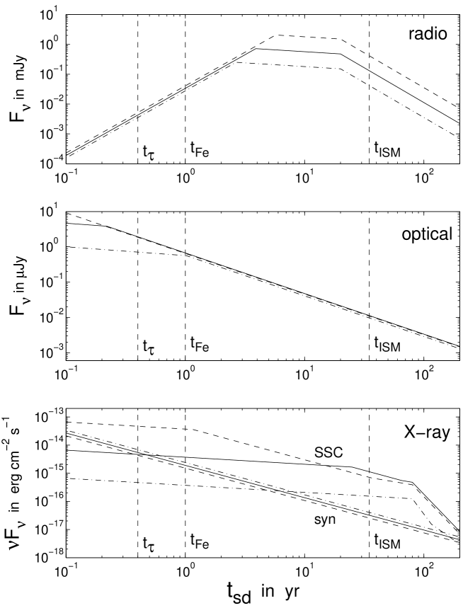
Figure 1: The flux density, $F_{\nu}$, of the plerion emission at the time of the GRB (i.e. a time $t_{\rm sd}$ after the supernova event), as a function of $t_{\rm sd}$. The three panels show the flux density in the radio, optical and X-ray bands ($\nu=5\times 10^{9},\,5\times 10^{14},\,10^{18}\;{\rm Hz}$, respectively). For the radio and optical we show $F_{\nu}$ of the synchrotron emission, and for the X-ray we show $\nu F_{\nu}$ for both the synchrotron and SSC components. The dashed, solid and dot-dashed lines represent $\log_{10}(\gamma_{w})=4,\,4.5$ and $5$, respectively. Dashed lines are shown at $t_{\tau}$ (below which the Thomson optical depth is larger than unity), $t_{\rm Fe}$ (below which iron line features can appear in the X-ray spectrum of the afterglow) and $t_{\rm ISM}$ (for which the effective density of the PWB is similar to that of a typical ISM, i.e. $1\;{\rm cm^{-3}}$.

The plerion emission at the radio, optical and X-ray bands is shown in Figure 1. For reference, we also show the times $t_{\tau}$ (below which the Thomson optical depth is larger than unity), $t_{\rm Fe}$ (below which iron line features can appear in the X-ray spectrum of the afterglow) and $t_{\rm ISM}$ (for which the effective density of the PWB is similar to that of a typical ISM, i.e. $1\;{\rm cm^{-3}}$). In the radio, the typical limiting flux for detection is $\sim 0.1\;{\rm mJy}$, and upper limits at this flux level, at a time $t<t_{\rm pl}$ after the GRB, would exclude $2\lesssim t_{\rm sd,0}\lesssim 20$ for $\gamma_{w}\lesssim 10^{5}$, while for $2\lesssim t_{\rm sd,0}\lesssim 65$ this would imply $\gamma_{w}\gtrsim 10^{4}$. Values of $t_{\rm sd}\lesssim 2\;{\rm yr}$ or $t_{\rm sd}\gtrsim 65\;{\rm yr}$ are hard to constrain with the radio.

Optical upper limits at the R-band at the level of $\sim 24-25$th magnitude ($F_{\nu}\lesssim 0.5{\rm\mu Jy}$) would imply $\gamma_{w}\gtrsim 10^{5}$ for $t_{\rm sd}<t_{\rm Fe}$, i.e. for afterglows with iron lines. More stringent upper limits, may provide more severe constraints. For example, an upper limit of $0.01\;{\rm\mu Jy}$ (i.e. R=28.6 which might be reached with HST) implies $t_{\rm sd}\gtrsim t_{\rm ISM}$.

In the X-ray, for $\gamma_{w}\lesssim 10^{4.5}$ the SSC emission dominates over the synchrotron emission for all $t_{\rm sd}\gtrsim t_{\tau}$, and for $\gamma_{w}=10^{5}$ it dominates for $t_{\rm sd}\gtrsim 7\;{\rm yr}$. The typical limiting flux for detection in the X-ray is a few $\times 10^{-14}\;{\rm erg\;cm^{-2}\;s^{-1}}$, and upper limits at this level may imply $\gamma_{w}\gtrsim 10^{4}$ for $t_{\rm sd}\lesssim t_{\rm Fe}$. For $t_{\rm sd}\gtrsim t_{\rm Fe}$, such upper limits cannot provide any useful constraints.

5 Effects on the Prompt GRB Emission

The prompt gamma-ray emission is believed to arise from internal shocks within the GRB outflow, due to variability in its Lorentz factor $\Gamma$ (Rees & Mészáros 1994; Sari & Piran 1997). In order for this process to be efficient, it needs to occur before the ejecta is significantly decelerated by the ambient medium. Therefore, the main effect that a plerionic environment may have on the prompt GRB stage is through inverse Compton scattering of the photons from the external plerion radiation field (which we shall refer to as external Compton, or EC).

The external (plerion) radiation field in the local rest frame of the shocked shells is $U^{\prime}_{ph,ext}=\Gamma^{2}U_{ph,ext}$ where $U_{ph,ext}$ is given by equation (54). The electrons radiatively cool by the combination of the synchrotron, SSC and EC processes the timescales for which are (in the comoving frame) $t^{\prime}_{\rm syn}\sim 6\pi m_{e}c/\sigma_{T}B^{\prime 2}\gamma$, $t^{\prime}_{SC}=t^{\prime}_{\rm syn}/Y$ and $t^{\prime}_{EC}=t^{\prime}_{\rm syn}/X$, where $Y$ is the Compton y-parameter and

$$X={U^{\prime}_{ph,ext}\over\epsilon_{B}e^{\prime}}=3.1\times 10^{-4}a^{1/2}f_{1/3}^{-2}\xi_{e,1/3}\epsilon_{be,1/3}^{-1/2}\epsilon_{bB,-3}^{1/2}\epsilon_{e}\epsilon_{B}^{-1}\beta_{b,-1}^{-2}t_{\rm sd,0}^{-3}E_{\rm rot,53}L_{52}^{-1}\Gamma_{2.5}^{8}t_{v,-2}^{2}\ ,$$ (69)

is the ratio of the energy density of the external radiation field and the magnetic field in the local rest frame of the shocked shells, which is also the ratio between the energies in the EC and synchrotron components. As can be seen from equation (69), $X\ll 1$ for typical parameters. In order to have $X\gtrsim 1$, we need $t_{\rm sd}\lesssim 1\;{\rm yr}$ and $\Gamma\gtrsim 10^{3}$. For an elongated PWB of the type described just before §4.1, with $f\sim R_{s}/R_{\rm eff}\sim 0.1$ and $\beta_{b}\approx 1$, $X$ is roughly the same.

The EC component is due to the scattering of external photons from the plerion radiation field by the electrons from the GRB ejecta. This scattering can be done either by hot (relativistic) electrons, or by cold (non-relativistic) electrons, the latter being either in cold shells or cold portions of colliding shells (in either regions before the shock, or at a distance larger than $\gamma_{c}\Delta^{\prime}$ behind the shock for $\gamma_{c}<1$).

For the colliding shells, we assume that Thomson optical depth, $\tau_{T}$, is smaller than 1. We provide detailed expressions for one representative plerion spectrum, the one given in equation (22), that is relevant for $t_{\rm sd}<t_{2}\sim 12\>{\rm yr}$ (see equation 35), which is of most interest. Similar expressions for the other plerion spectra can be readily derived in a similar manner. The plerion SSC emission in this regime has a peak for the $\nu F_{\nu}$ at $\nu_{bm}^{SC}\gtrsim 10^{20}\;{\rm Hz}$ for $t_{\rm sd}\lesssim 1\;{\rm yr}$, and will therefore be above the KN cutoff for both hot and cold electrons in the outflowing shells, and its contribution to the EC emission can be neglected. The resulting EC spectrum due to scattering by the hot electrons is

$${\nu F_{\nu}^{EC}\over\nu_{m}F_{\nu_{m}}}=X\times\left\{\matrix{(\nu_{sa}^{EC}/\nu^{EC}_{m})^{1/2}(\nu/\nu_{sa}^{EC})^{2}&\nu<\nu_{sa}^{EC}\cr&\cr(\nu/\nu^{EC}_{m})^{1/2}&\nu_{sa}^{EC}<\nu<\nu^{EC}_{m}\cr&\cr(\nu/\nu^{EC}_{m})^{1-s/2}&\nu^{EC}_{m}<\nu<\nu_{KN}^{EC}(\gamma_{M})}\right.\ .$$ (70)

where $\nu_{sa}^{EC}\equiv\Gamma^{2}\max(\gamma_{c}^{2},1)\nu_{bsa}$ and

$$\nu_{m}^{EC} = \Gamma^{2}\gamma_{m}^{2}\nu_{bm}\approx 1.9\times 10^{23}\eta_{2/3}^{5/2}\epsilon_{be,1/3}^{2}\epsilon_{bB,-3}^{1/2}\xi_{e,1/3}^{-2}E_{\rm rot,53}^{1/2}\gamma_{w,4.5}^{2}\beta_{b,-1}^{-3/2}t_{\rm sd,0}^{-3/2}\epsilon_{e}^{2}\Gamma_{2.5}^{2}\;{\rm Hz}\ ,$$

$$\nu_{KN,1}^{SC} = \nu_{KN,0}^{2}/\nu_{bm}\approx 3.0\times 10^{27}\eta_{2/3}^{-5/2}\epsilon_{be,1/3}^{-2}\epsilon_{bB,-3}^{-1/2}\xi_{e,1/3}^{2}E_{\rm rot,53}^{-1/2}\gamma_{w,4.5}^{-2}\beta_{b,-1}^{-3/2}t_{\rm sd,0}^{3/2}\;{\rm Hz}\ ,$$

$$\nu_{KN}^{SC}(\gamma_{M}) = \Gamma\gamma_{M}\nu_{KN,0}\approx 6.6\times 10^{27}(1+Y+X)^{-1/2}\epsilon_{e}^{1/4}\epsilon_{B}^{-1/4}L_{52}^{-1/4}\Gamma_{2.5}^{5/2}t_{v,-2}^{1/2}\;{\rm Hz}\ .$$ (71)

If $\nu_{KN,1}^{SC}<\nu_{KN}^{SC}(\gamma_{M})$ then we have $\nu F_{\nu}\propto\nu^{1/2-s}$ for $\nu_{KN,1}^{SC}<\nu<\nu_{KN}^{SC}(\gamma_{M})$. The peak of the $\nu F_{\nu}^{EC}$ spectrum, of the EC component from hot electrons is, is $\sim 10^{-10}(X/10^{-4})\;{\rm erg\,cm^{-2}\,s^{-1}}$ and is a factor of $X\sim 10^{-4}$ (for $t_{\rm sd}\sim 1\;{\rm yr}$) smaller than that of the synchrotron component, and therefore might be detected only for extreme parameters ($t_{\rm sd,0}\lesssim 1$, $\Gamma\gtrsim 10^{3}$).

For the scattering by cold electrons, the optical depth is approximately

$$\tau_{T}=\sigma_{t}n^{\prime}_{e}\Delta^{\prime}\approx 0.02\epsilon_{e}^{-1}L_{52}\Gamma_{2.5}^{-5}t_{v,-2}^{-1}\ ,$$ (72)

and the Compton y-parameter is $Y=\min(\tau_{T},1)\Gamma^{2}$. This implies that all frequencies of the plerion spectrum are shifted upwards by a factor of $\Gamma^{2}$, and the corresponding flux density, $F_{\nu}$, should be multiplied by $\min(\tau_{T},1)$. The only exception to this simple re-scaling is that the spectral slope below the upscattered self absorption frequency will be $F_{\nu}\propto\nu$, instead of the $\nu^{2}$ in the plerion spectrum. The peak of the $\nu F_{\nu}^{EC}$ spectrum will be at

$$\Gamma^{2}\nu_{bm}\approx 5.1\times 10^{18}\,(1+z)^{-1}\eta_{2/3}^{5/2}\epsilon_{be,1/3}^{2}\epsilon_{bB,-3}^{1/2}\xi_{e,1/3}^{-2}E_{\rm rot,53}^{1/2}\gamma_{w,4.5}^{2}\beta_{b,-1}^{-3/2}t_{\rm sd,0}^{-3/2}\;{\rm Hz}\ ,$$ (73)

which is typically at the hard X-ray or soft gamma-ray for $t_{\rm sd}\lesssim 1\;{\rm yr}$. However, the peak of $\nu F_{\nu}^{EC}$ for this component is a factor of $Y\leq\Gamma^{2}\sim 10^{5}$ larger than $\nu_{bm}F_{\nu_{bm}}\lesssim 10^{-14}\;{\rm erg\,cm^{-2}\,s^{-1}}$ and is therefore $\lesssim 10^{-9}\;{\rm erg\,cm^{-2}\,s^{-1}}$, and will typically hide below the standard GRB emission.

Another possible effect of the plerion radiation field is that photons with energy $\gtrsim 1\,t_{\rm sd,0}^{2}\;{\rm GeV}$ cannot escape the emission region due to a large opacity to pair production ($\tau_{\gamma\gamma}>1$). Therefore, all the components of the prompt GRB emission, including synchrotron, SSC and EC, will have an upper cutoff at this photon energy.

Finally, we consider the effect of the Compton drag due to the plerion radiation field on the GRB outflow. The effect of Compton drag in GRBs was considered in the context of the collapsar model, where the radiation comes from the walls of a funnel along the rotational axis of the progenitor star (Ghisellini et al. 2000; Lazzati et al. 2000). The rate of energy loss of a shell of initial Lorentz factor $\Gamma_{0}$ rest mass $M$ and solid angle $\Omega_{j}$, is given by

$${dE\over dt}={d\Gamma\over dt}Mc^{2}=-\Omega_{j}R^{2}c\Gamma^{2}U_{ph}\min(\tau_{T},1)$$ (74)

where $t\approx R/c$ is the lab frame time, $\tau_{T}=(R/R_{\tau})^{-2}$ is the Thomson optical depth of the shell, $R_{\tau}$ is the radius where this optical depth drops below unity. We render Eq. 74 dimensionless by introducing $\tilde{R}\equiv R/R_{\tau}=\tau_{T}^{-1/2}$,

$${d(1/\Gamma)\over d\tilde{R}}=A\min(\tilde{R}^{2},1)\quad,\quad A\equiv{\Omega U_{ph}R_{\tau}^{3}\over Mc^{2}}$$ (75)

This gives

$${\Gamma(\tilde{R})\over\Gamma_{0}}=\left\{\matrix{(1+A\Gamma_{0}\tilde{R}^{3}/3)^{-1}&\tilde{R}<1\ \ \cr&\cr\left[1+A\Gamma_{0}(\tilde{R}-2/3)\right]^{-1}&\tilde{R}>1\ \ }\right.\ ,$$ (76)

where

$$R_{\tau} = 3.3\times 10^{12}\,\epsilon_{\gamma}^{-1/2}L_{52}^{1/2}\Gamma_{2.5}^{-1/2}t_{v,-2}^{1/2}\;{\rm cm}\ ,$$

$$A = 1.6\times 10^{-8}a\,f_{1/3}^{-2}\epsilon_{\gamma}^{-1/2}\xi_{e,1/3}E_{\rm rot,53}\beta_{b,-1}^{-2}t_{\rm sd,0}^{-3}L_{52}^{1/2}\Gamma_{2.5}^{-1/2}t_{v,-2}^{1/2}\ ,$$ (77)

where $\epsilon_{\gamma}$ is the fraction of the kinetic luminosity of the GRB outflow that is converted into the gamma-ray emission. As can be seen from Eqs. (76) and (77), $A\Gamma_{0}\ll 1$ and therefore $\Gamma(R_{\tau})\cong\Gamma_{0}$, while for $R\gg R_{\tau}$ the fractional change in $\Gamma$ is given by $A\Gamma_{0}\tilde{R}$. If the radius, $R_{\rm cd}$, at which deceleration due to Compton drag becomes significant, is larger than the deceleration radius, $R_{\rm dec}\approx fR_{b}$, due to the sweeping up ofthe PWB material, then the deceleration due to Compton drag is at most comparable (and never dominant) to the deceleration due to the ambient medium, for $k\leq 1$. Therefore, Compton drag will have a significant effect on the decelleration only if $R_{\rm cd}<R_{\rm dec}$, which for our fiducial values may be expressed as $t_{\rm sd}<0.3f^{1/2}\;$yr. For such low values of $t_{\rm sd}$ the SNR shell is still optically thick to Compton scattering ($t_{\rm sd}<t_{\tau}$), so that we do not expect to see the GRB or afterglow emission. We conclude that the deceleration of the GRB ejecta due to Compton drag is negligible for relevant values of $t_{\rm sd}$.

6 Effects on the Afterglow Emission

At a time $t_{\rm sd}$ after the supernova event, the SMNS collapses and triggers the GRB explosion, sending a fireball and relativistic blast wave into the PWB. When the GRB ejecta has swept up enough of the outlying material, it is decelerated, and it drives a strong relativistic shock into the external medium, that is responsible for the afterglow (AG) emission.

In this section we study the observational consequences of the plerionic environment inside the PWB, that are different from the standard “cold”, weakly magnetized proton-electron external medium. One of the advantages of having the PWB as the environment for the GRB afterglow is that it naturally yields high values of $\epsilon_{e}$ and $\epsilon_{B}$ (the fraction of the internal energy in the electrons and in the magnetic field, respectively) behind the AG shock (KG). High values of $\epsilon_{e}$ are expected from the fact that relativistic pulsar-type winds are likely dominated by an electron-positron component, whereas significant values of $\epsilon_{B}$ should naturally occur if the winds are characterized by a high magnetization parameter. We expect $\epsilon_{B}\sim\epsilon_{bB}$, and use the same fiducial value for these two parameters. The electrons in the PWB are typically colder than the protons by the time the afterglow shock arrives, and most of the energy is in the internal energy of the hot protons. This might suggest that $\epsilon_{e}$ can be slightly smaller than $\epsilon_{be}$ and motivates us to use $\epsilon_{e}=\epsilon_{e,-1}/10$ for our fiducial values.

The values of the physical quantities behind the AG shock can be determined from the appropriate generalizations of the hydrodynamic conditions used in the case of a “cold” medium taking into account the fact that the preshock gas is now “hot” and should be well described by a relativistic equation of state, $p=e/3=w/4$, where $w$ is the enthalpy density and $p$ is the particle pressure. In the following we largely follow the analysis of KG . The deceleration of the AG shock is determined by the total enthalpy of the external medium, $w_{tot}$, which includes contributions from the particles and the magnetic field enthalpy, $B^{2}/4\pi$, where the latter contribution is negligible for our choice of parameters ($\epsilon_{B}\ll 1$). This make it convenient to define an “equivalent” hydrogen number density $n_{\rm H,equiv}\equiv w_{\rm tot}/m_{p}c^{2}\approx w/m_{p}c^{2}=(4/3)e/m_{p}c^{2}$, in analogy with the traditional parameterization of the external medium enthalpy density, $w=n_{\rm H}m_{p}c^{2}$, that is relevant for a standard ISM or stellar-wind environment.

In general both the energy and the electron number density may be function of the distance $r$ from the center of the PWB and can be parametrized as

$$e(r) = A_{e}r^{-k_{*}}\quad;\quad A_{e}=\frac{(3-k_{*})\eta E_{\rm rot}}{4\pi R_{b}^{3-k}}\ ,$$ (78)

$$n_{e}(r) = A_{n}r^{-k}\quad;\quad A_{n}=\frac{(3-k)N_{e}}{4\pi R_{b}^{3-k}}\ ,$$ (79)

where $N_{e}=\dot{N}_{e}t_{\rm sd}$ is the total number of the electrons in the PWB and $\dot{N}_{e}$ is given in Eq. 10. When a large fraction of the energy density in the PWB goes to the proton component we have $\eta\sim 1$ and we can expect both $n_{\rm H,equiv}$ and $n_{e}$ to have a similar radial dependence, i.e. $k=k_{*}$. The expected values of $k$ typically ranges between $k=0$, similar the the ISM, and $k=1$, that is intermediate between an ISM and a stellar wind (KG). For an elongated PWB, things can get much more complicated, since $e$ and $n_{e}$ can depend not only on $r$ but also on the angle $\theta$ from the polar axis. However, if the $\theta$ dependence within the opening angle of the GRB jet is small, and the dependence on $r$ may be reasonably approximated by a power law, then our formalism still holds for $k\approx 0$, with the usual substitution of $\beta_{b}=3R_{\rm eff}/2ct_{\rm sd}$ (see the beginning of §4). For $k>0$ we also need to change the normalization in equation (78) and (79) accordingly.

The expressions for the radius $R_{AG}$ and the Lorentz factor $\Gamma_{AG}$ of the shocked AG material can be derived using energy conservation

$$E_{\rm iso}=\Gamma^{2}_{AG}\int^{R_{AG}}_{R_{S}}n_{\rm H,equiv}m_{p}c^{2}4\pi r^{2}dr\,,$$ (80)

where $E_{\rm iso}$ is the isotropic equivalent energy of the AG shock, and using the relation

$$t\sim\frac{R_{AG}}{4c\Gamma_{AG}^{2}}\ ,$$ (81)

where $t$ is the observed time. We obtain

$$R_{AG}=\left[\frac{3E_{\rm iso}ctR_{b}^{3-k}}{\eta\,E_{\rm rot}}\right]^{1/(4-k)}$$ (82)

$$\Gamma_{AG}=\sqrt{\frac{R_{AG}}{4ct}}\propto t^{(k-3)\over 2(4-k)}\propto\left\{\matrix{t^{-3/8}&\quad k=0\cr&\cr t^{-1/3}&\quad k=1}\right.\ .$$ (83)

The postshock energy and particle density (in the shock comoving frame) are given by

$$e^{\prime}=4\Gamma^{2}_{AG}w\quad,\quad n_{e}^{\prime}=4\Gamma_{AG}n_{e}$$ (84)

The electron distribution is assumed to be similar to that of internal shocks, $N(\gamma)\propto\gamma^{-p}$ for $\gamma_{m}<\gamma<\gamma_{M}$, and we use $p=2.5$ to obtain the numerical values.

As mentioned in §4.4, the plerion radiation field is roughly homogeneous and isotropic within the the radius $fR_{b}$ where the plerion emission takes place. At $r\lesssim fR_{b}$ the external (plerion) photon energy density, $U_{ph,ext}$, is given by equation (54), and we may use the relation $U^{\prime}_{ph,ext}=\Gamma_{AG}^{2}U_{ph,ext}$ (that is valid for an isotropic radiation field) to obtain

$$X={U^{\prime}_{ph,ext}\over\epsilon_{B}e^{\prime}}\approx\left\{\matrix{2.1\,a^{1/2}\,f_{1/3}^{-2}\eta_{2/3}^{-1}\epsilon_{be,1/3}^{-1/2}\epsilon_{bB,-3}^{1/2}\epsilon_{B,-3}^{-1}\xi_{e,1/3}\beta_{b,-1}&k=0\cr&\cr 1.8\,a^{1/2}\,f_{1/3}^{-2}\eta_{2/3}^{-4/3}\epsilon_{be,1/3}^{-1/2}\epsilon_{bB,-3}^{1/2}\epsilon_{B,-3}^{-1}\xi_{e,1/3}E_{\rm rot,53}^{-1/3}\beta_{b,-1}^{2/3}t_{sd,1.5}^{-1/3}E_{\rm iso,53}^{1/3}t_{\rm days}^{1/3}&k=1}\right.\ ,$$ (85)

where $t_{sd,1.5}=t_{sd}/10^{1.5}$. For $t_{\rm sd}>t_{3}\sim 65\;{\rm yr}$ the PWB is slow cooling, and $f=1$, so that $R_{AG}<fR_{b}$ throughout the afterglow. For $t_{\rm sd}<t_{3}$ the plerion emission is radiated within a shell of width $R_{b}-R_{s}$ times the ratio, $(t_{\rm sd}/t_{3})^{2}$, of the cooling time of electrons with $\gamma_{bm}$, and the dynamical time $t_{\rm sd}$. This implies that generally, $f=\min\{1,(R_{s}/R_{b})[1-(t_{\rm sd}/t_{3})^{2}]+(t_{\rm sd}/t_{3})^{2}\}$. For $t_{\rm sd}<t_{3}$ we have $f<1$ and therefore $R_{AG}<fR_{b}$ only at sufficiently early times after the GRB. For $t_{\rm sd}\ll t_{3}$, the radiation is emitted within a thin shell behind the wind termination shock, at $R_{s}$, and $f\approx R_{s}/R_{b}$. In this case $R_{AG}>fR_{b}$ throughout the afterglow. We study the implications in the following.

At $r>fR_{b}$, the plerion radiation field is no longer isotropic or homogeneous, and we model the plerion radiation field as resulting from emission by a uniformly bright sphere with a radius $fR_{b}$, and obtain

$$U_{ph}={\xi_{e}L_{w}\over 2\pi cfR_{b}^{2}}(1-\mu)\approx{\xi_{e}L_{w}\over 4\pi c\,r^{2}}\quad,\quad U^{\prime}_{ph}={\xi_{e}L_{w}\over 2\pi cfR_{b}^{2}}{\Gamma_{AG}^{2}\over 3\beta}[(1-\beta\mu)^{3}-(1-\beta)^{3}]\ ,$$ (86)

where $\mu\equiv[1-(fR_{b}/r)^{2}]^{1/2}$ and $\beta=(1-\Gamma_{AG}^{-2})^{1/2}$. The ratio of the photon energy in the local and the observer frames is now

$${U^{\prime}_{ph}\over U_{ph}}={\Gamma_{AG}^{2}\left[(1-\beta\mu)^{3}-(1-\beta)^{3}\right]\over 3\beta(1-\mu)}\approx\left\{\matrix{\Gamma_{AG}^{2}(1-\mu)^{2}/3\approx(fR_{b}/r)^{4}\Gamma_{AG}^{2}/12&r\ll\Gamma_{AG}fR_{b}\cr&\cr(1-\beta)/(1+\beta)\approx 1/4\Gamma_{AG}^{2}&r\gg\Gamma_{AG}fR_{b}}\right.\ .$$ (87)

During the early afterglow, $R_{AG}$ is relatively small and $\Gamma_{AG}\gg 1$, so that $R_{AG}\ll\Gamma_{AG}fR_{b}$, and the first limit of equation (87) is applicable, implying

$$X_{1}\approx\left\{\matrix{0.26\,a^{-1/2}f_{1/3}^{4}\eta_{2/3}^{1/2}\epsilon_{be,1/3}^{-1/2}\epsilon_{bB,-3}^{1/2}\epsilon_{B,-3}^{-1}\xi_{e,1/3}E_{\rm rot,53}^{3/2}\beta_{b,-1}^{5/2}t_{sd,1.5}^{3/2}E_{\rm iso,53}^{-3/2}t_{\rm days}^{-3/2}&k=0\cr&\cr 0.93\,a^{-1/2}f_{1/3}^{4}\eta_{2/3}^{2/3}\epsilon_{be,1/3}^{-1/2}\epsilon_{bB,-3}^{1/2}\epsilon_{B,-3}^{-1}\xi_{e,1/3}E_{\rm rot,53}^{5/3}\beta_{b,-1}^{8/3}t_{sd,1.5}^{5/3}E_{\rm iso,53}^{-5/3}t_{\rm days}^{-5/3}&k=1}\right.\ .$$ (88)

During the course of the afterglow its radius increases while its Lorentz factor decreases, so that eventually $R_{AG}$ becomes larger than $\Gamma_{AG}fR_{b}$, and the second limit of equation (87) becomes relevant, implying

$$X_{2}\approx\left\{\matrix{1.3\times 10^{-4}\,a^{-1/2}\epsilon_{be,1/3}^{-1/2}\epsilon_{bB,-3}^{1/2}\epsilon_{B,-3}^{-1}\xi_{e,1/3}E_{\rm rot,53}t_{sd,1.5}^{3/2}E_{\rm iso,53}^{-1}t_{\rm days}&k=0\cr&\cr 2.0\times 10^{-4}\,a^{-1/2}\epsilon_{be,1/3}^{-1/2}\epsilon_{bB,-3}^{1/2}\epsilon_{B,-3}^{-1}\xi_{e,1/3}E_{\rm rot,53}t_{sd,1.5}^{3/2}E_{\rm iso,53}^{-1}t_{\rm days}&k=1}\right.\ ,$$ (89)

as long as the afterglow shock is still relativistic. One can combine the two limits and use $X=\max(X_{1},X_{2})$. However, since the region where these asymptotic expressions for $X$ are not a very good approximation may play an important role, we use equation (86) rather than equations (88) and (89) for all our calculations.

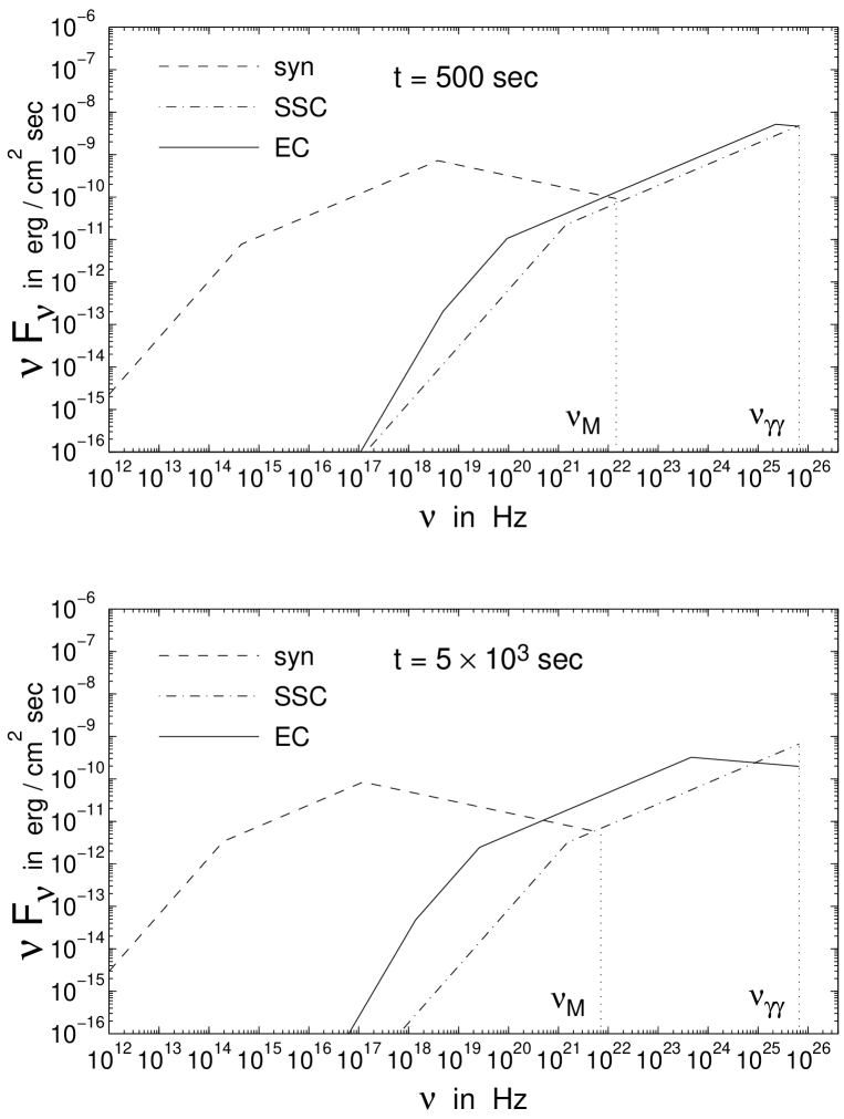
Figure 2: The afterglow $\nu F_{\nu}$ spectrum at $t=500\;{\rm s}$ (upper panel) and $5\times 10^{3}\;{\rm s}$ (lower panel) after the GRB, for our fiducial parameters, and for $t_{\rm sd}=20\;{\rm yr}$, $E_{\rm rot,53}=0.5$, $z=1$, $R_{s}/R_{b}=0.1$. Dotted vertical lines indicate $\nu_{M}$ where the upper cutoff for the synchrotron emission is located, and $\nu_{\gamma\gamma}$ where the upper cutoff of the SSC and EC (due to pair opacity) is located.

It is also worth to note that the average shift in frequency of the photons between the observer frame and local and rest frame is $\langle\nu^{\prime}/\nu\rangle=\Gamma_{AG}[1-\beta(1+\mu)/2]\approx[1+\Gamma_{AG}^{2}(1-\mu)^{2}]/2\Gamma_{AG}$, and varies between $\Gamma_{AG}/2$ and $1/2\Gamma_{AG}$. This should be compared to the usual factor of $\Gamma_{AG}$ for an isotropic (plerion) radiation field, and implies lower typical EC frequencies, by a factor of $[1-\beta(1+\mu)/2]$. For simplicity we do not include this factor in the expressions for the EC frequencies, but we do take it into account in Figure 2, and when deriving constraints on the model parameters.

The electron cooling time is $t_{\rm syn}/(1+Y+X)$ where the Compton y-parameter may be obtained by solving the equation

$$Y\approx\tau_{T}a\gamma_{c}\gamma_{m}\approx{a\epsilon_{e}\over\epsilon_{B}(1+Y+X)}\ ,$$ (90)

which gives (Granot & Königl 2001):

$$Y\approx\left\{\matrix{\sqrt{a\epsilon_{e}/\epsilon_{B}}&1,X^{2}\ll a\epsilon_{e}/\epsilon_{B}\cr&\cr a\epsilon_{e}/\epsilon_{B}&X,\,a\epsilon_{e}/\epsilon_{B}\ll 1\cr&\cr a\epsilon_{e}/(\epsilon_{B}X)&a\epsilon_{e}/\epsilon_{B},\,1\ll X^{2}}\right.\ .$$ (91)

For our choice of parameters, $\epsilon_{B}\ll\epsilon_{e}$ and $a\epsilon_{e}/\epsilon_{B}\gg 1$, so that either the first or the third limits of Eq. (91) are relevant. As the first limit is more often applicable, we use the parameterization $(1+Y+X)\equiv\bar{X}(a\epsilon_{e}/\epsilon_{B})^{1/2}$, so that the numerical coefficients and explicit dependence on the parameters of the break frequencies (that depend on the electron cooling time), would be relevant for $X^{2}\ll a\epsilon_{e}/\epsilon_{B}$, where $\bar{X}\approx 1$. In the limit $X^{2}\gg a\epsilon_{e}/\epsilon_{B}$, the numerical coefficients and parameter dependences change because of the dependence on $\bar{X}\approx X/(a\epsilon_{e}/\epsilon_{B})^{1/2}$, which is no longer close to 1 in this limit.

6.1 The Synchrotron Emission

In the standard case of a uniform ambient medium, one can express the break frequencies and the peak flux in terms of the shock energy $E$, the ambient density $n_{\rm H}$, the observed time $t$, as well as $\epsilon_{e}$, $\epsilon_{B}$, and the distance to the source (Sari, Piran & Narayan 1998). This is thanks to the fact that for a ’standard’ external medium that is composed of equal numbers of protons and electrons, so that both the shock dynamics (that is determined by $w=n_{\rm H}m_{p}c^{2}$) and the external number density of electrons (that enter the expressions for the flux normalization and self absorption frequency), are determined by a single parameter, $n_{\rm H}$. In the case of a shock propagating inside a PWB, the dynamics of the AG shock are determined by $w=n_{\rm H,equiv}m_{p}c^{2}\approx\eta\gamma_{w}n_{p}m_{p}c^{2}$ that is dominated by the internal energy of the hot protons, while the number density of electrons is different, and dominated by the electron-positron pairs. We find

$$n_{\rm H,equiv} = {\eta E_{\rm rot}\over\pi R_{b}^{3}m_{p}c^{2}}\approx 1.8\,\eta_{2/3}E_{\rm rot,53}\beta_{b,-1}^{-3}t_{\rm sd,1.5}^{-3}\ ,$$

$${n_{e}\over n_{\rm H,equiv}} = {3\xi_{e}m_{p}\over 4\eta_{e}\gamma_{w}m_{e}}\approx 0.022\,\eta_{2/3}^{-1}\xi_{e,1/3}\gamma_{w,4.5}^{-1}\ .$$ (92)

For an elongated PWB we can make the usual substitution $\beta_{b}=3R_{\rm eff}/2ct_{\rm sd}$, to obtain the relevant expressions (see discussion just before §4.1).

The self absorption frequency is typically $\nu_{sa}<\min(\nu_{c},\nu_{m})$, and is calculated using equation (30) for fast cooling and equation (34) for slow cooling, solving for $\tau_{\nu}^{\prime}=\alpha^{\prime}R_{AG}/\Gamma_{AG}=1$ for $\nu^{\prime}_{sa}$ and then $\nu_{sa}=\Gamma_{AG}\nu^{\prime}_{sa}$. The transition time from fast to slow cooling, $t_{0}$, is obtained by equating $\gamma_{c}$ and $\gamma_{m}$. For $k=0$ we get

$$\nu_{c} \approx 2.1\times 10^{14}\,(1+z)^{-1/2}a^{-1}\bar{X}^{-2}\eta_{2/3}^{-1}\epsilon_{e,-1}^{-1}\epsilon_{B,-3}^{-1/2}E_{\rm rot,53}^{-1}\beta_{b,-1}^{3}t_{\rm sd,1.5}^{3}E_{\rm iso,53}^{-1/2}t_{\rm days}^{-1/2}\;{\rm Hz}\ ,$$

$$\nu_{m} \approx 1.2\times 10^{15}\,(1+z)^{1/2}\eta_{2/3}^{2}\xi_{e,1/3}^{-2}\epsilon_{e,-1}^{2}\epsilon_{B,-3}^{1/2}\gamma_{w,4.5}^{2}E_{\rm iso,53}^{1/2}t_{\rm days}^{-3/2}\;{\rm Hz}\ ,$$

$$\nu_{M} \approx 5.2\times 10^{21}\,(1+z)^{-5/8}a^{-1/2}\bar{X}^{-1}\eta_{2/3}^{-1/8}\epsilon_{e,-1}^{-1/2}\epsilon_{B,-3}^{1/2}E_{\rm rot,53}^{-1/8}\beta_{b,-1}^{3/8}t_{\rm sd,1.5}^{3/8}E_{\rm iso,53}^{1/8}t_{\rm days}^{-3/8}\;{\rm Hz}\ ,$$

$$\nu_{sa1} \approx 1.0\times 10^{8}\,(1+z)^{-1/2}\bar{X}\eta_{2/3}^{1/2}\xi_{e,1/3}^{3/5}\epsilon_{e,-1}^{1/2}\epsilon_{B,-3}^{7/10}E_{\rm rot,53}^{11/10}\gamma_{w,4.5}^{-3/5}\beta_{b,-1}^{-3.3}t_{\rm sd,1.5}^{-3.3}E_{\rm iso,53}^{7/10}t_{\rm days}^{-1/2}\;{\rm Hz}\ ,$$

$$\nu_{sa2} \approx 2.6\times 10^{7}\,(1+z)^{-1}\eta_{2/3}^{-1}\xi_{e,1/3}^{8/5}\epsilon_{e,-1}^{-1}\epsilon_{B,-3}^{1/5}E_{\rm rot,53}^{3/5}\gamma_{w,4.5}^{-8/5}\beta_{b,-1}^{-9/5}t_{\rm sd,1.5}^{-9/5}E_{\rm iso,53}^{1/5}\;{\rm Hz}\ ,$$ (93)

$$F_{\nu,{\rm max}} \approx 0.61\,(1+z)\eta_{2/3}^{-1/2}\xi_{e,1/3}\epsilon_{B,-3}^{1/2}E_{\rm rot,53}^{1/2}\gamma_{w,4.5}^{-1}\beta_{b,-1}^{-3/2}t_{\rm sd,1.5}^{-3/2}E_{\rm iso,53}d_{L28}^{-2}{\rm mJy}\ ,$$

$$t_{0} \approx 5.7\,(1+z)\bar{X}^{2}\eta_{2/3}^{3}\xi_{e,1/3}^{-2}\epsilon_{e,-1}^{3}\epsilon_{B,-3}E_{\rm rot,53}\gamma_{w,4.5}^{2}\beta_{b,-1}^{-3}t_{\rm sd,1.5}^{-3}E_{\rm iso,53}\;{\rm days}\ ,$$

where $\nu_{sa1}$ is for fast cooling and $\nu_{sa2}$ is for slow cooling. For k=1 we get

$$\nu_{c} \approx 7.0\times 10^{13}\,(1+z)^{-5/6}a^{-1}\bar{X}^{-2}\eta_{2/3}^{-4/3}\epsilon_{e,-1}^{-1}\epsilon_{B,-3}^{-1/2}E_{\rm rot,53}^{-4/3}\beta_{b,-1}^{8/3}t_{\rm sd,1.5}^{8/3}E_{\rm iso,53}^{-1/6}t_{\rm days}^{-1/6}\;{\rm Hz}\ ,$$

$$\nu_{m} \approx 9.9\times 10^{14}\,(1+z)^{1/2}\eta_{2/3}^{2}\xi_{e,1/3}^{-2}\epsilon_{e,-1}^{2}\epsilon_{B,-3}^{1/2}\gamma_{w,4.5}^{2}E_{\rm iso,53}^{1/2}t_{\rm days}^{-3/2}\;{\rm Hz}\ ,$$

$$\nu_{M} \approx 4.2\times 10^{21}\,(1+z)^{-2/3}a^{-1/2}\bar{X}^{-1}\eta_{2/3}^{-1/6}\epsilon_{e,-1}^{-1/2}\epsilon_{B,-3}^{1/2}E_{\rm rot,53}^{-1/6}\beta_{b,-1}^{1/3}t_{\rm sd,1.5}^{1/3}E_{\rm iso,53}^{1/6}t_{\rm days}^{-1/3}\;{\rm Hz}\ ,$$

$$\nu_{sa1} \approx 3.3\times 10^{8}\,(1+z)^{-2/15}\bar{X}\eta_{2/3}^{13/15}\xi_{e,1/3}^{3/5}\epsilon_{e,-1}^{1/2}\epsilon_{B,-3}^{7/10}E_{\rm rot,53}^{22/15}\gamma_{w,4.5}^{-3/5}\beta_{b,-1}^{-44/15}t_{\rm sd,1.5}^{-44/15}E_{\rm iso,53}^{1/3}t_{\rm days}^{-13/15}\;{\rm Hz}\ ,$$

$$\nu_{sa2} \approx 5.2\times 10^{7}\,(1+z)^{-4/5}\eta_{2/3}^{-4/5}\xi_{e,1/3}^{8/5}\epsilon_{e,-1}^{-1}\epsilon_{B,-3}^{1/5}E_{\rm rot,53}^{4/5}\gamma_{w,4.5}^{-8/5}\beta_{b,-1}^{-8/5}t_{\rm sd,1.5}^{-8/5}t_{\rm days}^{-1/5}\;{\rm Hz}\ ,$$ (94)

$$F_{\nu,{\rm max}} \approx 1.2\,(1+z)^{7/6}\eta_{2/3}^{-1/3}\xi_{e,1/3}\epsilon_{B,-3}^{1/2}E^{2/3}_{\rm rot,53}\gamma_{w,4.5}^{-1}\beta_{b,-1}^{-4/3}t_{\rm sd,1.5}^{-4/3}E_{\rm iso,53}^{5/6}t_{\rm days}^{-1/6}d_{L28}^{-2}\;{\rm mJy}\ ,$$

$$t_{0} \approx 7.3\,(1+z)\bar{X}^{3/2}\eta_{2/3}^{5/2}\xi_{e,1/3}^{-3/2}\epsilon_{e,-1}^{9/4}\epsilon_{B,-3}^{3/4}E_{\rm rot,53}\gamma_{w,4.5}^{3/2}\beta_{b,-1}^{-2}t_{\rm sd,1.5}^{-2}E_{\rm iso,53}^{1/2}\;{\rm days}\ ,$$

We note that in order for $\nu_{sa}$ not to exceed a few GHz, as typically implied by observations, we need $t_{\rm sd}\gtrsim 10\;{\rm yr}$. This also gives more reasonable values for the transition time from fast to slow cooling, $t_{0}$, and for $F_{\nu,{\rm max}}$. For $k=0$ the effective mass density of the PWB, becomes similar to that of a typical ISM, $n_{\rm H,equiv}=1\;{\rm cm^{-3}}$, for

$$t_{\rm ISM}=38\,\eta_{2/3}^{1/3}E_{\rm rot,53}^{1/3}\beta_{b,-1}^{-1}\;{\rm yr}\ ,$$ (95)

while the electron number density reaches the same value for a smaller $t_{\rm sd}=10.7\,\eta_{2/3}^{1/6}\xi_{e,1/3}^{1/6}\gamma_{w,4.5}^{-1/6}\beta_{b,-1}^{-1}\;{\rm yr}$. For $t_{\rm sd}\sim t_{\rm ISM}$ the afterglow emission is close to that of the ’standard’ model, where the external medium is the ISM or a stellar wind, which has been extensively and successfully fitted to afterglow observations.

In order to explain the X-ray lines, we need $t_{\rm sd}\lesssim t_{\rm Fe}\sim 1\;{\rm yr}$. This implies that the radio will typically be below the self absorption frequency, and hence the radio emission from the afterglow would not be detectable. On top of this, the jet break time is given by substituting $n_{\rm H,equiv}$ in place of the external density for a ’standard’ external medium (Sari, Piran & Halpern 1999),

$$t_{j}=1.1\,\left({1+z\over 2}\right)\left(E_{iso,53}\over n_{H,equiv,0}\right)^{1/3}\theta_{j,-1}^{8/3}\;{\rm days}$$ (96)

$$\quad\quad\quad\quad\quad\ =0.70\,\left({1+z\over 2}\right)\left({E_{\rm iso,53}\over\eta_{2/3}E_{\rm rot,53}}\right)^{1/3}\beta_{b,-1}t_{\rm sd,0}\theta_{j,-1}^{8/3}\;{\rm hr}\ ,$$

and is very low for $\theta_{j,-1}=\theta_{j}/0.1\sim 1$. If we want to explain the observed values of $t_{j}\sim 1\;{\rm day}$ that are typically observed as resulting from a larger $\theta_{j}$ ($\sim 0.4$) then this would imply that the time of transition to a non-relativistic flow should be $t_{\rm NR}\sim\theta_{j}^{-2}t_{j}\sim 7\,t_{j}\sim 7\,{\rm days}$, and in general,

$$t_{\rm NR}\sim{1\over c}\left({E\over n_{H,equiv}m_{p}c^{2}}\right)^{1/3}\approx 18\,\left({1+z\over 2}\right)\left({E_{51}\over\eta_{2/3}E_{\rm rot,53}}\right)^{1/3}\beta_{b,-1}t_{\rm sd,0}\;{\rm days}\ ,$$ (97)

where $E=10^{51}E_{51}\;{\rm ergs}$ is the true energy of the afterglow, and we have dropped factors of order unity. Finally, for $t_{\rm sd}\lesssim t_{\rm Fe}\sim 1\;{\rm yr}$, the transition time from fast to slow cooling is very large, and fast cooling is expected during all the afterglow.

For $t<t_{0}$, in the fast cooling regime, the synchrotron flux density, $F_{\nu}$, is given by:

$$F_{\nu}=F_{\nu,{\rm max}}\times\left\{\matrix{(\nu_{sa}/\nu_{c})^{1/3}(\nu/\nu_{sa})^{2}&\ \ \nu<\nu_{sa}\cr&\cr(\nu/\nu_{c})^{1/3}&\ \ \nu_{sa}<\nu<\nu_{c}\cr&\cr(\nu/\nu_{c})^{-1/2}&\nu_{c}<\nu<\nu_{m}\cr&\cr(\nu_{m}/\nu_{c})^{-1/2}(\nu/\nu_{m})^{-p/2}&\nu_{m}<\nu<\nu_{M}}\right.\ ,$$ (98)

For $t>t_{0}$ we are in the slow cooling regime, in this case the spectrum peaks at $\nu_{m}$ and again consists of four power law segments:

$$F_{\nu}=F_{\nu,{\rm max}}\times\left\{\matrix{(\nu_{sa}/\nu_{m})^{1/3}(\nu/\nu_{sa})^{2}&\ \ \nu<\nu_{sa}\cr&\cr(\nu/\nu_{m})^{1/3}&\ \ \nu_{sa}<\nu<\nu_{m}\cr&\cr(\nu/\nu_{m})^{(1-p)/2}&\nu_{m}<\nu<\nu_{c}\cr&\cr(\nu_{c}/\nu_{m})^{(1-p)/2}(\nu/\nu_{c})^{-p/2}&\nu_{c}<\nu<\nu_{M}}\right.\ .$$ (99)

6.2 The SSC Emission

The SSC emission is calculated similarly to §4.2 and §4.3. The fast cooling spectrum is given by

$${\nu F_{\nu}^{SC}\over\nu_{m}F_{\nu_{m}}}=Y\times\left\{\matrix{(\nu^{SC}_{c}/\nu^{SC}_{m})^{1/2}(\nu^{SC}_{sa}/\nu^{SC}_{c})^{4/3}(\nu/\nu^{SC}_{sa})^{2}&\ \ \nu<\nu^{SC}_{sa}\cr&\cr(\nu^{SC}_{c}/\nu^{SC}_{m})^{1/2}(\nu/\nu^{SC}_{c})^{4/3}&\nu^{SC}_{sa}<\nu<\nu^{SC}_{c}\cr&\cr(\nu/\nu^{SC}_{m})^{1/2}&\nu^{SC}_{c}<\nu<\nu^{SC}_{m}\cr&\cr(\nu/\nu^{SC}_{m})^{1-p/2}&\nu^{SC}_{m}<\nu<\nu_{KN,1}^{SC}\cr&\cr(\nu_{KN,1}^{SC}/\nu^{SC}_{m})^{1-p/2}(\nu/\nu_{KN,1}^{SC})^{1/2-p}&\nu_{KN,1}^{SC}<\nu<\nu_{KN}^{SC}(\gamma_{M})}\right.\ ,$$ (100)

where

$$\nu_{m}F_{\nu_{m}}=3.1\times 10^{-12}\,(1+z)\bar{X}^{-1}\epsilon_{e,-1}^{1/2}\epsilon_{B,-3}^{1/2}E_{\rm iso,53}t_{\rm days}^{-1}d_{L28}^{-2}{\rm erg\,\,cm^{-2}\,s^{-1}}\ ,$$ (101)

and for $k=0$ we have

$$\nu^{SC}_{sa} \approx \gamma_{c}^{2}\nu_{sa1}\approx{3.9\times 10^{15}\over(1+z)^{3/4}}\,\bar{X}^{-1}\eta_{2/3}^{-3/4}\xi_{e,1/3}^{3/5}\epsilon_{e,-1}^{-1/2}\epsilon_{B,-3}^{-3/10}E_{\rm rot,53}^{-3/20}\gamma_{w,4.5}^{-3/5}\beta_{b,-1}^{9/20}t_{\rm sd,1.5}^{9/20}E_{\rm iso,53}^{-1/20}t_{\rm days}^{-1/4}\;{\rm Hz}\ ,$$

$$\nu^{SC}_{c} \approx \gamma_{c}^{2}\nu_{c}\approx{1.5\times 10^{22}\over(1+z)^{3/4}}\,a^{-2}\bar{X}^{-4}\eta_{2/3}^{-9/4}\epsilon_{e,-1}^{-2}\epsilon_{B,-3}^{-3/2}E_{\rm rot,53}^{-9/4}\beta_{b,-1}^{27/4}t_{\rm sd,1.5}^{27/4}E_{\rm iso,53}^{-5/4}t_{\rm days}^{-1/4}\;{\rm Hz}\ ,$$

$$\nu^{SC}_{m} \approx \gamma_{m}^{2}\nu_{m}\approx{5.1\times 10^{23}\over(1+z)^{-5/4}}\,\eta_{2/3}^{15/4}\xi_{e,1/3}^{-4}\epsilon_{e,-1}^{4}\epsilon_{B,-3}^{1/2}E_{\rm rot,53}^{-1/4}\gamma_{w,4.5}^{4}\beta_{b,-1}^{3/4}t_{\rm sd,1.5}^{3/4}E_{\rm iso,53}^{3/4}t_{\rm days}^{-9/4}\;{\rm Hz}\$$ (102)

$$\nu_{KN,1}^{SC} \approx {\Gamma_{AG}^{2}\nu_{KN,0}^{2}\over\nu_{m}}\approx\;{6.7\times 10^{26}\over(1+z)^{7/4}}\,\eta_{2/3}^{-9/4}\xi_{e,1/3}^{2}\epsilon_{e,-1}^{-2}\epsilon_{B,-3}^{-1/2}E_{\rm rot,53}^{-1/4}\gamma_{w,4.5}^{-2}\beta_{b,-1}^{3/4}t_{\rm sd,1.5}^{3/4}E_{\rm iso,53}^{-1/4}t_{\rm days}^{3/4}\;{\rm Hz}\ ,$$

$$\nu_{KN}^{SC}(\gamma_{M}) \approx \nu_{KN,0}\Gamma_{AG}\gamma_{M}\approx{3.8\times 10^{28}\over(1+z)^{13/16}}\,a^{-1/4}\bar{X}^{-1/2}\eta_{2/3}^{-5/16}\epsilon_{e,-1}^{-1/4}E_{\rm rot,53}^{-5/16}\beta_{b,-1}^{15/16}t_{\rm sd,1.5}^{15/16}E_{\rm iso,53}^{1/16}t_{\rm days}^{-3/16}\;{\rm Hz}\ ,$$

while for $k=1$ we have

$$\nu^{SC}_{sa} \approx {3.3\times 10^{15}\over(1+z)^{4/5}}\,\bar{X}^{-1}\eta_{2/3}^{-4/5}\xi_{e,1/3}^{3/5}\epsilon_{e,-1}^{-1/2}\epsilon_{B,-3}^{-3/10}E_{\rm rot,53}^{-1/5}\gamma_{w,4.5}^{-3/5}\beta_{b,-1}^{2/5}t_{\rm sd,1.5}^{2/5}t_{\rm days}^{-1/5}\;{\rm Hz}\ ,$$

$$\nu^{SC}_{c} \approx {1.3\times 10^{21}\over(1+z)^{3/2}}\,a^{-2}\bar{X}^{-4}\eta_{2/3}^{-3}\epsilon_{e,-1}^{-2}\epsilon_{B,-3}^{-3/2}E_{\rm rot,53}^{-3}\beta_{b,-1}^{6}t_{\rm sd,1.5}^{6}E_{\rm iso,53}^{-1/2}t_{\rm days}^{1/2}\;{\rm Hz}\ ,$$

$$\nu^{SC}_{m} \approx {2.7\times 10^{23}\over(1+z)^{-7/6}}\,\eta_{2/3}^{11/3}\xi_{e,1/3}^{-4}\epsilon_{e,-1}^{4}\epsilon_{B,-3}^{1/2}E_{\rm rot,53}^{-1/3}\gamma_{w,4.5}^{4}\beta_{b,-1}^{2/3}t_{\rm sd,1.5}^{2/3}E_{\rm iso,53}^{5/6}t_{\rm days}^{-13/6}\;{\rm Hz}\$$ (103)

$$\nu_{KN,1}^{SC} \approx {5.3\times 10^{26}\over(1+z)^{11/6}}\,\eta_{2/3}^{-7/3}\xi_{e,1/3}^{2}\epsilon_{e,-1}^{-2}\epsilon_{B,-3}^{-1/2}E_{\rm rot,53}^{-1/3}\gamma_{w,4.5}^{-2}\beta_{b,-1}^{2/3}t_{\rm sd,1.5}^{2/3}E_{\rm iso,53}^{-1/6}t_{\rm days}^{5/6}\;{\rm Hz}\ ,$$

$$\nu_{KN}^{SC}(\gamma_{M}) \approx {2.5\times 10^{28}\over(1+z)^{11/12}}\,a^{-1/4}\bar{X}^{-1/2}\eta_{2/3}^{-5/12}\epsilon_{e,-1}^{-1/4}E_{\rm rot,53}^{-5/12}\beta_{b,-1}^{5/6}t_{\rm sd,1.5}^{5/6}E_{\rm iso,53}^{1/6}t_{\rm days}^{-1/12}\;{\rm Hz}\ .$$

The slow cooling spectrum is

$${\nu F_{\nu}^{SC}\over\nu_{c}F_{\nu_{c}}}=Y\times\left\{\matrix{(\nu^{SC}_{m}/\nu^{SC}_{c})^{(3-p)/2}(\nu^{SC}_{sa}/\nu^{SC}_{m})^{4/3}(\nu/\nu^{SC}_{sa})^{2}&\ \ \nu<\nu^{SC}_{sa}\cr&\cr(\nu^{SC}_{m}/\nu^{SC}_{c})^{(3-p)/2}(\nu/\nu^{SC}_{m})^{4/3}&\nu^{SC}_{sa}<\nu<\nu^{SC}_{m}\cr&\cr(\nu/\nu^{SC}_{c})^{(3-p)/2}&\nu^{SC}_{m}<\nu<\nu^{SC}_{c}\cr&\cr(\nu/\nu^{SC}_{c})^{1-p/2}&\nu^{SC}_{c}<\nu<\nu_{KN,1}^{SC}\cr&\cr(\nu_{KN,1}^{SC}/\nu^{SC}_{c})^{1-p/2}(\nu/\nu_{KN,1}^{SC})^{-(p+1)/2}&\nu_{KN,1}^{SC}<\nu<\nu_{KN}^{SC}(\gamma_{M})}\right.\ .$$ (104)

where $\nu_{c}F_{\nu_{c}}$ is just $a=(\nu_{m}/\nu_{c})^{(2-p)/2}$ times $\nu_{m}F_{\nu_{m}}$ for the fast cooling, that is given in Eq. (101). For $k=0$ we have

$$\nu^{SC}_{sa} \approx \gamma_{m}^{2}\nu_{sa2}\approx{1.1\times 10^{16}\over(1+z)^{1/4}}\,\eta_{2/3}^{3/4}\xi_{e,1/3}^{-2/5}\epsilon_{e,-1}\epsilon_{B,-3}^{1/5}E_{\rm rot,53}^{7/20}\gamma_{w,4.5}^{2/5}\beta_{b,-1}^{-21/20}t_{\rm sd,1.5}^{-21/20}E_{\rm iso,53}^{9/20}t_{\rm days}^{-3/4}\;{\rm Hz}\ ,$$

$$\nu_{KN,1}^{SC} = {\Gamma_{AG}^{2}\nu_{KN,0}^{2}\over\nu_{c}}\approx{3.8\times 10^{27}\over(1+z)^{3/4}}\,a\bar{X}^{2}\eta_{2/3}^{3/4}\epsilon_{e,-1}\epsilon_{B,-3}^{1/2}E_{\rm rot,53}^{3/4}\beta_{b,-1}^{-9/4}t_{\rm sd,1.5}^{-9/4}E_{\rm iso,53}^{3/4}t_{\rm days}^{-1/4}\;{\rm Hz}\ ,$$ (105)

and for $k=1$ we obtain

$$\nu^{SC}_{sa} \approx {1.4\times 10^{16}\over(1+z)^{2/15}}\,\eta_{2/3}^{13/15}\xi_{e,1/3}^{-2/5}\epsilon_{e,-1}\epsilon_{B,-3}^{1/5}E_{\rm rot,53}^{7/15}\gamma_{w,4.5}^{2/5}\beta_{b,-1}^{-14/15}t_{\rm sd,1.5}^{-14/15}E_{\rm iso,53}^{1/3}t_{\rm days}^{-13/15}\;{\rm Hz}\ ,$$

$$\nu_{KN,1}^{SC} \approx {7.6\times 10^{27}\over(1+z)^{1/2}}\,a\bar{X}^{2}\eta_{2/3}\epsilon_{e,-1}\epsilon_{B,-3}^{1/2}E_{\rm rot,53}\beta_{b,-1}^{-2}t_{\rm sd,1.5}^{-2}E_{\rm iso,53}^{1/2}t_{\rm days}^{-1/2}\;{\rm Hz}\ ,$$ (106)

6.3 The EC Emission

The EC emission in this case arises from the upscattering of the plerion radiation by the relativistic electrons behind the afterglow shock. We provide detailed expressions for one representative plerion spectrum, the one given in equation (24). This spectrum is the spectrum for $12\>{\rm yr}\sim t_{2}<t_{\rm sd}<t_{3}\sim 65\>{\rm yr}$ (see equations 35, 23), which is of most interest. Similar expressions for the other plerion spectra can be readily derived in a similar manner. We note that for $t_{\rm sd}<t_{2}$ the synchrotron emission of the plerion near the peak of $\nu F_{\nu}$ is the same as for the spectrum we use (i.e. for $t_{2}<t_{\rm sd}<t_{3}$), and therefore the EC near the peak of its $\nu F_{\nu}$ should be the same. The peak of $\nu F_{\nu}$ for the SSC plerion emission is typically above the KN limit for the AG electrons, and should therefore have a negligible contribution for the EC emission of the afterglow. The resulting EC spectrum depends on whether the electrons in the afterglow shock are in the fast cooling or slow cooling regime. The EC spectrum is

$${\nu F_{\nu}^{EC}\over a\,\nu_{m}F_{\nu_{m}}}=X\times\left\{\matrix{(\nu_{c}^{EC}/\nu^{EC}_{m})^{1/2}(\nu_{sa}^{EC}/\nu_{c}^{EC})^{4/3}(\nu/\nu_{sa}^{EC})^{2}&\nu<\nu_{sa}^{EC}\cr&\cr(\nu_{c}^{EC}/\nu^{EC}_{m})^{1/2}(\nu/\nu_{c}^{EC})^{4/3}&\nu_{sa}^{EC}<\nu<\nu_{c}^{EC}\cr&\cr(\nu/\nu^{EC}_{m})^{1/2}&\nu_{c}^{EC}<\nu<\nu^{EC}_{m}\cr&\cr(\nu/\nu^{EC}_{m})^{1-s/2}&\nu^{EC}_{m}<\nu<\nu_{KN}^{EC}(\gamma_{M})}\right.\ .$$ (107)

where $\nu_{KN}^{EC}(\gamma_{M})=\nu_{KN}^{SC}(\gamma_{M})$ is given by equation (102). For fast cooling and k=0

$$\nu_{sa}^{EC} \approx \Gamma_{AG}^{2}\gamma_{c}^{2}\nu_{bsa}\approx{2.4\times 10^{18}\over\sqrt{1+z}}{\xi_{e,1/3}^{1/3}\epsilon_{bB,-3}^{1/6}\beta_{b,-1}^{23/6}t_{\rm sd,1.5}^{7/2}\over\bar{X}^{2}\eta_{2/3}^{3/2}\epsilon_{be,1/3}^{1/6}\epsilon_{e,-1}\epsilon_{B,-3}E_{\rm rot,53}^{7/6}\gamma_{w,4.5}^{1/3}E_{\rm iso,53}^{1/2}t_{\rm days}^{1/2}}\;{\rm Hz}\ ,$$

$$\nu_{c}^{EC} \approx \Gamma_{AG}^{2}\gamma_{c}^{2}\nu_{bc}\approx{6.4\times 10^{19}\over\sqrt{1+z}}\,{\beta_{b,-1}^{9}t_{\rm sd,1.5}^{7}\over\bar{X}^{2}\eta_{2/3}^{3}\epsilon_{be,1/3}\epsilon_{bB,-3}^{1/2}\epsilon_{e,-1}\epsilon_{B,-3}E_{\rm rot,53}^{3}E_{\rm iso,53}^{1/2}t_{\rm days}^{1/2}}\;{\rm Hz}\ ,$$ (108)

$$\nu^{EC}_{m} \approx \Gamma_{AG}^{2}\gamma_{m}^{2}\nu_{bm}\approx{6.5\times 10^{21}\over(1+z)^{-1/2}}\,\eta_{2/3}^{4}\xi_{e,1/3}^{-4}\epsilon_{be,1/3}^{2}\epsilon_{bB,-3}^{1/2}\epsilon_{e,-1}^{2}\gamma_{w,4.5}^{4}E_{\rm iso,53}^{1/2}t_{\rm days}^{-3/2}\;{\rm Hz}\ ,$$

while for fast cooling with $k=1$ we have

$$\nu_{sa}^{EC} \approx {4.1\times 10^{17}\over(1+z)}\,\bar{X}^{-2}\eta_{2/3}^{-2}\xi_{e,1/3}^{1/3}\epsilon_{be,1/3}^{-1/6}\epsilon_{bB,-3}^{1/6}\epsilon_{e,-1}^{-1}\epsilon_{B,-3}^{-1}E_{\rm rot,53}^{-5/3}\gamma_{w,4.5}^{-1/3}\beta_{b,-1}^{10/3}t_{\rm sd,1.5}^{3}\;{\rm Hz}\ ,$$

$$\nu_{c}^{EC} \approx {1.1\times 10^{19}\over(1+z)}\,\bar{X}^{-2}\eta_{2/3}^{-7/2}\epsilon_{be,1/3}^{-1}\epsilon_{bB,-3}^{-1/2}\epsilon_{e,-1}^{-1}\epsilon_{B,-3}^{-1}E_{\rm rot,53}^{-7/2}\beta_{b,-1}^{17/2}t_{\rm sd,1.5}^{13/2}\;{\rm Hz}\ ,$$ (109)

$$\nu^{EC}_{m} \approx {2.7\times 10^{21}\over(1+z)^{-1/3}}\,\eta_{2/3}^{23/6}\xi_{e,1/3}^{-4}\epsilon_{be,1/3}^{2}\epsilon_{bB,-3}^{1/2}\epsilon_{e,-1}^{2}E_{\rm rot,53}^{-1/6}\gamma_{w,4.5}^{4}\beta_{b,-1}^{-5/6}t_{\rm sd,1.5}^{-5/6}E_{\rm iso,53}^{2/3}t_{\rm days}^{-4/3}\;{\rm Hz}\ .$$

For slow cooling with $k=0$ we have

$$\nu_{sa}^{EC} \approx \Gamma_{AG}^{2}\gamma_{m}^{2}\nu_{bsa}\approx{1.4\times 10^{19}\over(1+z)^{-1/2}}{\eta_{2/3}^{3/2}\epsilon_{bB,-3}^{1/6}\epsilon_{e,-1}^{2}\gamma_{w,4.5}^{5/3}\beta_{b,-1}^{5/6}t_{\rm sd,1.5}^{1/2}E_{\rm iso,53}^{1/2}\over\xi_{e,1/3}^{5/3}\epsilon_{be,1/3}^{1/6}E_{\rm rot,53}^{1/6}t_{\rm days}^{3/2}}\;{\rm Hz}\ ,$$

$$\nu_{c}^{EC} \approx \Gamma_{AG}^{2}\gamma_{m}^{2}\nu_{bc}\approx{3.7\times 10^{20}\over(1+z)^{-1/2}}{\epsilon_{e,-1}^{2}\gamma_{w,4.5}^{2}\beta_{b,-1}^{6}t_{\rm sd,1.5}^{4}E_{\rm iso,53}^{1/2}\over\xi_{e,1/3}^{2}\epsilon_{be,1/3}\epsilon_{bB,-3}^{1/2}E_{\rm rot,53}^{2}t_{\rm days}^{3/2}}\;{\rm Hz}\ ,$$ (110)

$$\nu^{EC}_{m} \approx \Gamma_{AG}^{2}\gamma_{c}^{2}\nu_{bm}\approx{1.1\times 10^{21}\over\sqrt{1+z}}{\eta_{2/3}\epsilon_{be,1/3}^{2}\epsilon_{bB,-3}^{1/2}\gamma_{w,4.5}^{2}\beta_{b,-1}^{3}t_{\rm sd,1.5}^{3}\over a\,\bar{X}^{2}\xi_{e,1/3}^{2}\epsilon_{e,-1}\epsilon_{B,-3}E_{\rm rot,53}E_{\rm iso,53}^{1/2}t_{\rm days}^{1/2}}\;{\rm Hz}\ ,$$

and finally for $k=1$ we have

$$\nu_{sa}^{EC} \approx {5.8\times 10^{18}\over(1+z)^{-1/3}}\,\eta_{2/3}^{4/3}\xi_{e,1/3}^{-5/3}\epsilon_{be,1/3}^{-1/6}\epsilon_{bB,-3}^{1/6}\epsilon_{e,-1}^{2}E_{\rm rot,53}^{-1/3}\gamma_{w,4.5}^{5/3}\beta_{b,-1}^{2/3}t_{\rm sd,1.5}^{1/3}E_{\rm iso,53}^{2/3}t_{\rm days}^{-4/3}\;{\rm Hz}\ ,$$

$$\nu_{c}^{EC} \approx {1.6\times 10^{20}\over(1+z)^{-1/3}}\,\eta_{2/3}^{-1/6}\xi_{e,1/3}^{-2}\epsilon_{be,1/3}^{-1}\epsilon_{bB,-3}^{-1/2}\epsilon_{e,-1}^{2}E_{\rm rot,53}^{-13/6}\gamma_{w,4.5}^{2}\beta_{b,-1}^{35/6}t_{\rm sd,1.5}^{23/6}E_{\rm iso,53}^{2/3}t_{\rm days}^{-4/3}\;{\rm Hz}\ ,$$ (111)

$$\nu^{EC}_{m} \approx {1.9\times 10^{20}\over(1+z)}\,a^{-1}\bar{X}^{-2}\eta_{2/3}^{1/2}\xi_{e,1/3}^{-2}\epsilon_{be,1/3}^{2}\epsilon_{bB,-3}^{1/2}\epsilon_{e,-1}^{-1}\epsilon_{B,-3}^{-1}E_{\rm rot,53}^{-3/2}\gamma_{w,4.5}^{2}\beta_{b,-1}^{5/2}t_{\rm sd,1.5}^{5/2}\;{\rm Hz}\ ,$$

6.4 High Energy Emission

Figure 2 shows the $\nu F_{\nu}$ spectrum of the afterglow at $t=500\;{\rm s}$ and $5\times 10^{3}\;{\rm s}$, for our fiducial parameters, and for $t_{\rm sd}=20\;{\rm yr}$, $E_{\rm rot,53}=0.5$, $z=1$, $R_{s}/R_{b}=0.1$. As can be seen from the figure, for $t=500\;{\rm s}$ ($5\times 10^{3}\;{\rm s}$) the synchrotron is dominant below $45\;$MeV ($2\;$MeV), while the EC is dominant above this range. At $t=5\times 10^{3}\;{\rm s}$ the SSC component becomes dominant above $40\;$GeV. We expect an upper cutoff at $h\nu_{\gamma\gamma}\sim 250\;$GeV, due to opacity to pair production, with the photons of the plerion. This upper cutoff moves down to a lower energy for smaller values of $t_{\rm sd}$, and is $\sim 1\;$GeV for $t_{\rm sd}=1\;{\rm yr}\sim t_{\rm Fe}$. This implies that for afterglows with X-ray line features we expect no high energy emission above this limit.

We find that the early afterglow ($t\lesssim 100\;$s) emission at $\gtrsim 100\;$MeV is dominated by the EC and SSC component, which are comparable at this time. At later times the EC becomes dominant over the SSC component. The peak of the $\nu F_{\nu}^{EC}$ emission is at the level of $\sim 5\times 10^{-9}(t/500\;{\rm s})^{-1}\;{\rm ergs\;cm^{-2}\,s^{-1}}$, and is located at $h\nu_{m}^{EC}\sim 70\,(t/500\;{\rm s})^{-3/2}\;$GeV (see Eq. 108). The spectrum scales as $\nu F_{\nu}\propto\nu^{(2-s)/2}$ above this photon energy, implying a flat $\nu F_{\nu}$ for values of $s\sim 2$ that are typically inferred for PWBs, while it scales as $\nu F_{\nu}\propto\nu^{1/2}$ below this energy. At early times the afterglow radius is relatively small ($R_{AG}\lesssim fR_{b}$), so that $X$ is approximately constant in time, and the peak of the $\nu F_{\nu}$ EC spectrum has a temporal scaling similar to that for the synchrotron component (i.e. $\propto t^{-1}$, see Eq. 101). We therefore expect $\nu F_{\nu}$ at a fixed photon energy to decay very slowly with time, as $t^{-1/4}$, at $\nu<\nu_{m}^{EC}$, and decay approximately linearly with time ($\propto t^{-1-3(s-2)/4}$) at $\nu>\nu_{m}^{EC}$. The temporal decay becomes larger than these scalings as the afterglow radius $R_{AG}$ increases above $fR_{b}$, and the parameter $X$ begins to decrease with time.

This result can explain the high energy emission detected by EGRET for GRB 940217 (Hurley et al. 1994). This detection consists of photons of energies $\gtrsim 50\;$MeV, where 10 photons were observed during the prompt GRB emission, that lasted $180\;$s, and 18 photons were detected up to $5,400\;$s after the end of the GRB, which include a photon of energy $18\;$GeV. During the post-GRB emission, the source position was Earth-occulted for $\sim 3,700\;$s. At $t\sim 500\;$s the flux is $\sim 1-2\times 10^{-9}\;{\rm ergs\;cm^{-2}\,s^{-1}}$ which is roughly consistent with our results. At $t\sim 5,000\;$s, after the Earth-occultation, the flux is a factor of $\sim 2-3$ lower, if we exclude the one $18\;$GeV photon. This moderate time decay is consistent with our results.

A different interpretation for the high energy emission discussed above was recently suggested by Wang, Dai & Lu (2002), in a similar context of the supranova model, where the GRB occurs inside a plerionic environment. The main difference is that they consider a pulsar wind that consists purely of $e^{\pm}$ pairs, that is in the fast cooling regime, and therefore the radius of the termination shock of the wind, $R_{s}$ is very close to the outer radius of the PWB, $R_{b}$, and all the shocked wind is concentrated within a thin radial interval, $R_{b}-R_{s}\ll R_{b}$. They try to explain the high energy emission as the synchrotron emission from the early afterglow. They obtain $h\nu_{m}\sim 1\;$GeV at $t\sim 180\;$s, and according to their model $t\sim R_{b}/2\Gamma^{2}c$ or $\Gamma\propto t^{-1/2}$ and $\nu_{m}\propto\Gamma^{4}\propto t^{-2}$. However, this implies $h\nu_{m}\sim$ a few keV after one day, which is inconsistent with afterglow observations. They also claim that the EC emission is unimportant, which is in contradiction with our conclusions. The inclusion of a proton component in the pulsar wind with a similar energy to that of the $e^{\pm}$ component allows only the energy in the $e^{\pm}$ to be radiated away, so that even for a fast cooling PWB a large part of the energy of the pulsar wind remains in the protons and $R_{s}$ is significantly smaller than $R_{b}$.

7 Discussion

We have studied the observational implications of GRBs occurring inside a pulsar wind bubble (PWB), as is expected in the supranova model. We find that the most important parameter that determines the behavior of the system is the time delay, $t_{\rm sd}$, between the supernova and GRB events. The value of $t_{\rm sd}$ is given by the typical timescale on which the SMNS loses its rotational energy due to magnetic dipole radiation (see Eq. 2) and depends mainly on the magnetic field strength of the SMNS, $B_{*}$ (since its mass, radius and spin period are constrained to a much smaller range of possible values). For $B_{*}\sim 10^{12}-10^{13}\;{\rm G}$, $t_{\rm sd}$ is between a few weeks and several years. However, a larger range in $B_{*}$, and correspondingly in $t_{\rm sd}$, seems plausible. We therefore consider $t_{\rm sd}$ as a free parameter, and predict the observational consequences of different values for this parameter:

1. For extremely small values of $t_{\rm sd}<t_{\rm col}=R_{\star}/\beta_{b}c\approx 0.9\,R_{\star,13}\beta_{b,-1}^{-1}\;{\rm hr}$, where $R_{\star}=10^{13}R_{\star,13}\;{\rm cm}$ is the radius of the progenitor star (before it explodes in a supernova), the stellar envelope does not have enough time to increase its radius considerably before the GRB goes off, and the supranova model reduces to the collapsar model. In this respect, the collapsar model may be seen as a special case of the supranova model. Such low values of $t_{\rm sd}$ might be achieved if the SMNS is not rotating uniformly, as differential rotation may amplify the magnetic field to very large values.

2. When $t_{\rm col}<t_{\rm sd}<t_{\rm IS}\sim 3\beta_{b}^{-1}t_{v}\Gamma^{2(4-k)\over(3-k)}\approx 16\beta_{b,-1}^{-1}\Gamma_{2.5}^{8/3}t_{v,-2}\;{\rm days}$ (for $k=0$) the deceleration radius $R_{\rm dec}\sim R_{\rm NR}\Gamma^{-2/(3-k)}\sim R_{b}\Gamma^{-2/(3-k)}$ is smaller than the radius for internal shocks $R_{\rm IS}\sim 2\Gamma^{2}ct_{v}$. In this case the kinetic energy of the GRB ejecta is dissipated through an external shock that is driven into the shocked pulsar wind, before internal shocks that result from variability within the outflow have time to occur. For an elongated PWB, $t_{\rm IS}$ can be smaller by up to a factor for $\sim 10$, since the polar radius would be $\sim 10$ time larger for the same $t_{\rm sd}$, and the volume of the PWB would be much larger, and the density much smaller.

3. If $t_{\rm IS}<t_{\rm sd}<t_{\tau}\sim 0.4\;{\rm yr}$, internal shock can occur inside the PWB, but the SNR shell is still optically thick to Thomson scattering, and the radiation from the plerion, the prompt GRB and the afterglow cannot escape and reach the observer. If the SNR shell is clumpy (possibly due to the Rayleigh-Taylor instability, see §2), then the Thomson optical depth in the under-dense regions within the shell may decrease below unity at $t_{\rm sd}$ somewhat smaller than $t_{\tau}$, enabling some of the radiation from the plerion to escape. For an elongated PWB, the polar radius can be larger by up to a factor of $\sim 10$, which reduces $t_{\tau}$ by the same factor. Furthermore, the elongation can be due to a smaller than average surface mass density of the SNR shell at the poles. This would further reduce $t_{\tau}$.

4. For $t_{\tau}<t_{\rm sd}<t_{\rm Fe}\sim 1\;{\rm yr}$ the SNR shell has a Thomson optical depth smaller than unity, but the optical depth for the iron line features is still $\gtrsim 1$ so that detectable X-ray line features, like the iron lines observed in several afterglows, can be produced.

5. Finally, for $t_{\rm Fe}<t_{\rm sd}$, we expect no iron lines. When $t_{\rm sd}$ is between $\sim 2\;{\rm yr}$ and $\sim 20\;{\rm yr}$ the radio emission of the plerion may be detectable for $\gamma_{w}\lesssim 10^{5}$. The lack of detection of such a radio emission excludes values of $t_{\rm sd}$ in this range, if indeed $\gamma_{w}\lesssim 10^{5}$, as is needed to obtain reasonable values for the break frequencies of the afterglow. For $t_{\rm sd}=t_{\rm ISM}\sim 38\;{\rm yr}$,  the effective density of the PWB is similar to that of the ISM (i.e. $1\;{\rm cm^{-3}}$), and the afterglow emission is similar to that of the standard model, where $k=0$ is similar to an ISM environment, with the exception that in our model a value of $k=1$, that is intermediate between an ISM and a stellar wind, is also possible. Larger (smaller) values of the external density are obtained for smaller (larger) values of $t_{\rm sd}$.

The SNR shell is decelerated due to the sweeping up of the surrounding medium for $t_{\rm sd}>225\,M_{\rm SNR,1}^{1/3}n_{0}^{-1/3}\beta_{b,-1}^{-1}\;{\rm yr}$, where $n=n_{0}\;{\rm cm^{-3}}$ is the number density of the external medium, which is larger than the values of $t_{\rm sd}$ that are of interest to us. This effect may therefore be neglected for our purposes.

An important difference between our analysis and previous works (KG; IGP) is that we allow for a proton component in the pulsar wind, that carries a significant fraction of its energy. In contrast to the $e^{\pm}$ component, the internal energy of the protons in the shocked wind is not radiated away, and therefore a large fraction of the energy in the pulsar wind ($\sim 10^{53}\;{\rm ergs}$) is always left in the PWB. This implies that even for a fast cooling PWB, the radius of the wind termination shock $R_{s}$ is significantly smaller than the radius of the SNR, $R_{b}$, and that the afterglow shock typically becomes non-relativistic before it reaches the outer boundary of the PWB.

8 Conclusions

Our main conclusion is that existing afterglow observations put interesting constraints on the model parameters, the most important of which being the time delay $t_{\rm sd}$ between the supernova and GRB events, which is constrained to be $\gtrsim 20\;{\rm yr}$, in order to explain typical afterglow observations and the lack of detection of the plerion emission in the radio during the afterglow. Another important conclusion is that iron line features that have been observed in a few X-ray afterglows cannot be naturally explained within the simplest spherical version of the PWB model, that has been considered in this work. This is because the production of these lines requires $t_{\rm sd}\lesssim t_{\rm Fe}\sim 1\;{\rm yr}$ which implies a very large density for the PWB and effects the afterglow emission in a number of different ways: i) The self absorption frequency of the afterglow is typically above the radio, implying no detectable radio afterglow, while radio afterglows were detected for GRBs 970508, 970828, and 991216, where the iron line feature for the latest of these three is the most significant detection to date ($\sim 4\sigma$). We also expect the self absorption frequency of the plerion emission to be above the radio in this case, so that the radio emission from the plerion should not be detectable, and possibly confused with that of the afterglow. ii) A short jet break time $t_{j}$ and a relatively short non-relativistic transition time $t_{\rm NR}$ are implied, as both scale linearly with $t_{\rm sd}$ and are in the right range inferred from observations for $t_{\rm sd}\sim 30\;{\rm yr}$ (see Eqs. 96, 97). iii) The electrons are always in the fast cooling regime during the entire afterglow.

The above constraints regarding the iron lines may be relaxed if we allow for deviations from the simple spherical geometry we have assumed for the PWB. A natural variant is when the PWB becomes elongated along its rotational axis (KG). This may occur if the surface mass density of the SNR shell is smaller at the poles compared to the equator, so that during the acceleration of the SNR shell by the pressure of the shocked pulsar wind (that is expected to be roughly the same at the poles and at the equator) its radius will become larger at the poles, as the acceleration there will be larger. A large-scale toroidal magnetic field within the PWB may also contribute to the elongation of the SNR shell along its polar axis (KG). It is also likely that the progenitor star that gave rise to a SMNS had an anisotropic mass loss, which results in a density contrast between the equators (where the density is higher) and the poles (where the density is lower). A sufficiently large density contrast between the equator and the poles can also contribute to the elongation of the shell, for sufficiently large $t_{\rm sd}$, as the SNR shell will begin to be decelerated due to the interaction with the external medium, at a smaller radius near the equator, compared to the poles. A similar non-spherical variant of the model is if we allow for holes in the SNR shell, that extend over a small angle around the polar axis, where all the wind is decelerated in a termination shock within the SNR shell ($R_{s}<R_{b}$), but most of the shocked pulsar wind can get out through the holes near the poles and reach a radius considerably larger than $R_{b}$. This variant may be viewed as a limiting case of the previous variant, when the surface density contrast of the SNR shell, between the equator and the poles is very large. This implies that most of the mass in the SNR shell is concentrated near the equator, while only a small fraction of it is near the poles, so that the radius near the poles can be as large as $\sim ct_{\rm sd}$, while the equatorial radius is $\lesssim R_{b}$. In both variants, the total volume of the PWB is close to that of a sphere with the polar radius, and much larger than that of a sphere with the equatorial radius. This would allow for a smaller density with the same small value of the equatorial radius that is required to produce the iron lines. We see that in principle, variants of the simple model are capable of reconciling between the iron line detections and the afterglow observations.

An important advantage of the PWB model is that it can naturally explain the large values of $\epsilon_{B}$ and $\epsilon_{e}$ that are inferred from fits to afterglow data (KG), thanks to the large relative number of electron-positron pairs and large magnetic fields in the PWB. This is in contrast with standard environment that is usually assumed to be either an ISM or the stellar wind of a massive progenitor, that consists of protons and electrons, and where the magnetic field is too small to explain the values inferred from afterglow observations, and magnetic field generation at the shock itself is required. Additional advantages of the PWB model are its ability to naturally account for the range of external densities inferred from afterglow fits, and allowing for a homogeneous external medium ($k\sim 0$), as inferred for most afterglows, with a massive star progenitor.

Another advantage of the PWB model is its capability of explaining the high energy emission observed in some GRBs (Schneid et al. 1992; Sommer et al. 1994; Hurley et al. 19994; Schneid et al. 1995). We find that the high energy emission during the early afterglow at photon energies $\gtrsim 100\;$keV is dominated by the external Compton (EC) component, that is due to the upscattering of photons from the plerion radiation field to higher energies by the relativistic electrons behind the afterglow shock. We predict that such a high energy emission may be detected in a large fraction of GRBs with the upcoming mission GLAST. However, we find an upper cutoff at a photon energy of $\sim 1\,t_{\rm sd,0}^{2}\;$GeV, due to opacity to pair production with the photons of the PWB. This implies no high energy emission above $\sim 1\;$GeV for afterglows with X-ray line features, but allows photons up to an energy of $\sim 1\;$TeV for afterglows with an external density typical of the ISM ($t_{\rm sd}\sim t_{\rm ISM}$).

References

• Amati et al. (2000) Amati, L., et al., 2000, Science, 290, 953
• Antonelli et al. (2000) Antonelli, L., et al. 2000, ApJ, 545, L39
• Arons (2002) Arons, J. 2002, in Neutron Stars in Supernova Remnants, ed. P.O. Slane & B. M. Gaensler (San Francisco: ASP), in press (astro-ph/0201439)
• Borozdin & Trudolyubov (2002) Borozdin, K., & Trudolyubov, S. 2002, preprint (astro-ph/0205208)
• Böttcher, Fryer, & Dermer (2001) Böttcher, M., Fryer, C. L., & Dermer, C. D. 2001, ApJ, in press (astro-ph/0110625)
• Chevalier & Li (2000) Chevalier, R. A., & Li, Z.-Y., 2000, ApJ, 536, 195
• Cook et al. (1994) Cook, G. B., Shapiro, S. L., & Teukolsky, S. A. 1994, ApJ, 424, 823
• Eichler et al. (1989) Eichler, D., et al. 1989, Nature, 340, 126
• Emmering & Chevalier (1987) Emmering, R. T., & Chevalier, R. A. 1987, ApJ, 321, 334
• Frale et al. (2001) Frale, D., et al. 2001, ApJ, 562, L55
• Fryer & Woosley (1998) Fryer, C., & Woosley, S.E. 1998, ApJ, 502, L9
• Fryer, Woosley & Hartmann (1999) Fryer, C., Woosley, S.E., & Hartmann, D.H. 1999, ApJ, 526, 152
• Gallant & Arons (1994) Gallant, Y.A., & Arons J. 1994, ApJ, 435, 230
• Ghisellini et al. (2000) Ghisellini, G., et al. 2000, MNRAS, 316, L45
• Ghisellini et al. (2002) Ghisellini, G., et al. 2002, A&A, 389, L33
• Granot & königl (2001) Granot, J., & königl, A. 2001, ApJ, 560, 145
• Granot, Piran & Sari (1999) Granot, J., Piran, T., & Sari, R. 1999, ApJ, 527, 236
• Granot, Piran & Sari (2000) Granot, J., Piran, T., & Sari, R. 2000, ApJ, 534, L163
• Granot & Sari (2002) Granot, J., & Sari, R. 2002, ApJ, 568, 820
• Haensel, Lasota, & Zdunik (1999) Haensel, P., Lasota, J.-P., & Zdunik, J. L. 1999, A&A, 344, 155
• Helfand, Gotthelf, & Halpern (2001) Helfand, D. J., Gotthelf, E. V., & Halpern, J. P. 2001, ApJ, 556, 380
• Hurley et al. (1994) Hurley, K., et al. 1994, Nature, 372, 652
• Inoe, Guetta & Pacini (2002) Inoe, S., Guetta, D., & Pacini, F. 2002, submitted to ApJ (astro-ph/0111591) (IGP)
• Jun (1998) Jun, B.-I. 1998, ApJ, 499, 282
• Kennel & Coroniti (1984) Kennel, C. F., & Coroniti, F. V. 1984, ApJ, 283, 694
• Königl & Granot (2002) Königl, A., & Granot, J. 2002, ApJ, 574, 134 (KG)
• Krolik & Kallman (1987) Krolik, J., & Kallman, T. 1987, ApJ, 320, L5
• Lazzati, Campana, & Ghisellini (1999) Lazzati, D., Campana, S., & Ghisellini, G. 1999, MNRAS, 304, L31
• Lazzati et al. (2000) Lazzati, D., et al. 2000, ApJ, 529, L17
• Lazzati et al. (2001) Lazzati, D., et al. 2001, ApJ, 556, 471
• Narayan, Paczński & Piran (1992) Narayan, R., Paczński, B., & Piran, T. 1992, ApJ, 395, L83
• Pacini (1967) Pacini, F. 1967, Nature, 216, 567
• Paczński (1998) Paczński, B. 1998, ApJ, 494, 45
• Panaitescu & Kumar (2000) Panaitescu, A., & Kumar, P. 2000, ApJ, 543, 66
• Panaitescu & Kumar (2002) Panaitescu, A., & Kumar, P. 2002, ApJ, 571, 779
• Piro et al. (1998) Piro, L., et al. 1998, A&A, 331, L41
• Piro et al. (2000) Piro, L., et al. 2000, Science, 290, 955
• Rees & Gunn (1974) Rees, M. J., & Gunn, J. E. 1974, MNRAS, 167, 1
• Rees & Mészáros (1994) Rees, M. J., & Mészáros, P. 1994, ApJ, 430, L93
• Reeves et al. (2002) Reeves, J.N., et al. 2002, Nature, 416, 512
• Reynolds & Chevalier (1984) Reynolds, S.P., & Chevalier, R.A. 1984, ApJ, 278, 630
• Rutledge & Sako (2002) Rutledge, R., & Sako, M. 2002, preprint (astro-ph/0206073)
• Salgado et al. (1994) Salgado, M. et al. 1994, A&A, 291, 155
• Sari & Esin (2001) Sari, R., & Esin, A. A. 2001, ApJ, 548, 787