Higher-order moments of the cosmic shear and other spin-2 fields

Abstract

We present a method for defining higher-order moments of a spin-2 field on the sky using the transformation properties of these statistics under rotation and parity. For the three-point function of the cosmic shear we show that the eight logically possible combinations of the shear in three points can be divided into two classes, four combinations are even under parity transformations and four are odd. We compute the expected value of the even parity ones in the non-linear regime using the halo model and conclude that on small scales of the four combinations there is one that is expected to carry most of the signal for triangles close to isosceles. On the other hand, for collapsed triangles all four combinations are expected to have roughly the same level of signal although some of the combinations are negative and others positive. We estimate that a survey of a few square degrees area is enough to detect this signal above the noise at arc minute scales.

1. Introduction

Gravitational lensing is quickly becoming a major tool for doing cosmology. Mass determinations of cluster of galaxies are now routine, there are several detections of weak lensing by the large scale structure of the universe and measurements of galaxy-galaxy lensing. Detections of weak lensing (Bacon et al. 2000; Kaiser et al. 2000; Van Waerbeke et al. 2000; Wittman et al. 2000) are particularly important as they will provide constraints on the matter budget of the universe and an independent determination of the power spectrum of the dark matter fluctuations over a wide range of scales that can be then compared with other measurements such as those from galaxy clustering or the anisotropies in the Cosmic Microwave Background (CMB).

As a result of non-linear gravitational evolution, the projected mass density field on the sky ($\kappa$), which is responsible for the deflections that lead to the measured shear, is expected to be highly non-Gaussian even if the initial seeds of density perturbations were perfectly Gaussian. The aim of observations that attempt to make projected mass maps is not only to measure the projected mass power spectrum, but also higher-order moments which contain additional information. It has been stressed that valuable constraints on cosmological parameters are expected to come from a joint measurement of the variance and higher-order moments such as the skewness of the weak lensing convergence field because the variance is strongly dependent on both the amplitude of the mass power spectrum and the density of the Universe, while the skewness (properly normalized) is essentially a measure of the latter (Bernardeau, Van Waerbeke & Mellier 1997; Jain & Seljak 1997; Schneider et al. 1998; Van Waerbeke, Bernardeau & Mellier 1999; Van Waerbeke et al. 2000).

The non-linear growth of structure is very important on the length scales relevant for weak lensing, so estimates for the level of non-Gaussianity in $\kappa$ come from two different techniques: N-body simulations (Couchman, Barber & Thomas 1999; Jain, Seljak & White 2000; White & Hu 2000) and semi-analytic models (Jain & Seljak 1997; Schneider et al. 1998; Van Waerbeke et al 2001). N-body simulations have been used to create mock $\kappa$ maps from which higher-order moments have been measured. Semi-analytic techniques such as the halo model (see Cooray & Sheth 2002 for a recent review) or proposals about the behavior of higher-order correlations in the non-linear regime (Scoccimarro & Frieman 1999) have also been used to make weak lensing predictions (Hui 1999; Cooray, Hu & Miralda-Escudé 2000; Cooray & Hu 2001).

So far most of these theoretical approaches have dealt with $\kappa$; however the quantity that is directly measured is the shear $\gamma$. The crucial difference between $\kappa$ and $\gamma$ is that the shear is a spin-2 field on the sky while $\kappa$ is just a scalar. Thus the shear has two components at each position on the sky so when designing any statistics for the shear one has to make sure that the statistic does not depend on some arbitrary choice of coordinate system. Moreover the transformation from shear to $\kappa$ cannot be done exactly if one only has a shear map over a finite region on the sky and only at the position of the background galaxies. To circumvent this issue, measures of the shear at different points on the sky can be combined to form statistics that are invariant under rotation and can be expressed as weighted averages of $\kappa$; the best example being the aperture mass (Kaiser et al. (1994); Schneider, van Waerbeke, Jain, & Kruse (1998)). We will show that the amplitude of the three-point function varies with triangle configuration and can be both positive or negative. As a result not all combinations of the three-point function are optimal from a signal to noise perspective.

A natural way to look for non-Gaussianity is then to look at statistics of the aperture mass. In this paper we will focus on another approach, directly defining higher-order statistics in terms of the shear field that are independent of the coordinate system. Any statistic of the shear can ultimately be written as a linear combination of the statistics we present in this paper. We will show however that not all the possible higher-order moments are expected to have the same level of cosmological signal and, moreover, the sign of these statistics can be positive or negative depending on the configuration of the points. The advantage of our approach is that it will allow us to isolate the configurations that have most cosmological signal and avoid suppression of signal to noise in the measurements or cancellations that would result from an arbitrary linear combination.

A first attempt has been made to define a three-point function for the shear field in Bernardeau et al (2002a). Their prescription corresponds to integrating over a particular linear combination of the four different shear three-point functions that we define in this work. They have applied their statistic to a cosmic shear survey and reported a detection at approximately $5\sigma$ level (Bernardeau et al. 2002b). Given these encouraging results it is worth to consider in more detail how to construct shear three-point functions and what is expected theoretically about their order of magnitude and sign depending on the particular configuration of the points.

This paper will be written using weak lensing language, but identical issues arise if one wants to define higher-order moments of the CMB polarization field. The analogue of the shear components are the $Q$ and $U$ Stokes parameters and the analogue of the projected mass density is usually called the $E$ field. Even if the initial conditions are Gaussian, higher-order moments of the CMB polarization can be generated by secondary effects such as lensing so the statistics presented here will be equally applicable for the CMB.

2. Defining higher-order moments for spin-2 fields

In this section we will show how to define higher-order moments of the weak lensing shear or CMB polarization fields in a way that is geometrically meaningful. The problem is that the shear is a spin-2 field and thus at each point on the sky it has two components. Just as in the case of a vector field the values of these components depend on the choice of coordinate system. If at any given point one rotates the coordinate system used to define the shear components by an angle $\alpha$ (anticlockwise in our convention) the shear field has to be transformed as,

$$\gamma_{1}^{\prime} = \ \ \cos 2\alpha\ \gamma_{1}+\sin 2\alpha\ \gamma_{2}$$

$$\gamma_{2}^{\prime} = -\sin 2\alpha\ \gamma_{1}+\cos 2\alpha\ \gamma_{2}$$ (1)

Any meaningful statistic of the shear measured in a set of points has to depend only on the distances and relative orientation of these points and not on their absolute position on the sky or their orientation with respect to some fiducial origin. For example the two point function has to depend only on the distance between the two points and the three-point function only on the size and shape of the triangle formed by the three points.

The way to overcome this problem of definition for the second moment is well known, one uses the separation vector to define a “natural” coordinate system. The idea is to align the coordinate system so that one of the axis lies on the great circle joining the two points and uses that coordinate system to define the two components of the shear (Miralda-Escudé (1991); Kaiser (1992); Kamionkowski, Kosowsky & Stebbins (1997)).

In general the way to define higher-order moments that are invariant under rotation is by contracting the measured shear at the three points with suitable combinations of the vectors that define the sides of the triangle, are invariant under translation and have the correct spin to compensate for the spin of the shear. Clearly this procedure is not unique as there are many such combinations. In this paper we will propose a simple, intuitive but at the same time geometrically meaningful way to define higher-order moments.

An N-point function is characterized by the set of points $X=\{\th_{i}\}$ ($i=1,\ \dots\ N$) where the shear or the CMB polarization is measured. We denote $2D$ vectors on the sky with boldface. We then define the “center of mass” of $X$,

$$\o={1\over N}\sum_{i=1}^{N}\th_{i}$$ (2)

and use $\o$ as the origin when defining the shear at each of the points in $X$. At every point we can define a component of the shear along the direction that separates $\o$ and $\th_{i}$ which we can call $\gamma_{+}$ and a component which is measured in the coordinate system that is rotated by $45^{o}$, which we call $\gamma_{\times}$. Figure 1 illustrates how the $\gamma_{+}$ and $\gamma_{\times}$ are defined. This is totally analogous to the procedure for the two point function, but now the two points used in the definition of $\gamma_{+}$ and $\gamma_{\times}$ are $\o$ and $\th_{i}$ instead of the two points in the two point function. The key to our procedure is that by defining an origin based only on the points in $X$ we make sure that our statistic depends only on intrinsic properties of $X$ and not on a fiducial origin.

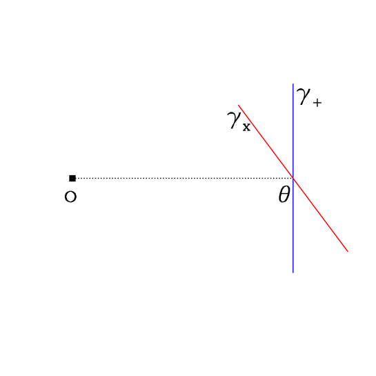
Figure 1.— The point $\o$ is used to define the $\gamma_{+}$ and $\gamma_{\times}$ components of the shear at point $\th$. The two rods indicate the ellipticity at $\th$ that would produce a positive $\gamma_{+}$ and $\gamma_{\times}$

Another important property of spin-2 fields is that they can be decomposed into two scalar potentials, one that is even under parity ($E$) and one that is odd ($B$) (Kamionkowski, Kosowsky & Stebbins (1997); Zaldarriaga & Seljak (1997); Crittenden et al. (2001); Schneider et al. (2002)). In fact for finite sky coverage or for maps with holes, there is a third family of modes, the ambiguous modes for which one does not have enough information to decide whether the contribution is coming from $E$ or from $B$ (Lewis, Challinor, & Turok (2002); Bunn, Zaldarriaga, Tegmark, & de Oliveira-Costa (2002)). Weak gravitational lensing only produces $E$ modes ($E$ is nothing but the projected mass density $\kappa$).

The properties under parity transformation of $\gamma_{+}$ and $\gamma_{\times}$ are different. As is clear from the definition, to obtain $\gamma_{\times}$ one has to rotate the coordinate system anticlockwise. This rotation changes direction when we do a parity transformation. This means that under parity $\gamma_{+}^{\prime}\rightarrow\gamma_{+}$ but $\gamma_{\times}^{\prime}\rightarrow-\gamma_{\times}$.

As a consequence of the difference in behavior of $\gamma_{+}$ and $\gamma_{\times}$ any estimator that contains an odd number of $\gamma_{\times}$ is odd under parity. The difference in their parity behavior will make some of the three-point functions vanish. To illustrate what this means we can consider the case of the three-point function for equilateral triangles. In principle there are 8 different combinations of the two shear components at the three points, however only four of them: $\mathop{\langle}\gamma_{+}\gamma_{+}\gamma_{+}\mathop{\rangle}$, $\mathop{\langle}\gamma_{+}\gamma_{\times}\gamma_{\times}\mathop{\rangle}$, $\mathop{\langle}\gamma_{\times}\gamma_{+}\gamma_{\times}\mathop{\rangle}$, $\mathop{\langle}\gamma_{\times}\gamma_{\times}\gamma_{+}\mathop{\rangle}$ contain any signal from weak lensing because they are the only four that are even under parity. We show patterns that produce positive values for these correlations in Fig. 2. For a discussion on how the difference in behavior under parity of the three-point functions of general configurations constraints their possible values see Takada & Jain 2002b .

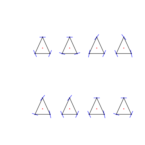
Figure 2.— The top row (from left to right) shows four shear patterns that would produce a positive value for $\mathop{\langle}\gamma_{+}\gamma_{+}\gamma_{+}\mathop{\rangle}$, $\mathop{\langle}\gamma_{\times}\gamma_{\times}\gamma_{+}\mathop{\rangle}$, $\mathop{\langle}\gamma_{\times}\gamma_{+}\gamma_{\times}\mathop{\rangle}$, $\mathop{\langle}\gamma_{+}\gamma_{\times}\gamma_{\times}\mathop{\rangle}$. The bottom row shows four shear patterns that would produce a positive value for $\mathop{\langle}\gamma_{\times}\gamma_{\times}\gamma_{\times}\mathop{\rangle}$, $\mathop{\langle}\gamma_{+}\gamma_{+}\gamma_{\times}\mathop{\rangle}$, $\mathop{\langle}\gamma_{+}\gamma_{\times}\gamma_{+}\mathop{\rangle}$, $\mathop{\langle}\gamma_{\times}\gamma_{+}\gamma_{+}\mathop{\rangle}$

.

Being able to separate combinations that have signal from those that do not is very important not to dilute the signal one is trying to measure when combining or binning the measured statistics to obtain a detection. Moreover for equilateral triangles for example the four odd combinations: $\mathop{\langle}\gamma_{\times}\gamma_{\times}\gamma_{\times}\mathop{\rangle}$, $\mathop{\langle}\gamma_{+}\gamma_{+}\gamma_{\times}\mathop{\rangle}$, $\mathop{\langle}\gamma_{\times}\gamma_{+}\gamma_{+}\mathop{\rangle}$, $\mathop{\langle}\gamma_{+}\gamma_{\times}\gamma_{+}\mathop{\rangle}$ may prove useful to monitor systematic problems in the data or to identify interesting physical effects such as clustering of the background sources, the effects of multiple scatterings, etc. (Bernardeau (1998); Jain, Seljak & White (2000)).

Any connected N-point function of the shear can be written as a linear combination of the connected N-point functions of the two potential $E$ and $B$. It is worth noting that in the case of connected N-point functions with odd number of legs there will be some configurations (such as those where the lenghts of all sides are equal) that can be separated into a set that only depends on the higher-order correlations of $E$ and a set that only depends on the higher moments of $B$ (assuming $E$ and $B$ are independent). We can argue this only on the basis of their bahavir under parity. The product of an odd number of $E$’s is even under parity while a product of an odd number of $B$’s is odd, thus the even parity N-point functions of the shear receive contributions only from $E$ and the odd ones only from $B$. For an N-point function with an even number of legs this is not true because the product of an even number of $E$s or $B$s is even under parity. The clearest example of this is the two-point correlation function where $\mathop{\langle}\gamma_{+}\gamma_{+}\mathop{\rangle}$ and $\mathop{\langle}\gamma_{\times}\gamma_{\times}\mathop{\rangle}$ receive contributions from both $\langle EE\rangle$ and $\langle BB\rangle$ while $\mathop{\langle}\gamma_{\times}\gamma_{+}\mathop{\rangle}$ is zero if there is no $E-B$ cross-correlation.

As we mentioned above the way to make a three-point function (or an N-point function for that matter) that is scalar is to contract the shear at the three points with some combination of the vectors that form the sides that transforms appropriately under rotations to cancel the spin of shear. That is we need to construct spin$-2$ combinations of these vectors. Our proposed scheme is easy to understand. For each member of $X$ we define $\tilde{\th}=\th-\o$ and we construct two spin$-2$ quantities,

$${\bf\bar{P}}_{+} = (\tilde{\theta}^{2}_{x}-\tilde{\theta}^{2}_{y},2\tilde{\theta}_{x}\tilde{\theta}_{y})/\tilde{\theta}^{2}$$

$$= (\cos 2\tilde{\phi},\sin 2\tilde{\phi})$$

$${\bf\bar{P}}_{\times} = (-2\tilde{\theta}_{x}\tilde{\theta}_{y},\tilde{\theta}^{2}_{x}-\tilde{\theta}^{2}_{y})/\tilde{\theta}^{2}$$ (3)

$$= (-\sin 2\tilde{\phi},\cos 2\tilde{\phi}).$$

The statistics we proposed are obtained by contracting the above quantities with the shear three-point function. For example,

$$\langle\gamma_{+}\gamma_{+}\gamma_{+}\rangle={\bar{P}}_{+}^{\mu_{1}}{\bar{P}}_{+}^{\mu_{2}}\bar{P}_{+}^{\mu_{3}}\langle\gamma_{\mu_{1}}\gamma_{\mu_{2}}\gamma_{\mu_{3}}\rangle,$$ (4)

where the index $\mu$ runs over the two components of the shear. The other three-point functions that we define are obtained by replacing some of the $\bar{P}_{+}$ by $\bar{P}_{\times}$. Finally we note that the vector $\tilde{\th}_{1}$ is nothing but $\tilde{\th}_{1}=[(\th_{1}-\th_{2})+(\th_{1}-\th_{3})]/3$, i.e. basically the sum of the vectors that define the sides of the triangle that cross at $\th_{1}$. The same is true for the other vertices.

3. Worked Examples

Our objective in this section is to get some intuition into how these higher-order correlations behave. To keep things simple we will just focus on the three-point function. To get some idea of how these functions behave we will work in the context of the halo model, i.e. the dark matter is assumed to be distributed in a collection of halos of different mass. Although analytic approximations and fits to numerical simulations exist for the profile of these halos and their mass function, this modeling is clearly simplistic to model the shear field as in reality halos are not spherical. This particularly is bound to affect the configuration dependence of the three-point function. Thus definite predictions will need more detailed modeling and comparison with direct measurements using numerical simulations.

Our aim in this paper is more modest, we only want to gain some insight into how these different three-point functions behave, if they are positive or negative for example. We will start by considering the simple case of lensing by a singular isothermal sphere. We do this because the calculation of the three-point function can be done analytically, and it provides a useful check on the numerical code used to do the same calculations in the halo model, presented in 3.2.

3.1. The Singular Isothermal Sphere

In this section we will calculate the three-point function that results from a single halo with a power-law density run. For definiteness we will write down formulas for a singular isothermal sphere (SIS), but other power laws can be calculated in analogous way. For a SIS the density $\rho(r)$ depends on distance from the center $r$ as $\rho(r)\propto r^{-2}$; therefore, both the projected mass density $\kappa$ and the shear $\gamma$ scale with projected separation as $r_{\perp}^{-1}$.

The shear pattern around a spherical halo is tangential centered at the origin of the halo which we will call ${\bf u}$. When defining the shear components at a point $\th$, we will need to rotate the shear elements so as to define them relative to the vector $\th-\o$. We will call this angle of rotation $\alpha$. We can write

$$\gamma_{+}(\th)={\cos(2\alpha)\over|\th-{\bf u}|}\ \ \ \ \ \gamma_{\times}(\th)={\sin(2\alpha)\over|\th-{\bf u}|}.$$ (5)

The cosine and sine of $2\alpha$ can be calculated in terms of

$$\cos(\alpha) = {(\th-{\bf u})\cdot(\th-\o)\over|\th-{\bf u}|\ |\th-\o|}$$ (6)

$$\sin(\alpha) = {\hat{z}\cdot[(\th-{\bf u})\times(\th-\o)]\over|\th-{\bf u}|\ |\th-\o|},$$ (7)

where $\hat{z}$ is the unit vector perpendicular to the plane of the sky. The three-point function $\zeta$ is obtained by integrating over the position of the center of the halo ${\bf u}$,

$$\zeta_{\gamma}^{+++}(l_{1},l_{2},l_{3}) = \int d^{2}{\bf u}{\cos(2\alpha_{1})\over|\th_{1}-{\bf u}|}{\cos(2\alpha_{2})\over|\th_{2}-{\bf u}|}{\cos(2\alpha_{3})\over|\th_{3}-{\bf u}|}$$ (8)

$$\zeta_{\gamma}^{+\times\times}(l_{1},l_{2},l_{3}) = \int d^{2}{\bf u}{\cos(2\alpha_{1})\over|\th_{1}-{\bf u}|}{\sin(2\alpha_{2})\over|\th_{2}-{\bf u}|}{\sin(2\alpha_{3})\over|\th_{3}-{\bf u}|},$$ (9)

where $l_{1},l_{2},l_{3}$ are the lengths of the triangle sides, $l_{1}^{2}=|\th_{2}-\th_{1}|^{2}$, $l_{2}^{2}=|\th_{3}-\th_{2}|^{2}$, $l_{3}^{2}=|\th_{1}-\th_{3}|^{2}$. There are two permutations of the second equation which give the remaining three-point correlators, $\zeta_{\gamma}^{\times+\times}$ and $\zeta_{\gamma}^{\times\times+}$.

To calculate Eqs. (8-9), we proceed as follows. First, for simplicity, we take the origin of coordinates to coincide with the center of mass, so $\o$ vanishes. We then write the ${\bf u}$ dependence inside the cosine and sine in Eqs. (6-7) in terms of ${\bf d}_{i}\equiv\th_{i}-{\bf u}$. This can be done simply using that

$${\bf u}\cdot\th_{i}=\frac{1}{2}\Big{(}u^{2}+|\th_{i}|^{2}-d_{i}^{2}\Big{)},$$ (10)

whereas the magnitude of ${\bf u}$ can be conveniently written as

$$u^{2}={1\over 3}(d_{1}^{2}+d_{2}^{2}+d_{3}^{2})-{1\over 9}(l_{1}^{2}+l_{2}^{2}+l_{3}^{2}).$$ (11)

Similarly we have $|\th_{1}|^{2}=(2l_{3}^{2}+2l_{1}^{2}-l_{2}^{2})/9$ and cyclic permutations. In this way, after appropriate translation in ${\bf u}$ the integrals in Eqs. (8-9) are of the form,

$$J(\nu_{1},\nu_{2},\nu_{3})=\int\frac{d^{2}{\bf u}}{(u^{2})^{\nu_{1}}[({\bf l_{1}}-{\bf u})^{2}]^{\nu_{2}}[({\bf l_{2}}-{\bf u})^{2}]^{\nu_{3}}}$$ (12)

which can be evaluated by using dimensional regularization techniques (see Scoccimarro 1997 and references therein) in terms of Apell’s hypergeometric function of two variables, ${\rm F}_{4}$, with the series expansion:

$${\rm F}_{4}(a,b;c,d;x,y)=\sum_{i=0}^{\infty}\sum_{j=0}^{\infty}\frac{x^{i}y^{j}}{i!\ j!}\ \frac{(a)_{i+j}(b)_{i+j}}{(c)_{i}(d)_{j}},$$ (13)

where $(a)_{i}\equiv\Gamma(a+i)/\Gamma(a)$. In our case, the arguments of $F_{4}$ have a special symmetry that allows us to write them in terms of regular hypergeometric functions,

$$F_{4}[\alpha,\gamma+\gamma^{\prime}-\alpha-1,\gamma,\gamma^{\prime};x(x-1),y(y-1)]=$$

$$F(\alpha,\gamma+\gamma^{\prime}-\alpha-1,\gamma,x)\times F(\alpha,\gamma+\gamma^{\prime}-\alpha-1,\gamma^{\prime},y),$$

which can be easily evaluated on the computer using MATHEMATICA. Figure 3 shows the results for different triangle configurations. Since the SIS is scale-free, the overall size of the triangle scales the results by a factor, so we take $l_{1}\equiv 1$. The top panel shows the four $\zeta_{\gamma}$’s for $l_{2}=l_{1}$ as a function of the angle $\phi$ between ${\bf l}_{1}$ and ${\bf l}_{2}$. We see that for most of the triangles ($\phi\gtrsim 0.3\pi$), the signal is dominated by $\zeta_{\gamma}^{+++}$, with a maximum close to equilateral triangles ($\phi=2\pi/3$). On the other hand, the three contributions involving $\gamma_{\times}$ are generally smaller in magnitude.

This can be understood geometrically from Fig. 4. Let us consider the halo center to be inside the triangle, which minimizes the distances to the vertices and thus maximizes the signal. Since $\cos(2\alpha)>0$ for $|\alpha|<\pi/4$, as long as the internal angles of the triangle are smaller than $\pi/2$, $\zeta_{\gamma}^{+++}$ is positive. As $\phi\rightarrow\pi$, $\alpha_{2}\rightarrow 0$, whereas $|\alpha_{1}|=|\alpha_{3}|$ cannot be larger than $\pi/2$; thus $\zeta_{\gamma}^{+++}$ remains positive as $\phi\rightarrow\pi$. On the other hand, as $\phi\rightarrow 0$, $\alpha_{1}=\alpha_{3}\rightarrow 0$, whereas $|\alpha_{2}|\rightarrow\pi$ if ${\bf u}$ is off center; that explains why $\zeta_{\gamma}^{+++}$ becomes negative as $\phi\rightarrow 0$.

For the three other three-point functions involving $\gamma_{\times}$, things are more subtle. Since $\sin(2\alpha)$ changes sign at $\alpha=0$, $\gamma_{\times}$ can be positive or negative depending on the location of ${\bf u}$ relative to the bisector of the vertex. As a result moving ${\bf u}$ inside the triangle leads to cancellations, and thus smaller amplitude for $\zeta_{\gamma}$’s. The bottom panel in Fig. 3 shows results for configurations in which $l_{2}=2l_{1}$. A similar pattern is seen, where for isosceles triangles $\phi\approx 0.6\pi$ the $\zeta_{\gamma}^{+++}$ is positive and maximum, whereas the remaining three contributions are smaller, becoming comparable only for collapsed triangles which can avoid cancellations.

The physical interpretation of the different amplitudes is sketched in Fig. 5. In the top (bottom) row we show patterns that would produce positive (negative) values for $\zeta_{\gamma}^{+++}$, $\zeta_{\gamma}^{\times\times+}$, $\zeta_{\gamma}^{\times+\times}$, and $\zeta_{\gamma}^{+\times\times}$ from left to right, respectively. It is clear from the figure that the top examples correspond to patters that would be produced by overdensities and the bottom patterns would be produced by underdensities. We indicate with a square the region where the overdensity (underdensity) should be located to produce such pattern.

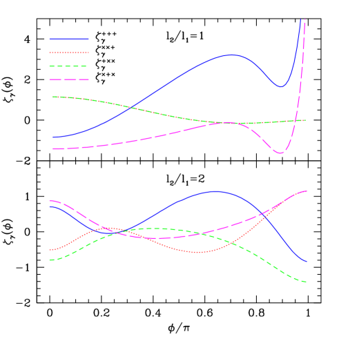
Figure 3.— The shear three-point functions $\zeta_{\gamma}(l_{1},l_{2},l_{3})$ for the case of isothermal sphere halos, as a function of the angle $\phi$ between ${\bf l}_{1}$ and ${\bf l}_{2}$ for $l_{2}=l_{1}$ (top panel) and $l_{2}=2l_{1}$ (bottom panel). Different line styles correspond to the four shear correlators, as labeled in the top panel.

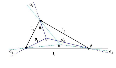
Figure 4.— Definition of triangle variables. We characterize the shear generated by a halo with center at ${\bf u}$ by measuring its components with respect to the center of mass of the triangle, denoted by $\o$.

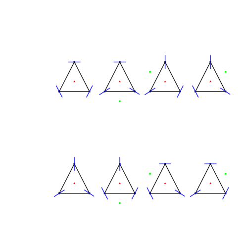
Figure 5.— Examples of shear patterns generated at the vertices of equilateral triangles by overdensities (top panel) and underdensities (bottom panel) located at the position denoted by square symbols. From left to right, contributions to $\zeta_{\gamma}^{+++}$, $\zeta_{\gamma}^{\times\times+}$, $\zeta_{\gamma}^{\times+\times}$, and $\zeta_{\gamma}^{+\times\times}$ (vertices labeled anticlockwise starting from bottom-left vertex). Note that on the left-most plots, the density perturbation is located at the center of the triangle.

3.2. Superposition of NFW profiles

In this section we will calculate the three-point functions using the halo model (Peacock & Smith 2000, Seljak 2000, Ma & Fry 2000, Scoccimarro et al. 2001). For simplicity we will restrict ourselves to the one-halo term which dominates on the small scales where the three-point function of the shear is easiest to measure in observations. For examples of calculations of weak gravitational lensing higher-order moments in the context of the halo model see Cooray & Hu (2001) and Takada & Jain 2002a . Measurements of higher-order moments of the convergence field in numerical simulations are given in Jain, Seljak & White (2000), White & Hu (2000); Van Waerbeke et al (2001) also present results for aperture mass statistics which is directly related to the cosmic shear.

Under our assumptions the averaged shear can be written as an integral over radial distance ($d\chi=c\ dt/a$), mass ($M$) and angular location (${\bf u}$) of halos,

$$\zeta_{\gamma}(l_{1},l_{2},l_{3}) = \int d\chi\ d_{A}^{2}(\chi)\int dM{dn\over dM}\int d^{2}{\bf u}$$

$$\tilde{\gamma}({\bf u},\th_{1},M,\chi) \tilde{\gamma}({\bf u},\th_{2},M,\chi)\ \ \tilde{\gamma}({\bf u},\th_{3},M,\chi),$$ (15)

where $a$ is the expansion factor of the universe, $d_{A}$ is the comoving angular diameter distance, ${dn/dM}$ is the mass function of halos. We have introduced the notation $\tilde{\gamma}({\bf u},\th,M,\chi)$ to indicate the shear produced at position $\th$ by a halo at radial distance $\chi$ and angular position ${\bf u}$. Note that for convenience we are using the same symbol regardless of whether $\gamma_{+}$ or $\gamma_{\times}$ is involved.

To obtain an estimate for the three-point function we will evaluate Eq. (3.2) assuming that the background sources used to measure the shear are all at redshift $z_{s}=1$ and that the cosmological model is the so called LCDM model ( $\Omega_{m}=0.3$, $\Omega_{\Lambda}=0.7$, $h=0.7$, $\sigma_{8}=0.9$ and $n=1$). We will assume that the mass function of halos is that given by Sheth & Tormen (1999); Jenkins et al. (2001) and that dark matter halos have an NFW profile nfw (Navarro, Frenk & White 1997). In particular, we use

$$\rho(r)={\rho_{s}\over r/r_{s}(1+r/r_{s})^{2}}$$ (16)

where $r$ is measured in comoving coordinates and $r_{s}$ is related to the virial radius of the halo by the concentration parameter $c$, $r_{s}=r_{vir}/c$. The mass of the halo is given by $M=4\pi\rho_{s}r_{vir}^{3}(\ln(1+c)-c/(1+c))/c^{3}$. The virial radius is calculated using that $M=4\pi/3r_{vir}^{3}\bar{\rho}_{0}\Delta(z)$ with $\bar{\rho}_{0}$ the mean density of the universe today and $\Delta(z)$ the overdensity of collapse as a function of redshift (ie. $\Delta(z=0)\approx 340$ for LCDM). For the concentration we take $c(M,z)=9/(1+z)(M/M_{*})^{-0.13}$ bullock (Bullock et al. 2001), where $M_{*}$ is the mass contained in a sphere of radius $R_{*}$ at which the variance of the density is one ($R_{*}\approx 3.14\ h^{-1}{\rm Mpc}$ for LCDM).

The shear produced by an NFW profile at the origin is calculated as follows. The shear is expressed in terms of second derivatives of the gravitational potential $\psi$, $\gamma_{1}=1/2(\psi_{xx}-\psi_{yy})$ and $\gamma_{2}=\psi_{xy}$. The gravitational potential satisfies

$$\nabla^{2}_{{\bf u}}\psi = 2\kappa(u)$$

$$\kappa(u) = {1\over a\Sigma_{\rm crit}}\int dz\ \rho(\sqrt{u^{2}d^{2}_{A}(\chi)+z^{2}})$$ (17)

where $1/\Sigma{\rm crit}=4\pi Gd_{A}(\chi)d_{A}(\chi-\chi_{s})/c^{2}d_{A}(\chi_{s})$, $\chi$ gives the radial position of the halo and $\chi_{s}$ that of the background sources. Equation (3.2) is easily integrated to obtain $\psi$ because $\kappa$ is only a function of $u$. Once the shear is obtained for a halo at the origin, we obtain $\tilde{\gamma}({\bf u},\th,M,\chi)$ with a coordinate transformation. A similar evaluation for the SIS to compare with the results obtained by the method of the previous section gives a useful check to our numerical integration code.

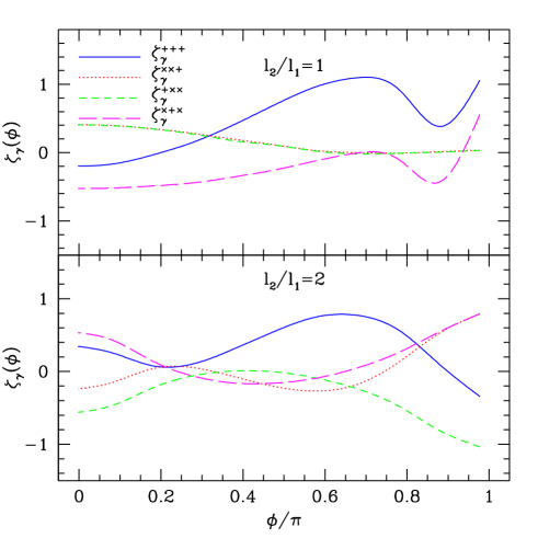
Figure 6.— Even components of the three-point function of the shear calculated using the 1-halo term for LCDM. The top (bottom) panel shown the case $l_{1}=l_{2}=2^{\prime}$ ($l_{1}=2^{\prime}$, $l_{2}=4^{\prime}$).

Figure 6 shows the results of our calculation for some specific triangles. In the top panel $l_{1}=l_{2}=2^{\prime}$ and in the bottom panel the case $l_{1}=2^{\prime}$ and $l_{2}=4^{\prime}$. The similarities with the results for the SIS are striking, thus we can understand the dependence of each of the curves with $\phi$ in exactly the same way.

The expected level of $\zeta_{\gamma}$ on arcminute scales is $\zeta_{\gamma}\sim 10^{-6}$. We estimate the number of triangles ($N_{T}$) needed to detect the three-point function in a particular configuration above the noise produced by the intrinsic ellipticity of the background galaxies as follows. If the typical ellipticity of the background galaxies is $\sim 0.3$ then the typical noise added to each components of the intrinsic shear is $\sigma\sim 0.3/\sqrt{2}\sim 0.2$. The expected noise in the three-point function is then $\sigma^{3}/\sqrt{N}_{T}$. This implies that one needs roughly $N_{T}\sim 6.5\times 10^{7}$ triangles of a particular shape to estimate the three-point function. In a survey covering a solid angle $\Omega$ with a mean desity of galaxies $\bar{n}$ there are roughly $N_{T}=\bar{n}\Omega\ (\pi R^{2}\bar{n})^{2}/6$ triangles with sides of scale $R$. Current surveys have about 20 galaxies/${\rm arcmin}^{2}$ implying that in a few square degrees there are enough triangles with sides of order an arcminute to detect this signal.

4. Summary and Discussion

In this paper we have introduced a new way of defining higher-order correlation functions of a spin-2 field such as the weak lensing shear or the CMB polarization by using the “center of mass” of the configuration as the origin from which the components of the shear are defined. In principle for an $N$-point function there are $2^{N}$ different statistics of the shear. We have shown that these statistics can be divided according to their behavior under parity transformation and that one does not expect a cosmological signal in the odd ones for some configurations, such as for equilateral triangles.

In order to gain intuition about the behavior of these statistics we calculated the four even three-point functions under some simple assumptions. We calculated analytically what would be expected to be produced by an ensemble of singular isothermal spheres. We showed that $\zeta_{\gamma}^{+++}$ is positive and expected to carry the bulk of the signal for triangles that are not too elongated. For elongated triangles we showed that all four three-point functions have similar values but some of them are positive and others are negative. If two of the points are very close to each another $\zeta_{\gamma}^{+++}$ and $\zeta_{\gamma}^{\times+\times}$ carry most of the signal.

We estimated the three-point functions in the context of the halo model using the contributions from the one-halo term, which should be a reasonable approximation at small angular scales. We showed that the configuration dependence in this case is almost identical to that found for the SIS. We estimated that in order to detect a signal above the noise (due to the intrinsic ellipticity of galaxies) at scales of order of one arcminute a survey of a few square degrees is necessary.

Clearly both the fact that we restricted ourselves to the one-halo term and that we assumed the halos to be spherical will affect the behavior of the three-point function. A detailed study using numerical simulations will be needed to improve upon the calculation presented here (Benabed, Scoccimarro & Zaldarriaga, in preparation). The potential rewards of detecting a non-Gaussian signal in the shear maps are enourmous and the tantalizing detections reported so far (Bernardeau, Mellier & Van Waerbeke 2002b ) make this a very exciting time to study these issues in detail.

When this paper was under completion, a similar proposal for calculating the shear three-point function was put forward by Schneider & Lombardi (2002).

Acknowledgments: We thank Mashiro Takada and Bhuvnesh Jain for pointing out an error in the first version of the manuscript. MZ is supported by David and Lucille Packard Foundation Fellowship for Science and Engeneering and NSF grant AST-0098506. RS is supported by NASA ATP grant NAG5-12100. MZ and RS are supported by NSF grant PHY-0116590.

References

- Bacon et al. (2000) Bacon, D.J., Refregier, A.R. & Ellis, R.S. 2000, MNRAS, 318, 625
- Bernardeau, Van Waerbeke & Mellier (1997) Bernardeau, F., Van Waerbeke, L. & Mellier, Y. 1997, å, 345, 17
- Bernardeau (1998) Bernardeau, F. 1998, A&A, 338, 375
- (4) Bernardeau, F., Van Waerbeke, L. & Mellier, Y. 2002a, astro-ph/0201029
- (5) Bernardeau, F., Mellier, Y. & Van Waerbeke, L. 2002b, astro-ph/0201032
- (6) J.S. Bullock, T.S. Kolatt, Y. Sigad, R.S. Somerville, A.V. Kravtsov, A.A. Klypin, J.R. Primack, A. Dekel, 2001, MNRAS, 321, 559
- Bunn, Zaldarriaga, Tegmark, & de Oliveira-Costa (2002) Bunn, E. F., Zaldarriaga, M., Tegmark, M., & de Oliveira-Costa, A. 2002, astro-ph/0207338
- Cooray, Hu & Miralda-Escudé (2000) Cooray, A. Hu, W. Miralda-Escudé, J. 2000, ApJ, 535, L9
- Cooray & Hu (2001) Cooray, A. & Hu, W. 2001, ApJ, 548, 7
- Cooray & Sheth (2002) Cooray, A. & Sheth, R.K. 2002, astro-ph/0206508
- Couchman et al (1999) Couchman, H.M.P. Barber, A.J. & Thomas, P.A. 1999, MNRAS, 308, 180
- Crittenden et al. (2001) Crittenden, R. G., Natarajan, P., Pen, U. L., & Theuns, T. 2001, ApJ, 559, 552
- Hui (1999) Hui, L. 1999, ApJ, 519, L9
- Jain & Seljak (1997) Jain, B. & Seljak, U. 1997, ApJ, 484, 560
- Jain, Seljak & White (2000) Jain, B., Seljak, U. & White, S.D.M. 2000, ApJ, 530, 547
- Jenkins et al. (2001) A. Jenkins, C.S. Frenk, S.D.M. White, J.M. Colberg, S. Cole, A.E. Evrard, H.M.P. Couchman, N. Yoshida, 2000, MNRAS, 321, 372
- Kaiser (1992) Kaiser N. 1992, ApJ388, 272
- Kaiser et al. (1994) Kaiser N., Squires G., Fahlman G. & Woods D., 1994, in clusters of Galaxies, Eds. F. Durret, A. Mazure, J. Tran Thanh Van, Editions Frontieres, vol. 437, 56
- Kaiser et al (2000) Kaiser, N., Wilson, G. & Luppino, G. 2000, astro-ph/0003338
- Kamionkowski, Kosowsky & Stebbins (1997) Kamionkowski M., Kosowsky A. & Stebbins A. 1997, Phys. Rev. D, 55, 7368
- Lewis, Challinor, & Turok (2002) Lewis, A., Challinor, A., & Turok, N. 2002, Phys. Rev. D, 65, 23505
- Ma & Fry (2000) Ma, C.-P. &Fry, J.N. 2000, ApJ, 543, 503
- Miralda-Escudé (1991) Miralda-Escude, J. 1991, ApJ, 380, 1
- (24) Navarro, J.F., Frenk, C.S. & White, S.D.M. 1997, ApJ, 490, 493
- Peacock & Smith (2000) Peacock, J.A. & Smith, R.E. 2000, MNRAS, 318, 1144
- Schneider, van Waerbeke, Jain, & Kruse (1998) Schneider, P., van Waerbeke, L., Jain, B., & Kruse, G. 1998, MNRAS, 296, 873
- Schneider et al. (2002) Schneider, P., van Waerbeke, L., Kilbinger, M., & Mellier, Y. 2002, astro-ph/0206182
- Schneider & Lombardi (2002) Schneider, P. & Lombardi, M. 2002, astro-ph/0207454
- Scoccimarro (1997) Scoccimarro, R. 1997, ApJ, 487, 1
- Scoccimarro & Frieman (1999) Scoccimarro, R. & Frieman, J. 1999, ApJ, 520, 35
- Scoccimarro et al. (2001) Scoccimarro, R., Sheth, R.K., Hui, L., Jain, B. 2001, ApJ, 546, 20
- Seljak (2000) Seljak, U. 2000, MNRAS, 318, 203
- Sheth & Tormen (1999) Sheth, R.K. & Tormen, B. 1999, MNRAS, 308, 119
- (34) Takada, M. & Jain, B. 2002, astro-ph/0209167
- (35) Takada, M. & Jain, B. 2002, astro-ph/0210261
- Van Waerbeke, Bernardeau & Mellier (1999) Van Waerbeke, L. Bernardeau, F. Mellier, Y. 1999, å, 34, 15
- Van Waerbeke et al. (2000) L. Van Waerbeke, Y. Mellier, T. Erben, J.C. Cuillandre, F. Bernardeau, R. Maoli, E. Bertin, H.J. Mc Cracken, O. Le F vre, B. Fort, M. Dantel-Fort, B. Jain, P. Schneider, 2000, å, 358, 30
- Van Waerbeke et al. (2001) Van Waerbeke, L., Hamana, T., Scoccimarro, R., Colombi, S., Bernardeau, F. 2001, MNRAS, 322, 918
- White & Hu (2000) White, M. & Hu, W. 2000, ApJ, 537, 1
- Wittman et al (2000) D.M. Wittman, J.A. Tyson, D. Kirkman, I. Dell’Antonio, G. Bernstein, 2000, Nature, 405, 143
- Zaldarriaga & Seljak (1997) Zaldarriaga M. & Seljak U. 1997, Phys. Rev. D, 55, 1830