1 ABSTRACT

In the framework of the study of extragalactic radio sources, we will focus on the importance of the spatial resolution at different wavelengths, and of the combination of observations at different frequency bands. In particular, a substantial step forward in this field is now provided by the new generation X-ray telescopes which are able to image radio sources in between 0.1–10 keV with a spatial resolution comparable with that of the radio telescopes (VLA) and of the optical telescopes. After a brief description of some basic aspects of acceleration mechanisms and of the radiative processes at work in the extragalactic radio sources, we will focus on a number of recent radio, optical and X–ray observations with arcsec resolution, and discuss the deriving constraints on the physics of these sources.

2 INTRODUCTION

This contribution is focussed on some basic concepts regarding the study of the non–thermal emission from extragalactic radio sources based on a broad band, multifrequency approach. The principal difficulty in this study arises by the different sensitivity and spatial resolution of the instruments in different bands. Radio telescopes easily reach sub–arcsec spatial resolutions and can image very faint sources by relatively short observations. On the other hand, optical telescopes generally have only arcsec spatial resolution so that combined radio – optical studies are limited by the lower spatial resolution of the optical telescopes. Although, the problem is alleviated by making use of optical HST observations, it still remains to a certain degree. In order to extend this approach to higher energies, X–ray telescopes with arcsec resolution (at least) and good sensitivity are required. Neverthless the poor spatial resolution of the past X–ray observatories, pioneeristic studies in this direction have been attempted in the last 10-20 years with combined radio (and optical) and Einstein or ROSAT X–ray observations.

TABLE 1.  : X-ray Observatories

  Satellite Instrument Flux$\rightarrow$1 cts/s Energy Band Resolution (erg/s/cm²) (keV) (arcsec)  Einstein HRI 1.6E-10 0.5-4.0 4 IPC 2.8E-11 0.5-4.0  ROSAT HRI 3.7E-11 0.5-2.4 3* PSPC 1.4E-11 0.5-2.4 20  ASCA SIS 3.3E-11 0.4-12 180 GIS 3.8E-11 0.4-12 180  BeppoSAX MECS 8.1E-11 1.3-10 60 PDS 9.5E-11 13-80
 Chandra HRC-I 2.8E-11 0.4-10 0.5
ACIS-I 1.1E-11 0.4-10 0.5
  

Notes: Column 3, Flux$\rightarrow$ is the flux (erg/s/cm²) necessary to have 1 cts/s in the detector. Column 5: (*) means that the spatial resolution results affected by errors in the aspect solution associated with the wobble of the space craft.

More recently, a substantial step forward has been achieved thanks to the advent of the new generation X–ray satellites: Chandra and XMM-Newton. In Tab.1 we report the main capabilities of a selection of past X–ray observatories compared with those of Chandra: the abrupt increase of the spatial resolution combined with the high effective area of Chandra represent a ‘new revolution’ in astrophysics (data taken from Cox, 1999). For the first time it is now possible to investigate the X–ray properties of extragalactic radio sources performing spatially resolved spectroscopy over a relatively large energy band (about 0.4–10 keV). Chandra allows us to obtain images with $\leq$arcsec spatial resolution, comparable with the typical resolution of the VLA radio images and of the optical telescopes and thus it is a tool to perform, for the first time, multiwavelength studies from the radio band to the X–rays.

As we will show in this contribution, the high resolution broad band study of non–thermal emission from the extragalactic radio sources allows us to sample the emission due to very different portions of the spectrum of the relativistic electrons or to study the emission due to different emitting mechanisms at work in the observed regions. After the first 3 years of new Chandra observations, it is now clear that the scenarios describing these objects should now be partially revisited.

In Sect.3 we discuss some theoretical aspects related to the relativistic plasma in extragalactic radio sources. More specifically, in Sects. 3.1–3.3 we report the basic concepts of particle acceleration and discuss the resulting spectrum of the relativistic electrons in the framework of the standard shock acceleration scenario. In Sect. 3.4 we introduce the non–thermal emitting mechanisms. In particular, we focus on the sampling of the spectrum of the emitting electrons provided by the observations at different frequencies. In Sect. 3.5 we review the basic methods to derive the energetics of the relativistic plasma in the extragalactic radio sources. Finally, in Sect.4 we concentrate on the most recent high resolution multiwavelength studies of extragalactic radio sources. Our ‘biased’ review is mainly focussed on the new Chandra observations of radio lobes, radio jets and radio hot spots. Combining the data with the methods showed in Sect. 3, we discuss on the new constraints on the shape of the low and high energy end of the electron spectrum, on the kinematics of radio jets, and on the energetics of extragalactic radio sources.

3 PARTICLE ACCELERATION AND RADIATIVE MECHANISMS

In this Section we give the basic concepts of the particle acceleration and of the time evolution of the energy of the particles. We focus our attention on the case of electrons which are responsible for the observed non–thermal emission. The acceleration of electrons to high energies in various environments is a problem of widespread interest in astrophysics. Indeed, the synchrotron emission of jets in a large number of extragalactic radio sources (e.g., Miley, 1980; Fomalont, 1983; Venturi, this proceedings) requires in situ acceleration of electrons because of the short synchrotron life–times (e.g., Rees, 1978; Bicknell & Melrose, 1982). Also the radio luminosity of supernova remnants and their broad band spectrum (e.g., Clark & Caswell, 1976; Dickel, 1983) suggest that electrons are accelerated to high energy in these cases. Finally, the diffuse Mpc–size radio emission discovered in an increasing number of clusters of galaxies (e.g., Feretti & Giovannini 1996) requires large scale in situ acceleration of protons and electrons (e.g., Jaffe 1977; Tribble 1993; Sarazin 1999; Blasi 2001; Brunetti et al. 2001a; Petrosian 2001).

The basic goal of this Section is simply to show, based on general theoretical arguments, that the energy distribution of the relativistic electrons in extragalactic radio sources cannot be a simple power law. Although a power law energy distribution is commonly assumed in the literature, here we will point out that this approximation cannot be adopted in a broad band, multiwavelength (radio to X–ray observations) approach, and further that the observations can be used to constrain the energy distribution of the emitting electrons. In this way we will test the acceleration theories.

3.1 Competing mechanisms at work

The relativistic electrons in extragalactic radio sources are subject to several inescapable processes that change their energy with time. For a general description of the leading mechanisms at work we refer the reader to classical books (e.g., Ginzburg 1969; Pacholczyk 1970; Rybicki & Lightman 1979; Melrose 1980).

Here, it is important to underline that the efficiency of these processes is related to the energy of the electrons in a way that depends on the particular process. As a consequence, the time evolution of relativistic electrons at different energies is expected to be dominated by different processes. In the following, we give some basic relationships:

$\bullet$ Relativistic electrons with Lorentz factor $\gamma$ mixed with a thermal plasma lose energy via ionization losses and Coulomb collisions; for relativistic electrons one has :

$$\left({{d\gamma}\over{dt}}\right)_{\rm ion}^{-}=-1.2\times 10^{-12}n\left[1+{{{\rm ln}(\gamma/n)}\over{75}}\right]$$ (1)

where $n$ is the number density of the thermal plasma.

$\bullet$ If the relativistic electrons are confined into an expanding region, they lose energy via adiabatic expansion:

$$\left({{d\gamma}\over{dt}}\right)_{\rm ex}^{-}=-{1\over{R}}{{dR}\over{dt}}\gamma\sim 10^{-11}\gamma{{v_{\rm ex}(t)}\over{c}}{1\over{R(t)_{\rm kpc}}}$$ (2)

where $v_{\rm ex}$ and $R$ are the expansion velocity and dimension of the region, respectively.

$\bullet$ Relativistic electrons in a magnetic field $B$ lose energy via synchrotron radiation :

$$\left({{d\gamma}\over{dt}}\right)_{\rm syn}^{-}=-1.9\times 10^{-9}\gamma^{2}B^{2}\sin^{2}\theta$$ (3)

and via inverse Compton scattering with photons (of energy density $\omega_{\rm ph}$); in the Thompson regime, one has:

$$\left({{d\gamma}\over{dt}}\right)_{\rm ic}^{-}=-3.2\times 10^{-8}\gamma^{2}\omega_{\rm ph}$$ (4)

$\bullet$ Finally, the electrons can be accelerated/re–accelerated by several mechanisms. The most commonly considered in the literature are the Fermi and Fermi–like processes. It should be stressed that, in general, such mechanisms are stochastic processes, i.e., given an initial monoenergetic electron distribution, they not only produce a net increase of the energy of the electrons but also a broadening of the energy distribution. Thus the effect of a reacceleration mechanism on an initial energy distribution can be described by the combination of a systematic acceleration of the electrons and of a ’statistical’ broadening of the resulting energy distribution.

Two relevant cases are:

a) acceleration due to MHD turbulence; this is discussed in detail in a number of papers and classical books (e.g., Melrose 1980). If the resonance scattering condition (e.g., Eilek & Hughes 1991) is satisfied (this in general requires already relativistic electrons, e.g. Hamilton & Petrosian 1992), turbulent Alfven waves can accelerate electrons via resonant pitch angle scattering. For a power law energy spectrum of the Alfven waves:

$$P(k)=b{{B^{2}}\over{8\pi}}{{s-1}\over{k_{o}}}\left({{k\over{k_{o}}}}\right)^{-s}$$ (5)

in the range $k_{o}<k<k_{\rm max}$, where $k$ is the wave number ($k_{o}<<k_{\rm max}$) and $b$ is a normalization factor indicating the fractional energy density in waves, the systematic energy gain is (e.g., Isenberg 1987; Blasi 2000; Ohno et al. 2002):

$$\left({{d\gamma}\over{dt}}\right)_{\rm A-tur}^{+}\sim(s+2){\xi_{\rm A}}\gamma^{s-1}$$ (6)

where

$${\xi_{\rm A}}={{s-1}\over{s(s+2)}}{{\pi bk_{o}{v_{\rm A}}^{2}}\over{c}}\left({{eB}\over{m_{\rm e}c^{2}k_{o}}}\right)^{2-s}$$ (7)

and where $v_{\rm A}$ is the Alfven velocity.

MHD turbulence can also accelerate relativistic particles in radio sources via Fermi–like processes (e.g., Lacombe 1977; Ferrari et al. 1979). Under the simple assumption of a quasi–monochromatic turbulent scale (e.g., Gitti et al. 2002) the systematic energy gain is :

$$\left({{d\gamma}\over{dt}}\right)_{\rm F-tur}^{+}\simeq 4\times 10^{-11}\gamma{{{v_{\rm A}}^{2}}\over{l}}\left({{\delta B}\over{B}}\right)^{2}$$ (8)

where $l$ is the distance between two peaks of turbulence and $\delta B/B$ is the fluctuation in a peak of the field intensity with respect to the average field strength.

b) acceleration in a shock; (e.g., Meisenheimer et al. 1989); one has :

$$\left({{d\gamma}\over{dt}}\right)_{\rm sh}^{+}\simeq\gamma{{{U_{-}}^{2}c}\over{r}}\left({{r-1}\over{r\lambda_{+}+\lambda_{-}}}\right)$$ (9)

where $U_{-}$ is the velocity of the plasma in the region before the shock discontinuity (measured in the shock frame and in unit of $c$), $r$ is the shock compression ratio, and $\lambda_{\pm}$ is the mean diffusion length of the electrons in the region before ($-$) and after ($+$) the shock. Assuming a similar $B$–field configuration and strength before and after the shock (i.e. at some distance from the shock in the pre– and post–shock region) Eq.(9) can be generalized as :

$$\left({{d\gamma}\over{dt}}\right)_{\rm sh}^{+}\simeq\gamma{{{U_{-}}^{2}}\over{r}}\left({{r-1}\over{r+1}}\right){1\over{3{\cal K}(\gamma)}}$$ (10)

where ${\cal K}(\gamma)$ is the spatial diffusion coefficient which depends on the physical conditions.

In the relevant astrophysical cases the time evolution of the energy of the electrons is given by the combination of several mechanisms, i.e. :

$$\left({{d\gamma}\over{dt}}\right)=\sum_{i}^{..}\left({{d\gamma}\over{dt}}\right)_{i}^{-}+\sum_{i}^{..}\left({{d\gamma}\over{dt}}\right)_{i}^{+}$$ (11)

Figure 1.  : A sketch of the efficiency of acceleration (solid line) and loss (dashed lines) processes is shown, as a function of the Lorentz factor of the electrons. The artificial knee introduced in the IC losses at $\gamma>10^{7}$ simulates the effect of the KN cross section.

In Fig.1 we report $d\gamma/dt$ due to the above processes as a function of $\gamma$ for representative physical conditions. It is clear that the different processes dominate in different energy regions with the Coulomb losses being especially important at low energies. In addition, due to its dependence on the energy ($\propto\gamma$), the Fermi–like acceleration can be an efficient process in a restricted energy band, whereas Coulomb and radiative losses in general, prevent electron acceleration at lower and higher energies, respectively.

3.2 The basic equations of particle evolution

In order to consider the general evolution of the particle spectrum, a kinetic theory approach is suitable (e.g., Melrose 1980; Livshitz & Pitaevskii 1981; Blandford 1986; Blandford & Eichler 1987; Eilek & Hughes 1991, and reference therein). Given $f({\bf p},..)$, the distribution function of the electrons (i.e. $f({\bf p},..)d{\bf p}$ is the number of electrons in the element $d{\bf p}$ of the momentum space), the description of the behaviour of this distribution function is given by a Boltzman equation:

$${{df({\bf p})}\over{dt}}=\left({{\partial f}\over{\partial t}}\right)_{\rm coll}+\left({{\partial f}\over{\partial t}}\right)_{\rm diff}$$ (12)

where, the total time derivative is to be interpreted according to:

$${{d}\over{dt}}\rightarrow{{\partial}\over{\partial t}}+{\bf v}\cdot{{\partial}\over{\partial{\bf r}}}+{\bf F}\cdot{{\partial}\over{\partial{\bf p}}}$$ (13)

where ${\bf v}$ is the particle velocity, and ${\bf F}=d{\bf p}/dt$ the force acting on the particles.

The diffusion term in Eq.(12) describes spatial diffusion, while the collision term accounts for all the physics of collisions and scattering (e.g., radiative losses, interaction with waves and shocks, Coulomb collisions). A general, stochastic acceleration may be thought of as a diffusion in the momentum space given by a diffusion coefficient, $D_{pp}$, so that in case of no spatial diffusion and no losses, Eq.(12) can be written as:

$${{df({\bf p})}\over{dt}}={{\partial}\over{\partial p_{i}}}[(D_{pp})_{ij}({\bf p}){{\partial}\over{\partial p_{i}}}f({\bf p})]$$ (14)

If isotropy of the scattering waves and electrons is assumed, $f({\bf p})d{\bf p}=4\pi p^{2}f(p)dp$ and Eq.(12) can be written as (e.g., Melrose 1980; Eilek & Hughes 1991):

$${{\partial}\over{\partial t}}f({\bf r},p,t)+{{\partial}\over{\partial x_{i}}}[{\cal K}_{ij}{{\partial}\over{\partial x_{j}}}f({\bf r},p,t)]={1\over{p^{2}}}{{\partial}\over{\partial p}}[{\cal S}p^{4}f({\bf r},p,t)$$

$$+p^{2}D_{pp}{{\partial}\over{\partial p}}f({\bf r},p,t)+p^{2}I(p)f({\bf r},p,t)]+Q({\bf r},p,t)$$ (15)

where we have considered the effect of the synchrotron and inverse Compton losses ($dp/dt=-{\cal S}p^{2}$), of the Coulomb losses ($dp/dt=-I(p)$) and considered a general form for the spatial diffusion of the electrons (${\cal K}$ being the spatial diffusion coefficient). A term accounting for electron injection (injection rate = $Q$) has also been introduced.

Eq.(15) can be also written in the energy space. For an isotropic distribution of the momenta of the relativistic electrons, the electron spectrum is $N(\epsilon)=4\pi p^{2}f(p)dp/d\epsilon$ and one has :

$${{\partial}\over{\partial t}}f({\bf r},p,t)={{\rm c}\over{4\pi p^{2}}}{{\partial}\over{\partial t}}N({\bf r},\epsilon,t)$$ (16)

$${{\partial}\over{\partial p}}[{\cal S}p^{4}f({\bf r},p,t)]={{\rm c}\over{4\pi}}{{\partial}\over{\partial p}}[{\cal S}p^{2}N({\bf r},\epsilon,t)]$$ (17)

$${{\partial}\over{\partial p}}[p^{2}I(p)f({\bf r},p,t)]={{\rm c}\over{4\pi}}{{\partial}\over{\partial p}}[I(p)N({\bf r},\epsilon,t)]$$ (18)

$${{\partial}\over{\partial p}}[p^{2}D_{pp}{{\partial}\over{\partial p}}f({\bf r},p,t)]={{\rm c}\over{4\pi}}{{\partial}\over{\partial p}}[D_{pp}{{\partial}\over{\partial p}}N({\bf r},\epsilon,t)-{2\over{p}}D_{pp}N({\bf r},\epsilon,t)]$$ (19)

thus Eq.(15) can be written as:

$${{\partial}\over{\partial t}}N({\bf r},\epsilon,t)+{{\partial}\over{\partial x_{i}}}[{\cal K}_{ij}{{\partial}\over{\partial x_{j}}}N({\bf r},\epsilon,t)]={{\partial}\over{\partial p}}[{\cal S}p^{2}N({\bf r},\epsilon,t)$$

$$I(p)N({\bf r},\epsilon,t)++D_{pp}{{\partial}\over{\partial p}}N({\bf r},\epsilon,t)-{2\over{p}}D_{pp}N({\bf r},p,t)]+Q(x,\epsilon,t)$$ (20)

Let us assume that the reacceleration processes are Fermi–like, i.e. $D_{pp}={{\chi}\over{2}}p^{2}$ and that the Coulomb losses are negligible, i.e. $I(p)\sim 0$. In terms of Lorentz factors and neglecting the dependence on the spatial coordinates, it is possible to rewrite Eq.(20) as :

$${{\partial}\over{\partial t}}N(\gamma,t)=-{{\partial}\over{\partial\gamma}}\left[{{d\gamma}\over{dt}}N(\gamma,t)\right]+{{\chi}\over 2}{{\partial}\over{\partial\gamma}}\left[\gamma^{2}{{\partial N(\gamma,t)}\over{\partial\gamma}}\right]-{{N(\gamma,t)}\over{T_{\rm es}}}+Q(\gamma,t)$$ (21)

where

$${{d\gamma}\over{dt}}=\chi\gamma-{\cal S}\gamma^{2}{\rm mc}$$ (22)

for simplicity we have replaced the general spatial diffusion term with a simple term $N/T_{\rm es}$, accounting for an energy independent diffusion of the electrons from the system. For a general treatment of the solution of Eq.(21) we refer the reader to Kardashev (1962). Some additional more recent applications can be found in a number of papers (e.g., Borovsky & Eilek 1986; Sarazin 1999; Brunetti et al. 2001a; Petrosian 2001 and references therein).

3.3 Shock acceleration and electron spectrum

Shock acceleration is a well known astrophysical process (see Drury 1983 and Blandford & Eichler 1987 for a review). Energetic charged particles can be efficiently accelerated in shock waves either by drifts in the electric fields at the shock (e.g., Webb et al., 1983 and references therein), or by scattering back and forth across the shock in the magnetic turbulence present in the background plasma (e.g., Bell 1978a,b; Blandford 1979; Drury 1983). In the simplest case, i.e. that of a steady state shock without losses and with a seed monoenergetic particle distribution, the accelerated spectrum is a simple power law (e.g., Bell 1978a,b; Blandford & Ostriker, 1978). On the other hand, the effect of synchrotron and inverse Compton losses in diffusive shock acceleration causes the development of a cut–off in the accelerated spectrum and a break in the electron spectrum integrated over the post shock region (e.g., Meisenheimer et al. 1989). Detailed studies of the diffusive shock acceleration including energy losses under steady state conditions, find the development of both a high energy cut–off, and humps in the accelerated spectrum which depend on the physical conditions (Webb et al. 1984). Finally, more recent studies have investigated non steady state diffusive shock acceleration (Webb & Fritz 1990), multiple shocks acceleration (e.g., Micono et al. 1999; Marcowith & Kirk 1999), and particle acceleration via relativistic shocks (e.g., Kirk et al. 2000).

A simplified semi-analytic approach

In this Section we discuss a relatively simple analytic method to derive the energy distribution of the relativistic electrons accelerated in a shock region. In what follows we assumed that :

a) relativistic electrons, continuously injected in the shock region with a power law energy distribution are (re-)accelerated in this region subject to radiative losses. The final spectrum in the shock region is thus given by the competition between acceleration and loss terms;

b) the accelerated electrons diffuse from the shock region and continuously fill a post–shock region in which most of the observed emission is produced. As an additional simplification, we assume that the electrons are transported throughout the post–shock region with a constant velocity so that older electrons are located at larger distances from the shock. In the post–shock region the electrons are not (re-)accelerated but they are only subjects to radiative losses so that the energy of the electrons decreases with time.

As in Kirk et al.(1998), the electrons are assumed to be reaccelerated by Fermi–I like processes in the shock region from which they typically escape in a time $T_{\rm es}$. To calculate the electron spectrum in the shock region we can solve Eq.(21) with a time independent approach (i.e. $\partial N/\partial t=0$):

$$\left({{d}\over{d\gamma}}N(\gamma)\right){{d\gamma}\over{dt}}+N(\gamma)\left[{d\over d\gamma}{{d\gamma}\over{dt}}+{1\over{T_{\rm es}}}\right]-Q(\gamma)=0$$ (23)

where

$${{d\gamma}\over{dt}}=\chi\gamma-\beta\gamma^{2}$$ (24)

$\beta={\rm mc}{\cal S}$ in Eq.(22), and $Q(\gamma)=Q\gamma^{-s}$ (for $\gamma<\gamma_{*}$). The solution is :

$$N(\gamma)={{Q}\over{\chi}}\left(1-{{\gamma}\over{\gamma_{\rm c}}}\right)^{-\alpha_{-}}\gamma^{-\alpha_{+}}\int_{\gamma_{\rm low}}^{{\tilde{\gamma}}}{{y^{\alpha_{+}-(1+s)}dy}\over{[1-y/\gamma_{\rm c}]^{1-\alpha_{-}}}}$$ (25)

where $\alpha_{\pm}=1\pm[\chi T_{\rm es}]^{-1}$, ${\tilde{\gamma}}={\rm min}(\gamma_{*},\gamma)$, and $\gamma_{\rm low}$ is an artificial cut–off introduced in the integration of the equations corresponding to the minimum energy of the electrons which can be accelerated by the shock. Indeed, it is well known that only particles with a Larmor radius larger than the thickness of the shock are actually able to ‘feel’ the discontinuity at the shock (e.g., Eilek & Hughes 1991 and ref. therein). The shock thickness is of the order of the Larmor radius of thermal protons so that, as a first approximation, we might use $\gamma_{\rm low}\geq 10$ in the case of electrons.

Figure 2.  : The time independent electron spectra in the shock region are reported as a function of the energy of the electrons for different values of the relevant parameters. Left panel: from the bottom we have: $s$=0, 1, 2, 3; $\alpha_{+}=2.0$. Right panel: from the bottom we have: $\alpha_{+}$=4, 3, 2; $s=2.0$.

The electron spectrum in the shock region is reported in Fig.2: a low energy cut–off is formed around $\gamma_{\rm low}$, whereas a high energy cut–off is formed at $\gamma_{\rm c}=\chi/\beta$, i.e. the energy at which the radiative losses outweight the acceleration efficiency. An additional break in the spectrum is obtained around $\gamma_{*}$; this break is due to the fact that, for $\gamma>\gamma_{*}$, all the electrons injected in the shock region can be accelerated at higher energies, whereas for $\gamma<\gamma_{*}$, only the electrons injected with energy $<\gamma$ can contribute to the accelerated spectrum.

As already anticipated, during the step b), once the electrons are re–accelerated in the shock region, they travel towards the post shock region subject to the radiative losses only. The evolution of the spectrum (25) is obtained solving the continuity equation (Eq.21) taking into account only the effect of the radiative losses (i.e., $d\gamma/dt=-\beta\gamma^{2}$) :

$${{\partial N(\gamma,t)}\over{\partial t}}=-{{\partial}\over{\partial\gamma}}\left[{{d\gamma}\over{dt}}N(\gamma,t)\right]$$ (26)

assuming an approximately constant magnetic field strength (i.e., $\beta=$const.), and a constant diffusion velocity $v_{\rm D}$, the resulting spectrum of the electrons at a distance $r=v_{\rm D}t$ is :

$$N(\gamma,t)={{Q}\over{\chi}}(1-\beta\gamma t)^{\alpha_{+}-2}\left[1-{{\gamma/\gamma_{\rm c}}\over{1-\beta\gamma t}}\right]^{-\alpha_{-}}\gamma^{-\alpha_{+}}\times$$

$$\int_{\gamma_{\rm low}}^{{\tilde{\gamma}}(t)}y^{\alpha_{+}-(s+1)}\left[1-{{y}\over{\gamma_{\rm c}}}\right]^{\alpha_{-}-1}\left[1-{{y}\over{\gamma_{*}}}\right]^{s-2}dy$$ (27)

where

$${\tilde{\gamma}}(t)={\rm min}\left\{\gamma_{*},{{\gamma}\over{1-\gamma\beta t}}\right\}$$ (28)

Fig.3 shows the time/spatial evolution of the spectrum in the post–shock region.

In order to further simplify the scenario, we might assume that the spectrum of the injected electrons and that of the accelerated electrons have the same slope, i.e. $s=\alpha_{+}$ (as roughly expected if the electrons are continuously reaccelerated and released by a series of similar shocks in the jets) and that the acceleration time in the shock roughly equals the escape time, i.e. $\chi\sim{1\over{T_{\rm es}}}$. In this case Eq.(27) becomes :

$$N(\gamma,t)\simeq Q\gamma^{-2}\int_{\gamma_{\rm low}}^{{\tilde{\gamma}}(t)}y^{-1}\left[1-{{y}\over{\gamma_{\rm c}}}\right]^{-1}dy$$ (29)

Figure 3.  : The time (or spatial) evolution of the electron spectrum in the post–shock region is reported for $s=2.0$, $\alpha_{+}=2.5$, $\chi=10^{-12}$s^-1 and $\beta=10^{-18}$s^-1. The different spectra correspond to a time after injection in the post-shock region $\tau$= 0 (solid line), $5/\chi$ (dotted line), $10^{2}/\chi$ (dashed line), $10^{3}/\chi$ (long dashed line), $5\times 10^{3}/\chi$ (thick solid line).

In general, the lack of spatial resolution better than 1 arcsec over a wide energy band does not allow the resolution of the post–shock region in extragalactic radio sources at different frequencies. In fact, only information on the integrated emission from this region can be obtained. As a consequence, in order to obtain theoretical results to be compared with observations, one should deal with the electron spectrum integrated over the post–shock region. The size of this region, $L$, is determined by the diffusion length of the electrons in the largest considered time, $T_{\rm L}$, so that the volume integrated spectrum of the electron population, $N_{i}(\gamma)$, is given by the sum of all the electron spectra in this region, i.e. it is obtained by integrating Eq(27, or 29) over the time interval $0-T_{\rm L}$ (or in an equivalent way over the distance interval from the shock $0-L$ taking into account the relationship linking time and space). Assuming Eq.(29), the resulting integrated spectrum is reported in Fig.4 with the breaks and cut–offs indicated in the panel.

Figure 4.  : The electron spectrum integrated over the post–shock region is reported as a function of the energy for a given set of parameters. The energies corresponding to the relevant breaks and cut–offs are indicated.

3.4 Radiative processes and electron spectrum

One of the basic motivations for this contribution is the possibility to study extragalactic radio sources at different wavelength with comparable spatial resolution which has come about in the last 2–3 years. In this Section we will point out that broad band (possibly from radio to X–rays) studies of the non–thermal emission from radio sources can allow us to derive unique information on the electron energy distribution.

Based on theoretical argumentations, in the preceding Section we have shown that the power law approximation for the electron spectrum, usually adopted to calculate the synchrotron and inverse Compton spectrum from extragalactic radio sources, is now inadequate. In particular we have shown that cut–offs at low and high energies, $\gamma_{\rm low}$ and $\gamma_{\rm c}$ respectively, might be expected if the relativistic electrons are accelerated in a shock region. In addition, a break at intermediate energies, $\gamma_{\rm b}$, is expected if the accelerated electrons age in a post–shock region where acceleration processes are not efficient. Finally, a low energy break, $\gamma_{*}$, or a flattening of the spectrum, might be expected depending on the energy distribution of the electrons (already relativistic) when injected by the jet flow into the shock region. The presence and the location of all the above breaks and cut–offs depend on the relative importance of the mechanisms at work. As a consequence, broad band studies of non–thermal emission from the extragalactic radio sources, allow us not only to constrain the shape of the spectrum of the emitting electrons, but they can also constrain the efficiency of the different mechanisms.

In what follows we concentrate on deriving the energy of the electrons emitting in different frequency bands synchrotron and inverse Compton photons from compact regions (jets and hot spots) and from extended regions (radio lobes). For a general treatment of these emitting mechanisms, again, we refer the reader to classical books (e.g., Ribicky & Lightman 1979; Melrose 1980) or to seminal papers (e.g., Blumenthal & Gould 1970).

Radio Lobes

The most important radiative processes active in the radio lobes are the synchrotron emission and the IC scattering of external photons. As the radio lobes are generally regions extended tens or hundreds of kpc, the IC scattering of the synchrotron radiation produced by the same electron population (SSC) is not in general an efficient process.

SYNCHROTRON EMISSION: the typical energy of the electrons responsible for synchrotron emission observed at radio, optical and X–ray frequencies is given by:

$$\gamma_{\rm syn}\sim{1\over 2}{{10^{3}}\over{{B_{\mu G}}^{1/2}}}{\nu_{\rm MHz}}^{1/2}\sim 5000$$

$$\sim 1\times 10^{6}$$

$$\sim 4\times 10^{7}$$ (30)

where we have considered a magnetic field strength of the order of $\sim 30\mu$G, typical of the lobes of relatively powerful FRII radio galaxies.

IC EMISSION: the relativistic electrons in the radio lobes can IC scatter external photons to higher frequencies. The nature of the external photons depends on the astrophysical situation we are considering. Here we focus on the IC scattering of the CMB photons and on the IC scattering of the nuclear (quasar, QSO) photons.

$\bullet$ The IC scattering of CMB photons into the X–ray band is a well known process (e.g., Harris & Grindlay 1979) and it has been successfully revealed in a few radio galaxies (Section 4.1).

Optical emission from IC scattering of CMB photons by lower energetics electrons ($\gamma\sim 20$) was also tentatively proposed in order to account for the optical-UV alignment discovered in high–z radio galaxies (e.g., Daly 1992). So far, to our knowledge, there are no cases of detection of this effect. This may possibly be related to the expected flattening of the electron spectrum at $\gamma<50$ due to the Coulomb losses (Sect.5).

$\bullet$ More recently, Brunetti et al. (1997) have proposed that the IC scattering of nuclear photons into the X–ray band might be an efficient process in powerful and relatively compact FRII radio galaxies and quasars. Powerful nuclei can isotropically emit up to $\sim 10^{47}$erg/s in the far-IR to optical band so that their energy density typically outweight that due to the CMB for $\leq 100$ kpc distance from the nucleus.

The energy of the electrons emitting in the optical and X–ray band due to IC scattering is:

$$\gamma_{\rm ic}\sim\left({{\nu}\over{\nu_{\rm E}}}\right)^{1/2}\sim 1000\,\,\,\,\,\,\,\,\,\,\,\,\,\,\,({\rm CMB}\rightarrow{\rm X-ray})$$

$$\sim 20\,\,\,\,\,\,\,\,\,\,\,\,\,\,\,\,\,({\rm CMB}\rightarrow{\rm optical})$$

$$\sim 100\,\,\,\,\,\,\,\,\,\,\,\,\,\,\,\,({\rm QSO}\rightarrow{\rm X-ray})$$ (31)

$\nu_{\rm E}$ and $\nu$ being the frequency of the external (seed) and of the scattered photons, respectively.

Both IC/CMB and IC/QSO can produce detectable X–rays from the radio lobes which might introduce some degeneracy in the interpretation of the observed fluxes. However, it should be noticed that the contribution from the above IC processes can be easily disentangled based on the morphology of the observed X–ray emission. Indeed, in the IC/QSO model the photons propagate from the nucleus and their momenta are not isotropically distributed when they scatter with the electrons in the lobes: i.e., the IC scattering process is anisotropic. It follows that at any given energy of the scattered photons there will be many more scattering events when the velocities of the relativistic electrons point to the nucleus, (i.e. the direction of the incoming photons) than when they point in the opposite direction. The resulting IC emission will be enhanced towards the nucleus and will be essentially absent in the opposite direction. As a consequence, if the radio axis of the radio source does not lie on the plane of the sky, the X–rays from IC/QSO will be asymmetric: the smaller the angle between the axis and the line of sight, the greater the difference in IC emission from two identical lobes (Brunetti et al. 1997; Brunetti 2000).

In Fig.5 we report a compilation of the energy ranges selected by the different emitting processes in the different bands superimposed on representative electron spectra produced in different acceleration scenarios.

Figure 5.  : Scheme of the sampling of the spectrum of the emitting electrons with the different processes (SYN= synchrotron, CMB= IC/CMB, QSO= IC/QSO) in different bands (R= Radio, Op= Optical, X= X–ray) in the case of extended regions. The different electron spectra are shown for a set of different acceleration models.

As a net result, the combination of studies of the spectra emitted by different processes at different frequencies, will allow us to derive information/constraints on the electron spectrum which cover all the relevant energies.

In particular, it should be stressed that :

$\bullet$ In general, the detection of synchrotron radiation from the radio lobes at high frequencies (optical or X–rays) requires $\gamma>10^{5}$ emitting electrons. Due to the radiative losses, these electrons have life times which are at least one order of magnitude shorther than the dynamical time/age of the radio lobes. As a consequence, the detection of such emission would prove the presence of effective in situ reacceleration (or injection) mechanisms distributed over whole the volume of the radio lobes. To our knowledge, so far, there are no clear detection of synchrotron optical (or even X–ray) emission from the lobes of radio galaxies and quasars.

$\bullet$ the X–ray emission from the IC/CMB is contributed by electrons in an energy range not far from that of the electrons emitting synchrotron radiation in the radio band ($\gamma\sim 10^{3}-10^{4}$). As it will be pointed out in the next Section, this helps constraining the number density of the relativistic electrons in the case where the spectrum of the relativistic electrons is not well known a priori.

$\bullet$ the X–ray emission produced by the IC/QSO is produced by low energy electrons ($\gamma\sim 100$). This is very important as the detection and study of the spectrum of this emission allows us to constrain the energy distribution of the emitting electrons at very low, and still unexplored energies, which might contain most of the energetics of the radio lobes.

Jets and hot spots

Although radio hot spots are believed to advance in the surrounding medium at non–relativistic velocities (e.g., Arshakian & Longair 2000), there are several indications that radio jets are moving at relativistic speeds out to several tens of kpc distance from the nucleus (e.g., Bridle & Perley, 1984; see also T. Venturi, these proceedings). As a consequence, in this Section, we assume that the photons emitted by the jet are observed at a frequency ${\cal D}\nu_{o}$, where $\nu_{o}$ is the emitted (i.e., jet frame), frequency and ${\cal D}$ the Doppler factor, i.e. :

$${\cal D}={1\over{\Gamma(1-{{v_{\rm jet}}\over{c}}\cos\theta_{\rm jet})}}$$ (32)

where $\Gamma$ is the Lorentz factor of the jet, $v_{\rm jet}$ is the velocity of the jet and $\theta_{\rm jet}$ is the angle between the direction of the velocity of the jet and the line of sight.

$\bullet$ In the case of a jet moving close to the direction of the observer (we assume ${\cal D}\sim\Gamma$), the typical energy of the electrons responsible for synchrotron emission observed at X–ray, optical and radio frequencies is given by:

$$\gamma_{\rm syn}\sim{{2\cdot 10^{8}}\over{\Gamma^{1/2}}}\left({{\epsilon({\rm keV})}\over{B_{\mu G}}}\right)^{1/2}\sim 3\times 10^{6}\left({{10}\over{\Gamma}}{{500}\over{B_{\mu G}}}\right)^{1/2}$$

$$\sim 10^{5}\left({{10}\over{\Gamma}}{{500}\over{B_{\mu G}}}\right)^{1/2}$$

$$\sim 400\left({{10}\over{\Gamma}}{{500}\over{B_{\mu G}}}\right)^{1/2}$$ (33)

In Fig.6 we report the detailed calculation of the energies of the electrons responsible for the synchrotron emission observed in different frequency bands as a function of the angle $\theta_{\rm jet}$.

Figure 6.  : The energy of the electrons responsible for the synchrotron emission observed at radio (solid lines), optical (dotted lines) and X–ray (dashed lines) frequencies is reported as a function of the angle $\theta_{\rm jet}$ and for relevant values of the bulk Lorentz factor $\Gamma$. The plots are calculated assuming $B=100\mu$G in the jet.

$\bullet$ A relevant radiative process in the case of compact regions is the inverse Compton scattering of the synchrotron photons emitted by the same electron population (SSC, e.g., Jones et al. 1974a,b; Gould 1979). In this case, the energy of the electrons giving the SSC emission observed at X–ray and optical frequencies is:

$$\gamma_{\rm ssc}\sim\left({{\nu}\over{\nu_{\rm R}}}\right)^{1/2}\sim 1.5\times 10^{4}$$

$$\sim 500$$ (34)

which does not depend on the motion of the jet with respect to the observer. This is because the frequency of both the observed (seed) synchrotron photons $\nu_{\rm R}$, and the observed (scattered) inverse Compton photons $\nu$, scale with the Doppler factor of the jet.

$\bullet$ An additional radiative process is the inverse Compton scattering of external photons (e.g., Dermer 1995). In the case of a jet moving approximately in the direction of the observer, the energy of the electrons responsible for the inverse Compton emission observed at optical and X–ray frequencies is:

$$\gamma_{\rm eic}\sim{1\over{\Gamma}}\left({{\nu}\over{\nu_{\rm E}}}\right)^{1/2}\sim 100\times\left({{10}\over{\Gamma}}\right)\left({{\nu_{\rm cmb}}\over{\nu_{\rm e}}}\right)^{1/2}$$

$$\sim 3\times\left({{10}\over{\Gamma}}\right)\left({{\nu_{\rm cmb}}\over{\nu_{\rm e}}}\right)^{1/2}$$ (35)

where we have parameterized the frequency of the external photons $\nu_{\rm e}$, with that of the CMB photons $\nu_{\rm cmb}$, whose energy density becomes relevant if the jet is moving at high relativistic speed.

Figure 7.  : Scheme of the sampling of the spectrum of the emitting electrons with the different processes (SYN= synchrotron, EIC= IC/CMB assuming $\Gamma=10$ and a jet moving in the direction of the observer, SSC= Syncro–self–Compton) in different bands (R= Radio, Op= Optical, X= X–ray) in the case of compact regions. The different electron spectra are shown for a set of different possible acceleration models.

In Fig.7 we report a compilation of the energy ranges selected by the different emitting processes in the different bands compared with representative electron spectra produced in different acceleration scenarios. As found in the case of the extended regions, studies of the spectra emitted by the different processes at different frequencies allow us to derive information/constraints on the electron spectrum.

In particular, it should be noticed that :

$\bullet$ The detection of synchrotron radiation from large scale jets at X–ray frequencies requires $\gamma>10^{6}$ emitting electrons which, due to the radiative losses, have a relatively short life time and thus their presence points to the need for reacceleration (or injection) mechanisms in these jets. This requirement is even stronger in the case of high frequency synchrotron emission from jets moving at small angles with respect to the plane of the sky (e.g., in case of narrow line radio galaxies or FR I with quasi–symmetric jets). In the case of the hot spots, which are believed to advance at non relativistic speeds, the detection of synchrotron radiation in the optical band is very important as it can be considered as a prove for the presence of efficient in situ reacceleration mechanisms in these regions.

$\bullet$ If the emitting region is roughly homogeneous (in $B$ field), the X–ray emission due to SSC process is produced by roughly the same electrons ($\gamma\sim 10^{3}-10^{4}$) emitting synchrotron radiation in the radio band. As it will be pointed out in the next Section, this would help in constraining the number density of the relativistic electrons in the case in which the energy distribution of the relativistic electrons is unknown a priori.

$\bullet$ As the IC scattering of the external (e.g., CMB) photons is expected to be efficient only if the jets is moving in the direction of the observer at relativistic speed (e.g., Harris & Krawczynski 2002), the relative X–ray emission should be produced by low energy electrons ($\gamma\sim 100$). This is very important as the spectrum of the observed X–rays provides constraints to the energy distribution of the emitting electrons at very low and unexplored energies. This is similar to the case of the IC/QSO from the radio lobes.

3.5 Methods to constrain the energetics of extragalactic radio sources

One of the basic goals of radio astrophysics is to constrain the energetics of the extragalactic radio sources and the ratio between the energy density of particles and fields. Assuming for simplicity an electron energy distribution $N(\gamma)=K_{e}\gamma^{-\delta}$, the energy density of the relativistic plasma is :

$$\omega(e+p+B)={\rm m}{\rm c}^{2}K_{e}(1+k)\int_{\gamma_{\rm low}}^{\gamma_{\rm max}}d\gamma\gamma^{-\delta+1}+{{B^{2}}\over{8\pi}}$$ (36)

where $k$ is the ratio between the energy of protons and electrons.

In what follows we describe the two most usually adopted arguments to constrain the energy density of the emitting plasma: the minimum energy assumption and the IC method. We refer the reader to classical books (e.g., Verschur & Kellermann, 1988) for additional methods (e.g., synchrotron self absorption).

Minimum energy assumption

As it is well known, the synchrotron properties result from a complicated convolution of magnetic field intensity and geometry with the electron spectrum. As a consequence, radio synchrotron observations alone are generally insufficient to derive the relevant physical parameters (e.g., Eilek 1996; Eilek & Arendt 1996; Katz–Stone & Rudnick 1997, Katz–Stone et al. 1999); this problem is known as the synchrotron degeneracy.

Hence, to have an idea of the energetics of extragalactic radio sources, radio astronomers are forced to calculate the minimum energy conditions: i.e., the minimum energy of the relativistic plasma required to match the observed synchrotron properties. For the details of this classical argument we refer the reader to Packolzyick (1970) and Miley (1980). Here, we will briefly focus on a critical review of the minimum energy formulae as usually adopted. The magnetic field strength yielding the minimum energy (equipartition field) is:

$$B_{\rm eq}=C_{\rm Pa}(\alpha)(1+k)^{2/7}\left({{\int_{\nu_{1}}^{\nu_{2}}L_{\rm syn}(\nu)d\nu}\over{V}}\right)^{2/7}$$ (37)

where the constant $C_{\rm Pa}$ can be derived from Packolzyik (1970). Eq.(37) is widely used by radio astronomers to calculate the minimum energy conditions in a radio source. For historical reasons the frequency band usually adopted to calculate the equipartition field is $\nu_{1}=$10 MHz – $\nu_{2}=$100 GHz, i.e. roughly the frequency range observable with the radio telescopes. From a physical point of view, the adoption of this frequency band means that, in the calculation of the minimum energy, it is assumed that only electrons emitting between 10 MHz – 100 GHz, i.e. with energy between $\gamma_{\rm low}=a(\nu_{1}/B_{\rm eq})^{1/2}$ and $\gamma_{\rm max}=a(\nu_{2}/B_{\rm eq})^{1/2}$, are present in the radio source.

This generates a physical bias because :

i) There are no physical reasons which point to the absence of electrons at lower energies and a substantial fraction of the energetics might be associated to $\gamma<1000$ electrons which usually emit synchrotron radiation below 10 MHz.

ii) As the energy of the electrons which emit synchrotron radiation at a given frequency depends on the magnetic field intensity, the low frequency cut–off, $\nu_{1}$, in Eq.(37) corresponds to a low energy cut–off, $\gamma_{\rm low}$, in Eq.(36) which depends on the magnetic field strength $B_{\rm eq}$. As a net result, in radio sources with different $B_{\rm eq}$, the classical minimum energy formulae select different energy bands of the electron population.

Although point i) can be recovered introducing a very low frequency cut–off ($\sim 1-100$ kHz) in Eq.(37), it is not possible to recover the ii) with the classical equations (e.g., Myers & Spangler, 1985; Leahy 1991). Based on these considerations, in this contribution, we follow a different approach to calculate the minimum energy conditions which does not use a fixed emitted frequency band.

Expressing $K_{e}$ in Eq.(36) in terms of the monochromatic synchrotron luminosity, $L_{\rm syn}(\nu)$, and of the magnetic field intensity, Eq.(36) can be immediately minimized as a function of the magnetic field. For $\alpha>0.5$, the value of the magnetic field yielding the minimum energetics is (Brunetti et al., 1997):

$$B_{\rm eq}=\left[C(\alpha)(1+k){{L_{\rm syn}(\nu)\nu^{\alpha}}\over{V}}\right]^{{1\over{\alpha+3}}}{\gamma_{\rm min}}^{{{1-2\alpha}\over{\alpha+3}}}$$ (38)

which does not depend on the emitted frequency band but directly on the low energy cut–off of the electron spectrum. The ratio between the equipartition magnetic field, $B_{\rm eq}$ (Eq.38), and the classical equipartition field, $B^{\prime}_{\rm eq}$ (Eq.37), is given by:

$${{B_{\rm eq}}\over{B^{\prime}_{\rm eq}}}\sim 1.2\left(B^{\prime}_{\rm eq}\right)^{{{1-2\alpha}\over{2(\alpha+3)}}}{\gamma_{\rm min}}^{{{1-2\alpha}\over{\alpha+3}}}$$ (39)

As Eq.(38) selects also the contribution to the energetics due to the low energy electrons, the deriving intensity of the equipartition field is greater than that of the classical field. In addition, such a difference increases with decreasing magnetic field intensity of the radio sources and in the case of steep electron energy distributions (Fig.8).

Finally, it can be shown that, the ratio between particle and field energy densities is:

$${{\omega_{\rm eq}(e+p)}\over{\omega_{\rm eq}(B)}}={2\over{\alpha+1}}$$ (40)

which is $4/3$, i.e. the constant ratio obtained with the classical formulae, in the case $\alpha=0.5$.

Figure 8.  : The ratio between the energy density of the equipartition field (Eq.38) and of the classical equipartition field (Eq.37) is shown. The ratio is reported as a function of the strength of the classical field $B^{\prime}_{\rm eq}$, for different values of $\gamma_{\rm low}$ and of $\delta$=2.5 (dashed lines) and 3.0 (solid lines).

It should be reminded that in Section 4.2 and 4.3 we have shown that the electron energy distribution is not expected to be a simple power law and thus Eq.(38) is in general only an approximate solution. In order to calculate the equipartition field for a general electron energy distribution a numerical approach is required.

Inverse Compton method

Already many years ago it was pointed out (e.g., Felten & Morrison 1966) that the synchrotron degeneracy in determining the physical properties of radio sources could be broken by measurements of the X–rays produced by inverse Compton scattering.

It is well known (e.g., Blumenthal & Gould 1970) that the IC emissivity depends on the number and spectrum of the scattering electrons and of the incident photons. For a power law energy distribution of the electrons, one has:

$$L_{\rm ic}(\nu_{\rm ic})=K_{e}VC_{\rm ic}(\alpha,n(\nu_{\rm ph}),..)\nu_{\rm ic}^{-\alpha}$$ (41)

$C_{\rm ic}$ can be derived in a number of general cases (isotropica case: e.g., Blumenthal & Gould 1970, anisotropic case: e.g., Aharonian & Atoyan 1981; Brunetti 2000). Given the energy (and angular) distribution of the incident photons $n(\nu_{\rm ph})$, the measure of the IC flux and spectrum allows to constrain the electron number density and energy distribution.

For a power law energy distribution the synchrotron luminosity is given by (e.g., Ribickyi & Lightman 1979):

$$L_{\rm syn}(\nu_{\rm syn})=K_{e}VC_{\rm syn}(\alpha)B^{\alpha+1}\nu_{\rm syn}^{-\alpha}$$ (42)

so that combining Eqs.(41) and (42) one can derive the intensity of the magnetic field :

$$B=\left[{{L_{\rm syn}}\over{L_{\rm syn}}}{{C_{\rm ic}}\over{C_{\rm syn}}}\right]^{1/(\alpha+1)}\left({{\nu_{\rm syn}}\over{\nu_{\rm ic}}}\right)^{\alpha/(\alpha+1)}$$ (43)

Once $B$ is estimated, the ratio between particle and field energy density in the emitting region is given by :

$${{\omega(e+p)}\over{\omega(B)}}={2\over{\alpha+1}}\Delta^{\alpha+3}$$ (44)

where $\Delta=B_{\rm eq}/B$. Under equipartition conditions (i.e. $\Delta=1$), Eq.(44) is equivalent to Eq.(40).

If the assumption of a power law energy distribution is relaxed, Eq.(43) should be replaced with a more complicated formula. Nevertheless, an approach to the determination of the magnetic field intensity is always possible. The most famous applications of this method are those of the IC scattering of CMB photons (e.g., Harris & Grindlay 1979) whose energy density and spectrum $n(\nu_{\rm ph})$, are well known, and of the SSC emission from compact regions (e.g., Jones et al. 1974a,b; Gould 1979). In these cases, as noticed in the previous Section, the radio synchrotron and the X–ray IC photons are emitted by about the same electrons and the value of the $B$ field poorly depends on the electron spectrum (i.e., Eq.(43) is always applicable). A new application of the IC method has been proposed in the case of IC scattering of nuclear photons from the radio lobes (Brunetti et al., 1997).

4 THE NEW OBSERVATIONS

In this Section we will try to give a possibly ‘unbiased’ review of some of the most recent observations which are helping us to better understand the physics of extragalactic radio sources. Especially in the first part of this review, where we focus on recent detections of IC scattering from the lobes of radio galaxies and quasars, the number of observations is still very small. Consequently, unbiased considerations on the physics of radio lobes will be only obtained in the future thanks to the expected improvement of the statistics.

4.1 X–ray observations of IC/CMB emission from radio lobes

Despite the poor spatial resolution and sensitivity, non–thermal IC/CMB X–ray emission from the radio lobes has been discovered by ROSAT and ASCA in a few nearby radio galaxies, namely Fornax A (Feigelson et al. 1995; Kaneda et al. 1995; Tashiro et al. 2001), Cen B (Tashiro et al. 1998), 3C 219 (Brunetti et al. 1999) and NGC 612 (Tashiro et al., 2000). By combining X–ray, as IC scattering of CMB photons, and synchrotron radio flux densities it was possible to derive magnetic field strengths (averaged over the total radio volume) 0.3–1 times the equipartition fields. In general, these observations have been complicated due to the weak X–ray brightness, relatively low count statistics and insufficient angular resolution of the instruments.

After approximately three years of observations with Chandra and XMM–Newton no clear evidence for diffuse emission from IC scattering of CMB photons from the lobes of extragalactic radio sources has been published on a referred journal. However, future to our knowledge there are preliminary results with Chandra and with XMM–Newton which appear very promising and to which the reader is referred at the epoch of the publication of this contribution.

3C 219

So far, the only public (on electronic preprint archive) case of IC/CMB detection is 3C 219 (Brunetti et al.2002a, astro-ph/0202373). 3C 219 is a nearby (z=0.1744) powerful FRII radio galaxy extending for $\sim$ 180 arcsec corresponding to a projected total size of $\sim$ 690 kpc. The Chandra (17 ksec) 0.3–8 keV image is shown in Fig.9a superimposed on the radio contours from a deep 1.4 GHz VLA observation. Thanks to the arcsec resolution, it was possible to disentangle the nuclear emission (which affects only the innermost 3–5 arcsec) from the other components, and to identify the bright clump visible on the north–west with a background cluster at z=0.39.

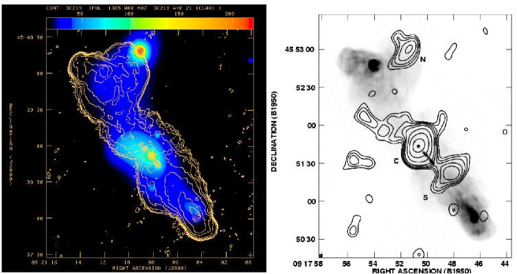
Figure 9.  : Panel a: Radio VLA contours at 1.4 GHz of 3C 219 superimposed on the Chandra 0.3–8 keV image (grays). The X–ray image is smoothed after removal of the nuclear source which affects only the innermost 3-5 arcsec. Panel b: X–ray ROSAT HRI image (contours) obtained after the subtraction of the nuclear source is overlaid with a VLA radio image (grays). The subtraction of the X–ray nucleus strongly affects the X–ray contours in the innermost 20 arcsec.

Diffuse emission coincident with the radio lobes also showing a brightness increment in the innermost part of the northern lobe is clearly detected.

The combined imaging and spectral analysis of this emission ($\sim 400$ net counts) point to a non–thermal, IC/CMB origin of the large scale diffuse emission. Following the procedure described in Section 3.5.2, the comparison between radio and X–ray IC emission yields a precise measurement of the magnetic field intensity (averaged over the total radio volume) which results a factor of $\simeq 2.9$ times lower than the equipartition value (assuming $\gamma_{\rm low}=50$ in Eq.(38). Under these conditions, the ratio between particle and field energy densities (Sect.3.5.2) is $\simeq 64$. The derived energetics of the lobes of 3C 219 is $\simeq 10^{60}$erg which results a factor $\simeq 7$ larger than that estimated with classical equipartition formulae (Sect.3.5.1). The bulk of the energy density of the radio lobes is associated to the electrons with $\gamma<500$.

The increment in the X–ray brightness present in the innermost part ($\sim 70$ kpc) of the northern lobe (counter lobe) may indicate an additional contribution due to IC scattering of nuclear photons, thus providing direct evidence for the presence of $\gamma\sim 10^{2}$ electrons in the lobes. Finally, two distinct knots at 10–25 arcsec south of the nucleus, spatially coincident with the radio knots of the main jet, are visible in the Chandra image.

Past combined ROSAT PSPC, HRI and ASCA observations did also find evidence for IC emission in 3C 219 lobes out of equipartition conditions (Brunetti et al. 1999). However, the presence of the strong nuclear source, the impossibility to perform spatially resolved spectroscopy and the relatively poor sensitivity of ROSAT HRI required a follow up observation with Chandra. The 0.1–2 keV image from the 30 ksec ROSAT HRI observation is shown in Fig.9b: the emission within $\sim 20$ arcsec from the nucleus is strongly affected by the subtraction of the nuclear source. The comparison of the two images in Fig.9 is very instructive and shows well the real breakthrough in X–ray imaging provided by Chandra.

4.2 X–ray observation of IC scattering of nuclear photons from radio lobes

The detection of X–ray emission from IC/QSO has been recently achieved in at least three objects (3C 179, 3C 207, 3C 295) whereas possible evidences have been suggested in other few cases (e.g., 3C 294: Fabian et al. 2001; 3C 219, Fig.9). A positive detection of this effect with Chandra was a specific prediction of this model in the case that a substantial fraction of the energetics of the radio lobes is associated to the low energy end of the electron spectrum. X–ray emission from IC scattering of nuclear photons with the relativistic electrons in the radio lobes is expected to be particularly efficient in the case of relatively compact (i.e., $\leq 100$ kpc) and strong FRII radio galaxies and steep spectrum radio quasars. This is due to the dilution of the nuclear flux with distance from the nucleus.

Radio galaxies: 3C 295

This is a classical FRII at the center of a rich cluster (z=0.461). The X-ray data obtained with previous instruments (Einstein Observatory: Henry & Henriksen 1986; ASCA: Mushotzky & Scharf 1997; ROSAT: Neumann 1999) only allowed the study of the cluster emission.

3C 295 was the first FRII source observed by Chandra. Harris et al. (2000) obtained the 0.3–7 keV image of this radio galaxy in which the hot spots and nuclear emission were well separated from the surrounding cluster contribution. The presence of possible diffuse X–ray emission related to the radio lobes was first addressed by these authors. However, the morphology and intensity of this emission resulted particularly uncertain due to the presence of the bright nuclear source and of the northern hot spot at $\sim 2$ arcsec distance. Stimulated by the results of Harris et al. (2000), Brunetti et al. (2001b) performed a more detailed analysis in order to maximize the information on the X–rays from the radio lobes.

In particular, these authors performed the spectrum of the nuclear source which cames out to be highly absorbed by a column density of $\sim 10^{23}$cm^-2 and thus almost absent in the 0.2–2 keV image. This image is shown in Fig.10:

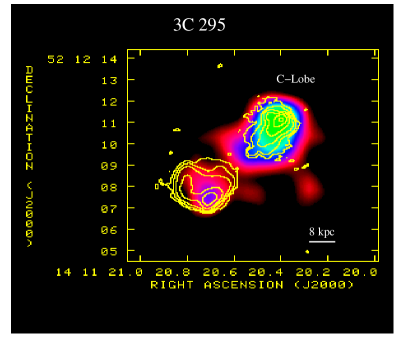
Figure 10.  : The GHz VLA radio map (contours) of 3C 295 is shown superimposed on the 0.1–2 keV Chandra image (grays). The X–ray image is obtained after the subtraction of the cluster emission.

the morphology of the diffuse X–ray emission is double lobed with the X–rays coincident with the radio lobes, thus pointing to a non–thermal origin. In addition the asymmetry in the X–ray brightness (with the northern lobe a factor $\sim 2-4$ brighter than the southern one) appears to be the signature of the IC/QSO model. In order to reproduce the observed brightness ratio with this model an angle between radio axis and the plane of the sky of 6–13^o is required with the northern lobe being further away from us. This geometry was confirmed by the discovery of a faint radio jet in the southern lobe (i.e., the near one) by P.Leahy with a deep MERLIN observation (private communication).

As stated in Sect.3, the spectrum from IC scattering of nuclear photons is a unique tool to constrain the energy distribution of $\gamma\sim 100-300$ electrons.

Figure 11.  : The 0.5–2 keV spectral index expected in the case of the IC scattering of nuclear photons is reported in the case of 3C 295. In the calculation we have assumed the Sanders et al. (1989) (solid lines) average SED of quasars and the SED of 3C 48 (dashed lines). For each SED we have reported two different curves giving uncertainties on the spectral index due to different set of parameters assumed in the model calculation. The limits on the observed 0.5–2 keV spectral index from our Chandra data analysis are also reported (dotted lines).

Fig.11 shows the 0.5–2 keV spectral index predicted by the model as a function of a low energy cut–off in the electron spectrum : an upper limit $\gamma_{\rm low}<100$ is obtained from the Chandra data.

The IC scattering of the nuclear photons has been also used to calculate the magnetic field strength in the lobes of 3C 295. ISO measurement of 3C 295 flux (Meisenheimer et al. 2001) fix the far–IR nuclear luminosity to $\sim 3\times 10^{46}$erg s^-1 and the deriving value of the IC magnetic field strength results consistent with the value calculated under minimum energy assumption (Fig.12). The derived energetics of the radio lobes of 3C 295 is $\simeq 4.4\times 10^{59}$erg and results a factor $\sim 2$ larger than that derived with classical equipartition formulae (Sect.3.5.1); a significant fraction of it is associated to the $\gamma\leq 300$ electrons.

Figure 12.  : The ratio between the equipartition magnetic field intensity ($B_{\rm eq}$) and that estimated from the IC scattering is reported as a function of the low energy cut–off $\gamma_{\rm low}$. The calculation are performed for a bolometric far–IR/optical luminosity of the hidden quasar = 2–4$\times 10^{46}$erg s^-1; k is the ratio between proton and electron energy density in the radio lobes.

Lobe dominated quasars: 3C 179 and 3C 207

The effect of the asymmetry in the X–ray distribution from the anisotropic IC scattering of the nuclear photons is maximized in the case of the steep spectrum quasars, which typically make an angle of 10–30 degrees between the radio axis and the line of sight. This provides an unambiguous identification of the process responsible for the X–ray emission as only the X–rays from the counter lobe are expected to be efficiently amplified and thus detected. In addition, in this case the far–IR to optical flux from the nuclear photons can be directly measured thus allowing a prompt estimate of the energy density of the scattering electrons (and magnetic field) in the radio lobes as in the case of the IC scattering of CMB photons (Sect.3.5.2).

So far there are two radio loud quasars observed with Chandra in which extended X–ray emission from the counter–lobe has been successfully detected, and for which no diffuse emission from the near lobe was detected: 3C 179 (Sambruna et al. 2002) and 3C 207 (Brunetti et al. 2002b). Both these sources are relatively compact and luminous, with prominent radio lobes making them ideal candidates to detect IC scattering of the nuclear photons in the radio lobes.

The 0.2–8 keV images of 3C 207 ($\sim$ 36 ksec exposure) is reported in Fig.13 superimposed on the VLA radio contours.

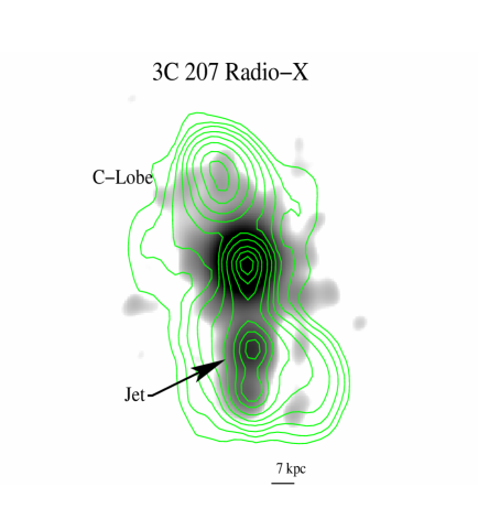
Figure 13.  : Chandra 0.2–8 keV image of 3C 207 (grays) superimposed on the 1.4 GHz VLA contours. The X–ray jet and counter lobe are indicated in the figure. The scale bar gives the resolution of the X–ray image (0.9 arcsec = 7 kpc); the resolution of the radio image is 1.4 arcsec.

Figure 14.  : The allowance regions for the ratio between IC–magnetic field and equipartition field strength and for $\gamma_{\rm low}$ in the case of 3C 207 are reported for different assumed energy distributions of the electrons: power law $\delta=2.8$ down to $\gamma_{\rm low}$ (thick solid region), accelerated spectrum with $\gamma_{*}/\gamma_{\rm low}$=2 (dashed region) and =50 (thin solid region). In the case of reaccelerated electron spectra, the regions are calculated by assuming $\gamma_{\rm b}$ in the range 500–1000 and $\gamma_{c}>>1000$.

The allowed regions of the values of the magnetic field strengths and of $\gamma_{\rm low}$ (Sect. 3.3) as inferred by the combined radio and X–ray fluxes and spectrum of 3C 207 are reported in Fig.14: the magnetic field strengths are lower, but within a factor of $\sim 2$, from the equipartition values. The resulting energetics of the radio lobes of 3C 207 is $\simeq 3\times 10^{60}$erg; a large fraction of it is associated to the $\gamma\leq 300$ electrons. The above value of the energetics is a factor $\sim 4.5$ larger than that obtained for 3C 207 with classical minimum energy formulae (Sect. 3.5.1). The shorter Chandra exposure ($\sim$ 9 ksec) in the case of 3C 179 makes difficult to constrain the energetics of the radio lobes. However, also in this case, the detection of IC/QSO proves that a consistent fraction of the energetics of the electrons component in the radio lobes is associated to low $\gamma$ electrons.

4.3 Jets and hot spots

RADIO OBSERVATIONS: Radio telescopes have imaged a large number of jets and hot spots of radio sources with arcsec or subarcsec spatial resolution (e.g., T.Venturi, this proceeding). The radio studies suggested the basic modelling of radio jets and hot spots. They provided evidence for relativistic motions of the radio jets from pc to kpc distances from the nucleus (e.g., Garrington et al. 1988; Bridle et al. 1994). The study of the polarization from jets and hot spots have suggested the presence of shocks and/or strong interactions with the surrounding IGM/ICM in which magnetic field amplification and particle reacceleration can take place. Finally, the study of the spectral synchrotron ages, combined with the direct (or statistical) measurement of the advancing motion of the radio lobes/hot spots have allowed a first order estimate of the dynamical age of extragalactic radio sources. This in turn allowed the measurement of the jet kinetic power under the assumption of minimum energy conditions (Rawlings & Saunders 1991).

Although the improvement of the radio telescopes and interferometers, and the advent of the future radio instruments (e.g., SKA) will allow to address a number of additional/substantial improvements in our understanding of the physics of radio sources, a multiwavelength approach is by far the most efficient tool to provide the next step in this topic. This is due to the synchrotron degeneracy (Sect.3.5.1).

OPTICAL OBSERVATIONS: although the search for optical emission from radio jets and hot spots has a long history (e.g., Saslaw et al. 1978; Simkin 1978; Crane et al. 1983), relatively few jets and hot spots have been detected as sources of optical emission so far (Tab.2, Tab.3, Meisenheimer et al. 1997). This is not only due to the power law decay with frequency of the synchrotron spectrum emitted from these regions, but also due to the presence of breaks and/or exponential cut-offs in the synchrotron spectrum below the optical band (Sect.3.3). The advent of the Hubble Space Telescope (HST) and more recently, of the 10 mt. generation of ground based telescopes (e.g., VLT, Gemini), has considerably improved the possibility to detect and study the optical emission from these regions.

X–RAY OBSERVATIONS: the study of X–ray emission from jets and hot spots has been considerably improved by the recent advent of the Chandra observatory. Before Chandra only a few cases of X–ray counterparts of radio jets and hot spots was discovered (see Tab. 2 and 3). The most spectacular result being the famous ROSAT HRI detection of both hot spots of the powerful radio galaxy Cygnus A (Harris et al. 1994). It was immediately clear from these past observations that the detected emission was of non–thermal origin with the best interpretation provided by synchrotron and SSC mechanisms under approximate minimum energy conditions. Likewise Chandra is really providing a significant progress on the study of the X–ray emission from jets and hot spots (see Tab. 2 and 3). Although the analysis of the increasing number of successful detections of X–ray emission from compact hot spots and jets has unambiguously confirmed the non–thermal nature of the X–rays from these sources, it is not clear whether the SSC and synchrotron model can provide or not a general interpretation of the data (e.g. Harris 2001). In addition the possibility to derive spectral analysis of the X–ray counterparts allows, for the first time, to constrain the spectrum of the emitting electrons in these regions.

In this Section we especially focus on the information on the low energy end and high energy end of the electron spectrum which are becoming available with the most recent multiwavelength studies.

Constraining the LOW energy end of the electron spectrum

As discussed in Sect.3.4, information on the low energy end of the electron spectrum can be provided by the detection of optical SSC fluxes from the hot spots and by the detection of X–ray emission via IC/CMB from the jets.

a) Optical SSC emission from hot spots – 3C 295–N and 196–N – : The northern hot spot of 3C 295 has been recently detected in the B–band with the HST telescope (Harris et al. 2000). Taking into account the radio, optical and X–ray data, Brunetti (2000) has shown that the radio to optical emission is not easily accounted for by a simple synchrotron model, whereas a synchrotron plus SSC model can account very well for the broad band spectrum with the radio matched by the synchrotron radiation, and the optical and X–rays matched by the SSC (Fig.15).

Figure 15.  : The radio to X–ray data points of the northern hot spots of 3C 295 are fitted with a synchrotron and SSC model: the SSC accounts for both optical and X–ray data.

The synchrotron radiation at $\geq$ GHz frequency is emitted by $\gamma>1000$ electrons (Sect.3.4), whereas the SSC optical radiation is emitted by $\gamma\sim 500$ electrons. In particular, the model in Fig.15 is calculated assuming that the spectrum of the synchrotron emitting electrons can be extrapolated at lower energies ($\gamma_{\rm low}<500$) and the data constrained the low energy break in the electron spectrum (if any) at $\gamma_{*}<800$ (Sect. 3.3).

The optical counterpart of the northern hot spot of 3C 196 has been recently discovered by Hardcastle (2001) with the HST telescope. The high frequency radio fluxes show a prominent steepening so that a synchrotron model accounting for the radio spectrum is too steep and falls well below the optical flux. As in the case of 3C 295-N, a viable explanation for the optical emission is provided by the SSC mechanism under the assumption of approximate equipartition conditions in the hot spots (Hardcastle 2001). As in the case of 3C 295, the detection of optical SSC emission from the hot spot of 3C 196 points to the presence of $\gamma\sim 500$ electrons in the hot spot volume without a significant flattening of the electron spectrum at these energies.

TABLE 2.  : High power objects

  Name z Type Assoc. Assoc. Chandra Reference Radio Optical  3C 123 0.2177 RG HS N Y Ha01 Pictor A 0.0350 RG HS Y N W01 Knots N Y PKS 0637-752 0.653 FSQ Knots Y Y C00,T00,Sc00,Ce01 3C 179 0.846 FSQ Knot N Y S02 HS N Y 3C 207 0.684 FSQ Knot N Y B02b HS N Y Q 0957+561 1.41 FSQ Knots N Y C02 PKS 1127-145 1.187 FSQ Knots N Y Si02 PKS 1136-135 0.554 FSQ Knots Y Y S02 4C 49.22 0.334 FSQ Knots Y Y S02 3C 273 0.1583 FSQ Knots Y N M01,S01 4C 19.44 0.720 FSQ Knots Y Y S02 3C 295 0.45 RG HS Y Y H00,B01b 3C 351 0.3721 SSQ HS Y Y B01c 3C 390.3 0.0561 RG HS Y N P97,H98 Cyg A 0.0560 RG HS N N H94,W00   

References: Ha01=Hardcastle et al. 2001a, W01=Wilson et al. 2001, C00=Chartas et al. 2000, T00=Tavecchio et al. 2000, Sc00=Schwartz et al. 2000, Ce01=Celotti et al. 2001, S01=Sambruna et al. 2002, B02b=Brunetti et al. 2002b, C02=Chartas et al. 2002, Si02=Siemiginowska et al. 2002, M01=Marshall et al. 2001, S01=Sambruna et al. 2001, H00=Harris et al. 2000, B01b=Brunetti et al. 2001b, B01c=Brunetti et al. 2001c, P97=Prieto 1997, H98=Harris et al. 1998, H94=Harris et al. 1994, W00=Wilson et al. 2000. See http://hea-www.harvard.edu/XJET/index.html for an updated list.

b) X–ray emission from radio jets – external IC scattering –: one of the most impressive results from Chandra is the unexpected high detection rate of the radio jets in the powerful radio sources (Tab.2). The first object with a prominent X–ray jet discovered by Chandra was the flat spectrum quasar PKS 0637-752 at a redshift of z=0.653 (Chartas et al. 2000; Schwartz et al. 2000). The combined radio, optical and X–ray data exclude the possibility of synchrotron X–ray emission. In addition Tavecchio et al.(2000) and Celotti et al.(2001) have shown that an SSC origin of the X–rays should require huge departures from equipartition, and an extremely high kinetic power of the jet. These authors were the first to successfully make use of the IC scattering of CMB photons by the relativistic electrons of the jet (a mechanism previously considered only for the jets on pc scales, e.g., Schlickeiser 1996) to reproduce the X–ray data of this object. In order to successfully fit the X–ray spectrum with this model they derive a high relativistic velocity ($\Gamma_{\rm bulk}\sim 10$) of the jet up to hundreds of kpc distance from the nucleus. In order to maintain such velocities, small radiative efficiencies in the jets are required with most of the energy extracted from the central black hole stored in the bulk motion of the plasma. In addition, as pointed out by Ghisellini & Celotti (2001), it can be considered that the radiative efficiency of the jet decreases with increasing the jet luminosity.

Additional evidences in favour of the IC/CMB and thus that high relativistic velocities are maintained by the jets up to tens or hundreds of kpc from the nucleus, is coming from other objects (e.g., Sambruna et al. 2002; Tab.2). In Fig.16a-c we report a compilation of radio to X–ray spectral energy distributions of some of these objects.

Figure 16.  : A compilation of SEDs of X–ray jets fitted with synchrotron and IC models. Panel a)–c): SEDs in the case of jets of high power radio objects. Radio and optical data are fitted with synchrotron models, while X–ray data are accounted for via IC/CMB models. The SSC predictions are also reported in the case of 3C 207 (Panel b). Panel d)–f): SEDs in the case of jets of low power radio objects. Radio, optical and X–ray data can be fitted with a synchrotron model which includes a non standard electron transport or adiabatic losses in the post–shock region. Standard synchrotron models (e.g., dotted line in 3C 66B, upper curves in PKS 0521-365 and B2 0755+37) cannot well account for the data.

One of the most striking cases is the X–ray knot of the quasar 3C 207 at a redshift z=0.684 (Brunetti et al. 2002b). The resulting X–ray spectrum is considerably harder than the radio spectrum ($\Delta\alpha\sim 0.6$) so that it cannot be reproduced by the SSC spectrum even releasing the assumption of minimum energy conditions in the jet. On the other hand, as discussed in Sect.3.3, the electron spectrum of the low energy electrons emitting X–rays via IC/CMB ($\gamma\sim 100$) might be harder than that of the higher energy radio synchrotron electrons ($\gamma>1000$), thus providing a natural explanation for the difference between X–ray and radio spectrum of this knot. It should be noted that, despite the poor statistics, a similar difference between radio and X–ray spectrum is also found in the jet of PKS 1127-145, which is the most luminous IC/CMB jet discovered so far (Siemiginowska et al. 2002).

If the IC/CMB interpretation is correct for these X–ray jets, then, for the first time, the modelling of the radio to X–ray spectrum allows the low energy end of the electron spectrum to be constrained in the regions where these electrons are (re)accelerated. These studies, however, are relatively complicated as the energy of the electrons giving the observed X–rays (Sect.3.4) depends on both the Lorentz factor of the bulk motion, and on the angle between the jet velocity and the line of sight. In the case of 3C 207 it can be shown that for substantial boosting (i.e., $\Gamma_{\rm bulk}>4$ and $\theta<10^{o}$) $\gamma_{\rm low}$$<$ $\sim$50$\leq\gamma_{*}$, whereas in the case of PKS 0637-752 $\gamma_{\rm low}$$<$ $\sim$30.

Constraining the HIGH energy end of the electron spectrum

a) synchrotron optical emission from radio hot spots: As already discussed in Sect.3.4, synchrotron optical emission from radio hot spots is mainly due to $\gamma\geq 10^{5}$ electrons, which are probably close to the high energy end of the spectrum of the electrons accelerated in these regions. These electrons have a radiative life time about 300 times shorther than that of the electrons emitting the synchrotron radio spectrum of the same hot spots. Hence the optical detection of hot spots generally implies the in situ production of such energetic electrons (e.g., Meisenheimer et al., 1989). An important confirmation that the optical emission from the hot spots is of synchrotron nature is provided by the detection of optical linear polarization in a number of cases (3C 33: Meisenheimer & Röser, 1986; 3C 111, 303, 351, 390.3: Lahteenmaki & Valtaoja 1999; Pictor A West: Thomson et al. 1995). So far there are only about 15 hot spots detected in the optical band (see Gopal-Krishna et al. 2001 and ref. therein) and the radio to optical spectrum of these hot spots is well fitted by synchrotron radiation emitted by electrons accelerated in a shock region (e.g., Meisenheimer et al. 1997). In Fig.17 we report the radio to optical data of a few representative cases fitted with synchrotron models.

In principle, if this scenario is correct, the theory of shock acceleration allows us to get an independent estimate of the field strength at the hot spot by measuring the break and cut–off frequencies of the synchrotron spectrum and the hot spot length (e.g., Meisenheimer et al., 1989). This allows the estimate of both the maximum energy of the emitting electrons, and of the acceleration efficiency of the shock. In general, the estimated magnetic field strength is consistent with that estimated under minimum energy conditions within a factor of 2–3 (e.g., Meisenheimer et al., 1997). With these values, we have that the Lorentz factors of the electrons at the cut–off is in the range $\gamma_{\rm c}=10^{5}-10^{6}$, and that the acceleration time in the shock region is in the range $\sim 10^{2}-10^{3}$yrs.

Figure 17.  : Synchrotron fits to the radio – optical SEDs of the radio hot spots 3C 20 East and West are reported. The spectrum of the emitting electrons is calculated under shock acceleration assumptions (Sect.3.3, Figs.3-4). In the case of 3C 20 West the values of the break and cut–off frequency are also given. The expected X–ray emission from both the hot spots due to SSC process are reported under equipartition conditions (lower curves) and assuming a magnetic field 2 times smaller than the equipartition (higher curves).

An alternative scenario to that of the shock acceleration might be an extremely efficient transport – minimum energy losses – of the ultra relativistic electrons all the way from the core to the hot spots (e.g., Kundt & Gopal-Krishna 1980). Based on the evidences for relativistic jet bulk motion out to 100–kpc scales, Gopal-Krishna et al. (2001) have recently reconsidered a minimum loss scenario in which the relativistic electrons, accelerated in the central active nucleus, flow along the jets losing energy only due to the inescapable IC scattering of CMB photons. Under these assumptions, comparing the electron radiative life time with the travel time to the hot spots, these authors find that in situ electron re–acceleration is in general not absolutely necessary to explain the optical synchrotron radiation from the hot spots. In the framework of this minimum loss scenario, in Fig.18 we report the maximum distance that synchrotron optical electrons can cover as a function of the velocity of the jet flow, and for two different magnetic field strengths in the hot spot region.

Figure 18.  : The maximum distance (projected on the plane of the sky) that electrons emitting synchrotron radiation at $\nu=5\cdot 10^{14}$Hz can cover is reported as a function of the velocity (v/c) of the jet. The calculation are performed for different inclination angles of the jet: quasar–like (solid lines) and radio galaxy–like (dashed lines). The results are shown in the case of z=0.2 (thin lines) and z=0.5 (thick lines).

Such distance is in general less than 100 kpc except in the case in which the magnetic field strength in the hot spot is very large. On the other hand, a number of optically detected radio hot spots are found at larger distances from the nucleus. In addition, the double hot spot in 3C 351 represents a clear counter example to the minimum energy loss scenario. Indeed, in this case the hot spot magnetic field ($B\leq 100\mu$G) is constrained matching the X–ray flux by the SSC process, and the distance of the hot spots from the nucleus is $>180$ kpc. As both the hot spots emit synchrotron radiation at optical wavelengths, in situ reacceleration appears to be inescapable (Brunetti et al. 2001c).

b) synchrotron X–ray emission from jets: One of the most interesting findings of Chandra is that X–ray jets are relatively common also in the case of low power radio sources (Worral et al., 2001). These X–ray jets are usually interpreted as synchrotron emission from the very high energy end ($\gamma\sim 10^{7}$) of the electron population. Such interpretation is mainly supported by the observed radio to X–ray spectral distributions. In addition, it is supported by the fact that, contrary to the case of high power radio sources, the jets of low power objects are believed to move at sub/trans–relativistic speeds at kpc distances from the nucleus (e.g., T.Venturi, this proceedings and ref. therein) and thus the X–ray emission from IC/CMB is expected to be negligible. If so, the jets of low power radio sources can be considered laboratories to study the electron acceleration. Indeed, combining radio, optical and X–ray data it is possible to study the synchrotron spectrum from radio to X–ray frequencies and thus to sample the spectrum of the emitting electrons over more then 4 decades in energy. In particular, relatively deep multiwavelength observations with adequate frequency coverage of a few objects (M 87: Boehringer et al. 2001; 3C 66B: Hardcastle et al. 2001; PKS 0521-365: Birkinshaw et al. 2002) have shown that the radio to X–ray spectrum can be well fitted by a double power law model of slope $\alpha$ and $\alpha+(0.7-0.9)$ in the radio and in the optical to X–ray band, respectively. If further confirmed, this point is crucial as it generates problems in the interpretation of the data with acceleration models including standard electron diffusion in the post shock region (e.g. Bell, 1978a,b; Heavens & Meisenheimer, 1987) which, indeed, would predict a steepening of the synchrotron spectrum of only 0.5 in the optical to X–ray band.

More recently Dermer & Atoyan (2002) have proposed that synchrotron emission can successfully fits the X–ray data also in the case of some of the detected X–ray jets of high power radio sources usually interpreted via IC/CMB scattering. These authors have investigated the evolution of the spectrum of electrons accelerated up to very high energies ($\gamma>10^{8}$) under the hypothesis that the radiative losses of the electrons are largely dominated by IC scattering rather than synchrotron. Under these conditions, if the photon energy density in the jet frame is dominated by boosted CMB photons (as in the case of the IC/CMB process), the energy dependence of the IC losses of the electrons with $\gamma>10^{7}$ changes due to the effect of the Klein–Nishina cross section and the radiative losses for these electrons result alleviated (Fig.1). It can be shown that, under these conditions, the spectrum of the electrons may become harder for $\gamma>10^{7}$ and that the resulting synchrotron emission may present a bump in the X–ray band similarly to that observed by Chandra. Assuming a transverse velocity structure in the jets, with a fast central spine surrounded with a boundary layer with a velocity shear (Sect. 4.3.5), it has been proposed that turbulence may also accelerate high energy electrons at such boundary layers (Owstroski, 2000; Stawarz & Ostrowski, 2002a). If this happens, X–ray synchrotron radiation from large scale jets is expected and it may account for some of the observed Chandra jets (Stawarz & Ostrowski, 2002b).

c) synchrotron X–ray emission from hot spots ?:

The effect of electron radiative cooling and the presence of a high energy cut–off in the electron spectrum produce an abrupt steepening of the spectrum of the hot spots below that extrapolated from the lower frequency power–low. This makes X–ray detection of synchrotron emission very difficult. In addition the photons emitted by competing processes particularly efficient at high frequencies (e.g., SSC) might completely hide those contributed by the synchrotron emission. So far, there are only two relatively secure cases of hot spots in which the synchrotron spectrum is given by a power law from the radio to the UV or even X–rays (3C 303 : Keel 1988, Meisenheimer et al. 1997 ; 3C 390.3 : Prieto 1997, Harris et al. 1998), indicating the continuation of the synchrotron spectrum at higher frequencies. An immediate implication is the presence of relativistic electrons with $\gamma\geq 10^{7}$ which, due to their short life time (considering typical hot spots’ magnetic field strength $\geq 100\mu$G), require very efficient acceleration processes (acceleration time $\leq 100$ yrs) and/or magnetic field strengths in the acceleration regions well below that calculated under equipartition conditions.

Energetics: X–ray SSC emission from radio hot spots in FR II

Until the advent of Chandra clear evidence for SSC emission had only been detected in the case of the hot spots of Cygnus A (Harris et al., 1994) in which case the magnetic field results close to the equipartition value.

Chandra has enabled significant progress in this field, with a number of successful detections in the first three years of observations (3C 295: Harris et al. 2000; Cyg A: Wilson et al. 2000; Pictor A: Wilson et al. 2001; 3C 123: Hardcastle et al. 2001; 3C 351: Brunetti et al. 2001c).

In the majority of the detected hot spots (Cygnus A–W and E, 3C 295–N, 3C 123) the magnetic fields derived comparing the radio and X–ray fluxes (Sect.3.5.2) result within a factor of 2 from the equipartition value. This has further motivated the usually adopted assumption of approximate equipartition between magnetic field and electron energy densities.

On the other hand, in the case of the double northern hot spots of 3C 351 (J and L components), if the SSC interpretation is correct, the magnetic field would result in both cases from a factor 3.5 to 5 smaller than the equipartition value (in case of ordered or isotropic field configuration, respectively). Here we stress that this departure from equipartition implies an energy density of the electrons in the hot spots a factor $>60$ larger than that of the magnetic field. Such a relatively strong departure from equipartition in these hot spots is further suggested by the modelling of the broad band synchrotron spectrum (Fig.19). Indeed, the magnetic field intensity, derived combining the optical synchrotron cut–off and break frequencies with the hot spots’ lengths along the jet direction, lead to an independent estimate of the magnetic field strengths which is in good agreement with those obtained with the SSC argument (Brunetti et al. 2001c).

Figure 19.  : The radio, optical and X–ray data of the hot spots 3C 351–J (left panel) and 3C 351–L (right panel) are reported together with the synchrotron and SSC spectra. The spectrum of the emitting electrons is calculated assuming shock acceleration (Sect.3.3, Figs.3-4). Radio and optical fluxes are accounted for by synchrotron emission, whereas the X–rays are matched via SSC. In both cases, the reported SSC models are calculated assuming a substantial departure from equipartition conditions (see text for details).

A particular intriguing case is the west hot spot of Pictor A (Wilson et al. 2001). The synchrotron spectrum shows an abrupt cut–off clearly indicated by a large number of optical data points and it falls orders of magnitude below the X–ray flux. On the other hand, the SSC interpretation would require a magnetic field strength about a factor 14 below the equipartition value to match the observed X–ray flux. In addition, the Chandra X–ray spectrum of the hot spot is relatively steep ($\alpha\simeq 1.1$) and it is poorly fitted by the spectrum expected in case of SSC emission ($\alpha\simeq 0.74$).

TABLE 3.  : Low power objects

  Name z Type Assoc. Assoc. Chandra Reference Radio Optical  3C 31 0.0167 RG Knots N Y Ha02 B2 0206+35 0.0368 RG Knots N Y Wo01 3C 66B 0.0215 RG Knots Y Y Ha01 3C 120 0.0330 RG Knot N N H99 B2 0755+37 0.0428 RG Knots Y N Wo01 3C 270 0.00737 RG Knots Y? Y Ch02 M 87 0.00427 RG Knots Y N Bi91,M02,W02 Cen A 0.001825 RG Knots ? Y F91,K02 3C 371 0.051 BL Knots Y Y P01   

References: Ha02=Hardcastle et al. 2002, Wo01=Worrall et al. 2001, Ha01=Hardcastle et al. 2001b, H99=Harris et al. 1999, Ch02=Chiaberge et al. 2002, Bi91=Biretta et al. 1991, M02=Marshall et al. 2002, W02=Wilson & Yang 2002, F91=Feigelson et al. 1991, K02=Kraft et al. 2002, P01=Pesce et al. 2001. See also http://hea-www.harvard.edu/XJET/index.html for an updated list.

Multiple electron populations in jets and hot spots ? : Pic A west and 3C 273 jet

One possibility to match the radio, optical and X–ray data of Pictor A west is to have two electron populations (Wilson et al. 2001). The first population of electrons (with injection spectral index $\delta\simeq 2.5$) is assumed to be in a region of relatively strong magnetic field (e.g. of the order of the equipartition field) and would be the responsible for the observed radio to optical spectrum via synchrotron emission. As already noticed, such a population would produce a SSC emission about two orders of magnitude below the observed X–ray flux. Thus it might be assumed a second population of relativistic electrons in the hot spot (with injection spectral index $\delta\simeq 3.3$), spatially separated from the first population and in low field regions. This second population would emit negligible synchrotron radiation and it may produce efficient IC scattering of the synchrotron radio–optical photons (from the first population) matching the observed X–ray spectrum. Alternatively, the electron spectrum of the second population might extend up to very high energies (with $\nu_{\rm c}>10^{17}$Hz) matching the X–rays via synchrotron radiation. In this last case a value of the injection spectral index $\delta\simeq 2.15$ and a break frequency in between $10^{11}$ and $10^{17}$Hz is required in order to not overproduce the synchrotron spectrum emitted by the first population (Wilson et al. 2001). Both these possibilities are ad hoc and, so far, they are not well physically motivated so that the case of Pictor A west remains poorly understood and future radio and Chandra observations are still required.

A second interesting case of possible multiple electron populations is the well studied jet of 3C 273. Recently, Marshall et al.(2001) and Sambruna et al.(2001) performed a detailed radio, optical (HST) and X–ray (Chandra) study of this jet. These authors provide different interpretations of the stronger knots in this jet. In particular, Sambruna et al.(2001) have suggested an IC/CMB interpretation for the X–ray spectrum of the knots since a synchrotron model from a single electron population cannot fit the radio to X–ray spectra. On the other hand, making use of a different data set, Marshall et al.(2001) were able to fit the observed spectra with a single synchrotron model. The most important difference in the two data sets is given by the different slopes of the optical spectra; additional observations and more detailed data analysis are probably requested to understand this discrepancy. A detailed optical–UV study of the jet of 3C 273 has been performed by Jester et al.(2001). These authors have measured the optical–UV spectral index along the jet discovering that it is only slowly changing without showing a clear trend along the jet. This has been interpreted as the signature of continuous reacceleration processes (Fermi I and II – like) of the relativistic electrons active along the jet which, in principle, might yield multiple electron populations or a single electron population with a complex spectrum. It should be noticed that, indeed, Sambruna et al.(2001) do not exclude the possibility to fit the radio to X–ray spectrum of the knots with synchrotron emission by ad hoc multiple (or complex) electron populations. A further step forward in the study of the jet of 3C 273 has been recently obtained by Jetser et al.(2002). These authors discovered the presence of an UV excess in the bright knots with respect to that expected from standard synchrotron models. This strengthens the possibility of a complex spectrum of the electrons or the presence of coexisting multiple electron populations. Jester et al.(2002) have also pointed out that the UV excess in the knots A and D2+H3 is consistent with the contribution due to the extrapolation at UV frequencies of the X–ray spectrum thus suggesting a common origin for the UV excess and for the X–rays. At the light of these results, we might conclude that the UV to X–ray spectrum can be produced by IC/CMB radiation emitted by the electron population giving the radio to optical emission via synchrotron process (as in Sambruna et al.2001). On the other hand, a synchrotron origin for the UV to X–ray spectrum of the bright knots cannot be excluded if a second - high energy - electron population is assumed (Jester et al. 2002). Additional multifrequency observations are required to test the different scenarios.

Velocity structure in radio jets

Komissarov (1990) suggested that the emission minima observed near the starting point of some FR I jets could result from Doppler dimming and that the appearance of the jet might be due to the presence of a slow moving boundary layer which would be less dimmed than the faster internal spine. Laing (1993) made the connection to polarization structure of FR I jets proposing a two component model consisting of an internal high velocity spine containing a magnetic field which has no longitudinal component but is otherwise random and a lower velocity external layer with an entirely longitudinal field structure. If FR I jets have field and velocity structure of this type and if they are launched at relativistic speeds decelerating away from the nucleus, the emission of the spine and layer components will suffer different effects due to beaming. Consequently, which component would dominate the emission properties of the jets depends on the angle with the line of sight and on the distance from the nucleus. This model provides a natural explanation for the tendency of the apparent magnetic field direction to be longitudinal close to the core and transverse further out. Detailed applications of models with velocity structure have been performed in the case of individual radio galaxies (e.g., 3C 31: Laing 1986; 3C 296: Hardcastle et al. 1997) and also for a small sub–sample selected from the B2 sample (Laing et al. 1999). More recently, Chiaberge et al.(2000) have explored the viability of the unification of BL Lacs and FR I radio galaxies by comparing the core emission of radio galaxies with those of BL Lacs of similar extended radio power in the radio-optical luminosity plane. In agreement with the Komissarov & Laing findings, these authors conclude that velocity structures in the jet are necessary to reconcile the observations with the unification scheme.

A possibility to study the velocity structure of radio jets (of both high and low power objects) on kpc scales is to compare their radio and X–ray emission properties. Assuming a transverse velocity structure, the emission of the jets pointing in the direction of the observer should be dominated by the contribution of the fast moving spine, whereas that from a misaligned jet should be dominated by the emission of the slow moving layer which is less dimmed by transverse Doppler boosting. In the case of high power radio objects, this scenario might be easily tested by Chandra. Indeed, these jets are highly collimated up to tens or hundreds kpc distance from the nucleus and thus indicating that their velocity structure (if any) should be preserved on large scales. As stated in Sect.4.3.1, the X–ray emission from the jets of core dominated quasars indicate a highly relativistic motion up to tens of kpc distance from the core. These velocities might be associated with a fast spine with a low radiative efficiency. On the other hand, future Chandra observations of the jets of the misaligned parent population (FR II radio galaxies) might constrain the contribution from any slow layer.

5 SUMMARY

In this contribution we have tried to summarize new insights on the physics of extragalactic radio sources from recent studies based on combined observations in different bands. We concentrated ourselves on the case of the non–thermal emission produced in kpc–scale regions (radio lobes, kpc–scale jets, hot spots) and on the spectrum and energetics of the emitting relativistic electrons.

We have shown that the spectrum of the relativistic electrons in radio sources can be approximated with a power law only in a relatively narrow energy range. In general, the shape of the spectrum depends on the acceleration mechanisms active in the emitting regions and on the competition between such mechanisms and both the processes responsible for the energy losses and the spatial diffusion of the relativistic electrons. Measurements of the flux and spectrum produced by different non–thermal emitting processes in different frequency bands can allow to trace the spectrum of the emitting electrons and thus to constrain the physics of the acceleration in these remote regions. Such measurements are possible only now by combining radio, optical and X–ray observations with arcsec resolution.

Here, a ‘biased’ summary of some of the most promising recent findings:

$\bullet$ Low energy end of the electron spectrum: An advance in constraining the energetics associated to the low energy electrons has coming from the new detections of extended X–ray emission from IC scattering of nuclear photons in powerful FR II radio galaxies and quasars. This effect opens a new window on the study of electrons with $\gamma\sim 100$ in radio lobes which are invisible in the radio band as, in general, they would emit synchrotron radiation in the 0.01 to 1 Mhz frequency range. We have stressed that, making use of the classical minimum energy formulae, these electrons are not taken into account in the calculation of the energetics of the radio lobes. On the other hand, the first X–ray detections of IC scattering of nuclear photons indicate that the bulk of the energetics of the radio lobes is contained by these low energy electrons. Additional evidences that the spectrum of the relativistic electrons extends down to low energies ($\gamma<500$) is provided by the possible detection of SSC optical emission from radio hot spots and by the X–ray emission from powerful radio jets due to boosted IC scattering of CMB photons.

$\bullet$ High energy end of the electron spectrum: The maximum energy of the electrons in extragalactic radio sources depends on the balance between acceleration and losses mechanisms. The discovery of optical synchrotron emission from hot spots in the last decades has pointed out the presence of efficient accelerators active in these regions and able to accelerate electrons up to very high energies ($\gamma\geq 10^{5}$). More recently, the discovery of synchrotron X–ray emission from an increasing number of jets of low power radio galaxies suggest the presence of even more energetic electrons ($\gamma\geq 10^{6-7}$) possibly accelerated in low B–field regions. These findings and the recent suggestion about synchrotron X–ray emission also from jets of powerful sources, would indicate the presence of extremely efficient accelerators in the emitting regions. The extremely short acceleration time–scales (down to $\sim 10^{2}$ yrs) requested by these findings are actually starting to put interesting limits on the spatial diffusion coefficient of the electrons and thus on the microphysics prevailing in these regions. The recent additional evidence for continuous reacceleration of relativistic electrons in radio jets might finally suggest the presence of energetic turbulence and thus that part of the kinetic power of the jets is dissipated into the developing of plasma instabilities and in the re–acceleration of relativistic particles. This might match with the proposed scenario in which a slow layer, where a fraction of the kinetic power is dissipated, surrounds a fast moving spine.

$\bullet$ Energetics of radio lobes and hot spots: A crucial point in the study of the extragalactic radio sources is the calculation of the energetics associated to these objects. As we have shown, the advent of Chandra makes it possible to extensively apply the IC method and to derive the energy density of the relativistic electrons and of the magnetic field in the emitting regions. This has been done in the case of a number of hot spots and radio lobes : the derived energetics are usually larger (1 to 30 times) than that calculated with the classical minimum energy formulae. This is a direct consequence of the presence of low energy electrons which contain most of the energetics, but it is also due to moderate departures from the minimum energy conditions found in a number of cases. Additional statistics is requested to better address this point. We further claim that deep X–ray follow up of the most unambiguous detections of diffuse IC emission from radio lobes will probably allow to derive the first maps of the magnetic field intensity in the extragalactic radio sources providing unvaluable information on the prevailing physics.

$\bullet$ Kinematics of the radio jets: One of the most interesting findings obtained combining the radio, optical and Chandra X–ray data of powerful radio jets is the recent discovery of highly relativistic speeds of the jets up to several tens of kpc of distance from the nucleus. Bulk Lorentz factors $\Gamma_{\rm bulk}\sim$ 3–10 up to these distances limit the radiative efficiency of the jets that should be low in order to preserve the kinetic power of the jet itself. Again, a scenario with a velocity structured jet with a fast spine surrounded by a slow layer might help to better understand this findings.

Acknowledgements I am grateful to all my collaborators, in particular to M. Bondi, A. Comastri and G. Setti for help and discussions. I am indebted to F. Mantovani who invited me to give these lectures and to M. Marcha for a careful reading of the manuscript and for useful comments.

References

- [] Aharonian, F.A., Atoyan, A.M., 1981, Ap&SS, 79, 321
- [] Arshakian, T.G., Longair, M.S., 2000, MNRAS, 311, 846
- [] Bell, A.R., 1978a, MNRAS, 182, 147
- [] Bell, A. R., 1978b, MNRAS, 182, 443
- [] Bicknell, G. V., Melrose, D. B., 1982, ApJ, 262, 511
- [] Birkinshaw, M., Worrall D. M., Hardcastle, M. J., 2002, MNRAS, in press; astro-ph/0204509
- [] Biretta, J. A., Stern C. P., Harris, D. E., 1991, AJ, 101, 1632
- [] Blandford, R. D., 1986, in Magnetospheric Phenomena in Astrophysics, eds. R.I. Epstein & W.C. Feldman (New York: AIP), p.1
- [] Blandford, R. D., Ostriker, J. P., 1978, ApJ, 221, L29
- [] Blandford, R. D., Eichler, D., 1987, Physics Rep., 154, 1
- [] Blasi, P., 2000, ApJ, 532, L9
- [] Blasi, P., 2001, APh, 15, 275
- [] Blumenthal, G. R., Gould, R. J., 1970, RvMP, 42, 237
- [] Böhringer, H., Belsole, E., Kennea, J., et al., 2001, A&A, 365, L181
- [] Borovsky, J. E., Eilek, J. A., 1986, ApJ, 308, 929
- [] Bridle, A. H., Perley, R. A., 1984, Ann. Rev. Astr. Ap., 22, 319
- [] Bridle, A. H., Hough, D. H., Lonsdale, C. J., Burns, J. O., Laing, R. A., 1994, AJ, 108, 766
- [] Brunetti, G., 2000, Astroparticle Physics, 13, 107
- [] Brunetti, G., Setti, G., Comastri, A., 1997, A & A, 325, 898
- [] Brunetti, G., Comastri, A., Setti, G., Feretti, L., 1999, A & A, 342, 57
- [] Brunetti, G., Setti, G., Feretti, L., Giovannini, G., 2001a, MNRAS, 320, 365
- [] Brunetti, G., Cappi, M., Setti, G., Feretti, L., Harris, D. E., 2001b, A & A, 372, 755
- [] Brunetti, G., Bondi, M., Comastri, A., et al., 2001c, ApJ, 561, L 157
- [] Brunetti, G., Comastri, A., Dallacasa, D., Bondi, M., Pedani, M, Setti, G. 2002a, Proc. Symposium New Visions of the X-ray Universe in the XMM-Newton and Chandra Era’; astro-ph/0202373
- [] Brunetti, G., Bondi, M., Comastri, A., Setti, G., 2002b, A & A, 381, 795
- [] Celotti, A., Ghisellini, G., Chiaberge, M., 2001, MNRAS, 321, L1
- [] Chartas, G., Worrall, D. M., Birkinshaw, M., et al., 2000, ApJ, 542, 655
- [] Chartas, G., Gupte V., Garmire G., et al., 2002, Apj, 565, 96
- [] Chiaberge M., Celotti, A., Capetti, A., Ghisellini, G., 2000, A&A, 358, 104
- [] Chiaberge M., Gilli, R., Macchetto, F. D., Sparks, W. B., Capetti, A., 2002, ApJ, submitted; astro-ph/0205156
- [] Clark, D. H., Caswell, J. L., 1976, MNRAS, 174, 267
- [] Cox, A. C., 1999, Allen’s Astrophysical Quantities (Springer-Verlag)
- [] Crane, P., Tyson, J. A., Saslaw, W. C., 1983, ApJ, 265, 681
- [] Daly, R. A., 1992, ApJ, 386, L9
- [] Dermer, C. D., 1995, ApJ, 446, L63
- [] Dermer, C. D., Atoyan, A. M., 2002, ApJ, 568, L81
- [] Dickel, J.R., 1983, in Supernova remnants and their X-ray emission, IAUS, 101, 213
- [] Eilek, J. A., Hughes, P. A., 1991, in Beams and Jets in Astrophysics, eds. P.A.Hughes (Cambridge astrophysics series), p.428
- [] Eilek, J. A., 1996, in Extragalactic radio sources, IAUS, 175, 483
- [] Eilek, J. A., Arendt, P. N., 1996, ApJ, 457, 150
- [] Fabian A. C., Crawford, C. S., Ettori, S., Sanders, J. S., 2001, MNRAS, 322, L11
- [] Feigelson, E. D., Schreier E. J., Delvaille J. P., et al., 1981, ApJ, 251, 31
- [] Feigelson, E. D., Laurent-Muehleisen, S. A., Kollgaard, R. I., Fomalont, E. B., 1995, ApJ, 449, L149
- [] Felten, J. E., Morrison, P., 1966, ApJ, 146, 686
- [] Feretti, L., Giovannini G., 1996, in Extragalactic radio sources, IAUS, 175, 333
- [] Ferrari, A., Trussoni, E., Zaninetti, L., 1979, A&A, 79, 190
- [] Garrington, S.T., Leahy, J. P., Conway, R. G., Laing, R. A., 1988, Nature, 331, 147
- [] Ghisellini, G., Celotti, A., 2001, MNRAS, 327, 739
- [] Ginzburg, V. L., 1969, Elementary Processes for Cosmic Ray Astrophysics (Gordon & Breach Science Publishers: New York)
- [] Gitti, M., Brunetti, G., Setti, G., 2001, A&A, 386, 456
- [] Gopal-Krishna, Subramanian, P., Wiita, P. J., Becker, P. A., 2001, A&A, 377, 827
- [] Gould, R. J., 1979, A&A, 76, 306
- [] Hamilton, R. J., Petrosian, V., 1992, ApJ, 398, 350
- [] Hardcastle, M. J., 2001, A & A, 373, 881
- [] Hardcastle, M. J., Alexander, P., Pooley, G. G., Riley, J. M., 1997, MNRAS, 288, L1
- [] Hardcastle, M. J., Worrall, D. M., 2000, MNRAS, 319, 562
- [] Hardcastle, M. J., Birkinshaw, M., Worrall, D. M., 2001a, MNRAS, 323, L 17
- [] Hardcastle, M. J., Birkinshaw, M., Worrall, D. M., 2001b, MNRAS, 326, 1499
- [] Hardcastle, M. J., Worrall, D. M., Birkinshaw, M., Laing R. A., Bridle A. H., 2002, MNRAS, in press; astro-ph/0203374
- [] Harris, D. E., 2001, in “Particles and Fields in Radio Galaxies”, R. A. Laing and K. M. Blundell (Eds.), ASP Conf. Series, in press; astro–ph/0012374
- [] Harris, D. E., Grindlay, J. E., 1979, MNRAS, 188, 25
- [] Harris, D. E., Stern, C. P., 1987, ApJ, 313, 136
- [] Harris, D. E., Carilli, C. L., Perley, R. A., 1994, Nature, 367, 713
- [] Harris, D. E., Leighly, K. M., Leahy, J. P., 1998, ApJ, 499, L 149
- [] Harris, D. E., Hjorth, J., Sadun, A. C., Silverman, J. D., Vestergaard, M., 1999, ApJ, 518, 213
- [] Harris, D. E., Nulsen, P. E. J., Ponman, T. J., et al., 2000, ApJ, 530, L 81
- [] Harris, D. E., Krawczynski, H., 2002, ApJ, 565, 244
- [] Heavens, A.F., Meisenheimer, K., 1987, MNRAS, 225, 335
- [] Henry, J. P., Henriksen, M. J., 1986, ApJ, 301, 689
- [] Jaffe, W. J., 1977, ApJ, 216, 212
- [] Jester, S., Röser, H.-J., Meisenheimer, K., Perley, R., Conway, R., 2001, A&A, 373, 447
- [] Jetser, S., Röser, H.-J., Meisenheimer, K., Perley, R., 2002, A&A, 385, L27
- [] Jones, T. W., O’Dell, S. L., Stein, W. A., 1974a, ApJ, 188, 253
- [] Jones, T. W., O’Dell, S. L., Stein, W. A., 1974b, ApJ, 192, 259
- [] Isenberg, P. A., 1987, JGR, 92, 1067
- [] Kaneda, H., Tashiro, M., Ikebe, Y., et al., 1995, ApJ, 453, L13
- [] Kardashev, N. S., 1962, Soviet Astronomy - AJ, 6, 3
- [] Katz–Stone, D. M., Rudnick L., 1997, ApJ, 488, 146
- [] Katz–Stone, D. M., Rudnick L., Butenhoff, C., O’Donoghue, A. A., 1999, ApJ, 516, 716
- [] Keel, W. C., 1988, ApJ, 329, 532
- [] Kirk, J. G., Rieger, F. M., Mastichiadis, A., 1998, A&A, 333, 452
- [] Kirk, J. G., Guthmann, A. W., Gallant, Y. A., Achterberg, A., 2000, ApJ, 542, 235
- [] Komissarov, S. S., 1990, Sov. Astronomy Lett., 16, 284
- [] Kraft R. P., Forman W. R., Jones C., et al., 2002, ApJ, 569, 54
- [] Kundt, W., Gopal-Krishna, 1980, Nature, 288, 149
- [] Lacombe, C., 1977, A&A, 54, 1
- [] Lähteenmäki, A., Valtaoja, E., 1999, ApJ, 521, L493
- [] Laing, R. A., 1993, in Astrophysical Jets, D.Burgarella, M.Livio,C.P.O’Dea eds. (Cambridge University Press, Cambridge), p.95
- [] Laing, R. A., 1986, in Energy transport in radio galaxies and quasars, ASP Series, 100, 241
- [] Laing, R. A., Parma, P., de Ruiter, H. R., Fanti, R., 1999, MNRAS, 306, 513
- [] Leahy, J. P., 1991, in Beams and Jets in Astrophysics, eds. P.A.Hughes (Cambridge astrophysics series), p.100
- [] Livshitz, E. M., Pitaevskii, L. P., 1981, Physical Kinetics (Pergamon: Oxford)
- [] Marcowith, A., Kirk, J. G., 1999, A&A, 347, 391
- [] Marshall, H. L., Harris, D. E., Grimes, J. P., et al., 2001, ApJ, 549 L167
- [] Marshall, H. L., Miller, B. P., Davis, D. S., et al., 2002, ApJ, 564, 683
- [] Meisenheimer, K., Roser, H.-J., 1986, Nature, 319, 459
- [] Meisenheimer, K., Roser, H.-J., Hiltner, P. R., et al., 1989, A&A, 219, 63
- [] Meisenheimer, K., Yates, M. G., Roeser, H.-J., 1997, A&A, 325, 57
- [] Meisenheimer, K., Haas, M., Müller, S. A. H., Chini, R., Klaas, U., Lemke, D., 2001, A&A, 372, 719
- [] Melrose, D. B., 1980, Plasma Astrophysics, Nonthermal Processes in Diffuse Magnetized Plasmas (Gordon & Breach Science Publishers)
- [] Micono, M., Zurlo, N., Massaglia, S., Ferrari, A., Melrose, D. B., 1999, A&A, 349, 323
- [] Miley, G., 1980, ARA&A, 18, 165
- [] Myers, S. T., Spangler, S. R., 1985, ApJ, 291, 52
- [] Mushotzky, R. F., Scharf, C. A., 1997, ApJ, 482, L13
- [] Neumann, D. M., 1999, ApJ, 520, 87
- [] Ostrowski, M., 2000, MNRAS, 312, 579
- [] Pacholczyk, A. G., 1970, Radio Astrophysics (W.H. Fereeman and Company: San Francisco)
- [] Pesce, J. E., Sambruna R. M., Tavecchio, F., et al., 2001, ApJ, 556, L79
- [] Petrosian, V., 2001, ApJ, 557, 560
- [] Prieto, M. A., 1997, MNRAS, 284, 627
- [] Rawlings, S., Saunders, R., 1991, Nature, 349, 138
- [] Rees, M. J., 1978, Nature, 275, 35
- [] Rybicki, G. B., Lightman A. P., 1979, Radiative Processes in Astrophysics (Wiley, New York)
- [] Sambruna, R. M., Urry, C. M., Tavecchio, F., 2001, ApJ, 549, L161
- [] Sambruna, R. M., Maraschi, L., Tavecchio, F., et al., 2002, ApJ, 571, 206
- [] Sanders, D. B., Phinney, E. S., Neugebauer, G., Soifer, B. T., Matthews, K., 1989, ApJ, 347, 29
- [] Sarazin, C. L., 1999, ApJ, 520, 529
- [] Saslaw, W. C., Tyson, J. A., Crane, P., 1978, ApJ, 222, 435
- [] Schlickeiser, R., 1996, A&AS, 120, 481
- [] Schwartz, D. A., Marshall, H. L., Lovell, J. E. J., et al., 2000, ApJ, 540, L69
- [] Siemiginowska, A., Bechtold, J., Aldcroft, T. L., et al., 2002, ApJ, 570, 543
- [] Simkin, S. M., 1978, ApJ, 222, L55
- [] Stawarz, L., Ostrowski, M., 2002a, PASA, 19, 22
- [] Stawarz, L., Ostrowski, M., 2002b, ApJ in press; astro-ph/0203040
- [] Tashiro, M., Kaneda, H., Makishima, K., et al., 1998, ApJ, 499, 713
- [] Tashiro, M., Makishima, K., Kaneda, H., 2000, AdSpR, 25, 751
- [] Tashiro, M., Makishima, K., Iyomoto, N., Isobe, N., Kaneda, H., 2001, ApJ, 546, L19
- [] Tavecchio, F., Maraschi, L., Sambruna, R. M., Urry, C. M., 2000, ApJ, 544, L23
- [] Thomson, R. C., Crane, P., Mackay, C. D., 1995, ApJ, 446, L93
- [] Tribble, P. C., 1993, MNRAS, 263, 31
- [] Verschur, G. L., Kellermann, K. I., 1988, Galactic and Extragalactic Radio Astronomy (Springer–Verlag)
- [] Webb, G. M., Drury, L. O’C., Biermann, P., 1984, A&A, 137, 185
- [] Webb, G. M., Fritz, K. D., 1990, ApJ, 362, 419
- [] Wilson, A. S., Young, A. J., Shopbell, P. L., 2000, ApJ, 544, L27
- [] Wilson, A. S., Young, A. J., Shopbell, P. L., 2001, ApJ, 547, 740
- [] Wilson, A. S., Yang Y., 2002, ApJ, 568, 133
- [] Worrall, D. M., Birkinshaw, M., Hardcastle, M. J., 2001, MNRAS, 326, L 7