Accepted for publication in Monthly Notices
Stable clustering, the halo model and nonlinear cosmological power spectra

Abstract

We present the results of a large library of cosmological $N$-body simulations, using power-law initial spectra. The nonlinear evolution of the matter power spectra is compared with the predictions of existing analytic scaling formulae based on the work of Hamilton et al. The scaling approach has assumed that highly nonlinear structures obey ‘stable clustering’ and are frozen in proper coordinates. Our results show that, when transformed under the self-similarity scaling, the scale-free spectra define a nonlinear locus that is clearly shallower than would be required under stable clustering. Furthermore, the small-scale nonlinear power increases as both the power spectrum index $n$ and the density parameter $\Omega$ decrease, and this evolution is not well accounted for by the previous scaling formulae. This breakdown of stable clustering can be understood as resulting from the modification of dark-matter haloes by continuing mergers. These effects are naturally included in the analytic ‘halo model’ for nonlinear structure; we use this approach to fit both our scale-free results and also our previous CDM data. This method is more accurate than the commonly-used Peacock–Dodds formula and should be applicable to more general power spectra. Code to evaluate nonlinear power spectra using this method is available from http://as1.chem.nottingham.ac.uk/$\sim$res/software.html. Following publication, we will make the power-law simulation data publically available through the Virgo website http://www.mpa-garching.mpg.de/Virgo/.

1 Introduction

In the current cosmological paradigm, structures grow through the gravitational instability of collisionless dark matter fluctuations. This occurs in a hierarchical way, with small-scale perturbations collapsing first and large-scale perturbations later. One of the most direct manifestations of this nonlinear process is the evolution of the power spectrum of the mass, $P(k)$, where $k$ is the wavenumber of a given Fourier mode. Understanding this evolution of the power spectrum is one of the key problems in structure formation, being directly related to the abundance and clustering of galaxy systems as a function of mass and redshift. If the processes that contribute to the evolution can be captured in an accurate analytic model, this opens the way to using observations of the nonlinear mass distribution (from large-scale galaxy clustering or weak gravitational lensing) in order to recover the primordial spectrum of fluctuations.

One of the most influential attempts at such an analytic description of clustering evolution was the ‘scaling ansatz’ of Hamilton et al. (1991; HKLM), which is described in Section 2. This scaling procedure was generalized to models with $\Omega\neq 1$ and given a more accurate $N$-body calibration by Peacock & Dodds (1996; PD96). HKLM assumed that a nonlinear collapsed object would decouple from the global expansion of the Universe to form an isolated system in virial equilibrium – the ‘stable clustering’ hypothesis of Davis & Peebles (1977). This assumption has been widely adopted, and yet it appears somewhat inconsistent with hierarchical models – in which objects are continuously accreting mass and growing through mergers. Indeed, the validity of stable clustering has been increasingly questioned in recent years (e.g. Yano & Gouda 2000; Caldwell et al. 2001). One of our aims in this paper is thus to establish whether stable clustering is relevant for understanding the small-scale evolution of the power spectrum.

We therefore explore the gravitational instability of dark matter fluctuations through a series of large $N$-body simulations of clustering from power-law initial conditions, with

$$P(k)\propto k^{n}.$$ (1)

We consider both $\Omega=1$ models, in which the evolution can obey a similarity solution, and also low-density models with and without a cosmological constant. We demonstrate that the resolution of the simulations is sufficient to measure the power well into the regime at which the HKLM procedure predicts a well-defined slope for the power spectrum determined by stable clustering. In practice, we find that the power spectra are generally shallower than would be required for clustering to be stable on small scales. Furthermore, as both $n$ and $\Omega$ decrease, the amplitude of the small-scale spectrum increases in a manner that is not well described by any of the previous fitting formulae. In light of these results, a new method for predicting nonlinear spectra is proposed. This method is based on the ‘halo model’ (e.g. Seljak 2000; Peacock & Smith 2000), which does not assume stable clustering. This allows us to fit our data and also the cold dark matter (CDM) data of Jenkins et al. (1998; J98) with a high degree of accuracy.

The paper is structured as follows. In Section 2 we provide a brief overview of the theoretical understanding of nonlinear evolution. In particular, a description of the stable clustering hypothesis, the nonlinear HKLM scaling relations and the halo model are given, as these ideas are central to this paper. We also discuss the scale-free models and their self-similarity properties. In Section 3 we describe the numerical simulations and we provide a visual comparison of the growth of structure in the different scale-free models. In Section 4 we describe an improved method for measuring power spectra and in Section 5 we present the power spectra data and contrast them with the current nonlinear fitting formulae. In Section 6 we describe a new approach to fitting power spectra and its generalization to CDM, and then compare our new globally optimized formula with the results from Section 5 and also the CDM data. Finally, in Section 7 we draw our conclusions and discuss our findings in a wider context.

2 Description of Nonlinear evolution

2.1 From linear theory to stable clustering

The mass density field, at comoving position ${\bf x}$ and time $t$, is defined as

$$\rho({\bf x},t)=\bar{\rho}(t)\left[1+\delta({\bf x},t)\right]\ ,$$ (2)

where $\delta$ is the density fluctuation about the homogeneous background $\bar{\rho}$. The 2-point auto-correlation function of the density field is

$$\xi({\bf r})=\left<\delta({\bf x})\delta({\bf x}+{\bf r})\right>\ ,$$ (3)

which in three dimensions is related to the dimensionless power spectrum $\Delta^{2}(k)$ through the integral relation

$$\xi(r)=\int\Delta^{2}(k)\,\frac{\sin kr}{kr}\,\frac{dk}{k}\ ,$$ (4)

where we have assumed that the field is isotropic and homogeneous. $\Delta^{2}$ is the contribution to the fractional density variance per unit ln $k$. In the convention of Peebles (1980), this is

$$\Delta^{2}(k)\equiv\frac{d\sigma^{2}}{d\ln k}=\frac{V}{(2\pi)^{3}}4\pi k^{3}P(k)\ ,$$ (5)

$V$ being a normalization volume.

When $\delta({\bf x},t)\ll 1$ the temporal evolution of the fluctuation is separable and the field scales as

$$\delta({\bf x},t)=\frac{D(t)}{D(t_{0})}\>\delta({\bf x},t_{0})\ ,$$ (6)

where $D(t)$ is a growth factor whose exact form can be determined from linear theory. As $\delta({\bf x},t)\rightarrow 1$, increasingly higher orders of perturbation theory are required (see Bernardeau et al. 2001 for a thorough review). Eventually, perturbation theory fails and numerical methods must be applied. Even so, it was proposed [1974a, 1977, 1980] that clustering in the very nonlinear regime might be understood by assuming that regions of high density contrast undergo virialization and subsequently maintain a fixed proper density. The correlation function for a population of such systems would then simply evolve according to $\xi(r,t)\propto 1/\bar{\rho}\propto a^{3}$, where $r$ is a proper distance. This evolution was termed ‘stable clustering’. Peebles went on to show that if the initial power spectrum was a pure power-law in $k$ with spectral index $n$, $P(k)\propto k^{n}$, and if $\Omega=1$, then under the stable clustering hypothesis, the slope of the nonlinear correlation function would be directly related to the spectral index through the relation

$$\xi(r,t)\propto r^{-\gamma}\ ;\hskip 14.22636pt\gamma=\frac{3(3+n)}{5+n}.$$ (7)

Hence, if stable clustering applies, then the nonlinear density field retains some memory of its initial configuration, and in principle can be used to measure the primordial spectrum of fluctuations.

2.2 The HKLM scaling relations

HKLM developed a method for interpolating between linear theory on large scales and the nonlinear predictions of the stable clustering hypothesis on small scales. They showed that the nonlinear volume averaged two-point correlation function,

$$\bar{\xi}(x)\equiv\frac{3}{x^{3}}\int_{0}^{x}y^{2}\xi(y)\;dy\ ,$$ (8)

measured from the scale-free simulations of Efstathiou et al. [1988], could be parameterized by a simple function of the linear correlation function, provided that nonlinear evolution were to induce a change of scale.

The transformation of scales follows from an intuitive continuity argument, based upon the ‘spherical top-hat’ model. Let the mass enclosed within a spherical overdensity in the initial stages of evolution be $m_{0}\left(<\ell\right)$ and its mass at some later time be $m\left(<x\right)$. As each shell evolves, it will reach a maximum expansion point, turn around and collapse. If there is no shell crossing, then mass is conserved and

$$m_{0}\left(<\ell\right)=\frac{4}{3}\pi\rho\left(<\ell\right)\;\ell^{3}=\frac{4}{3}\pi\rho\left(<x\right)\;x^{3}=m\left(<x)\right)\ .$$ (9)

The argument now identifies $1+\bar{\xi}$ as the factor by which the density is enhanced relative to the mean [1980]. Provided $\bar{\xi}_{\kern 0.35002pt{\scriptscriptstyle{\rm L}}}\ll 1$, this implies the scaling

$$x^{3}\left[1+\bar{\xi}_{\kern 0.35002pt{\scriptscriptstyle{\rm NL}}}(x,t)\right]=\ell^{3}\ ,$$ (10)

where $x$ represents a nonlinear scale and $\ell$ a Lagrangian scale.

Finally, after this rescaling, the nonlinear correlations are taken to be a universal function of the linear ones:

$$\bar{\xi}_{\kern 0.35002pt{\scriptscriptstyle{\rm NL}}}(x,t)=f\left[\bar{\xi}_{\kern 0.35002pt{\scriptscriptstyle{\rm L}}}(\ell,t)\right].$$ (11)

HKLM then assumed that the functional form of $f(y)$ could be determined analytically in two regimes: in the linear regime, where $\bar{\xi}_{\kern 0.35002pt{\scriptscriptstyle{\rm L}}}\ll 1$, $f(y)=y\ ;$ when $\bar{\xi}_{\kern 0.35002pt{\scriptscriptstyle{\rm L}}}\gg 1$, galaxy groups would exhibit ‘stable clustering’, for which $\Delta_{\kern 0.35002pt{\scriptscriptstyle{\rm NL}}}^{2}\propto a^{3}$ and since $\Delta_{\kern 0.35002pt{\scriptscriptstyle{\rm L}}}^{2}\propto a^{2}$, this implied that $f(y)\propto y^{3/2}$. The interpolation between these two regimes, where $y\sim 1$, was determined empirically by HKLM, by comparison with numerical simulation. However, Padmanabhan [1996] proposed that the quasilinear regime could also be understood analytically. He considered the point at which a spherical perturbation would reach its maximum radius, which is $x_{\max}=l/\delta_{\kern 0.35002pt{\scriptscriptstyle{\rm L}}}\propto l/\bar{\xi}_{\kern 0.35002pt{\scriptscriptstyle{\rm L}}}$, according to the spherical model. Padmanabhan thus conjectured that

$$\bar{\xi}_{\kern 0.35002pt{\scriptscriptstyle{\rm Q}}}\propto\rho(<x_{\max})\propto\frac{m}{x_{\max}^{3}}\propto\frac{m_{0}}{x_{\max}^{3}}\propto\frac{l^{3}}{l^{3}/\bar{\xi}_{\kern 0.35002pt{\scriptscriptstyle{\rm L}}}^{3}}\propto\bar{\xi}_{\kern 0.35002pt{\scriptscriptstyle{\rm L}}}^{3}$$ (12)

(in effect rediscovering the argument of Gott & Rees 1975). Although useful heuristically in explaining why the quasilinear regime of $f_{\kern 0.35002pt{\scriptscriptstyle{\rm NL}}}$ should be steeper than either the linear or nonlinear regime, it is not clear that this expression matches the observed quasilinear slope very well [1996, 1997]. We investigate this further in Section 5.

HKLM’s nonlinear scaling argument was further developed by Peacock & Dodds (1994; PD94), who proposed that the scaling ansatz could be used for predicting power spectra by simply replacing $\bar{\xi}\rightarrow\Delta^{2}$ and letting the linear and nonlinear scales represent linear and nonlinear wavenumbers: $\ell=k_{\kern 0.35002pt{\scriptscriptstyle{\rm L}}}^{-1}$ and $x=k_{\kern 0.35002pt{\scriptscriptstyle{\rm NL}}}^{-1}$. This suggested the formalism

$$\Delta^{2}_{\kern 0.35002pt{\scriptscriptstyle{\rm NL}}}(k_{\kern 0.35002pt{\scriptscriptstyle{\rm NL}}})=f_{\kern 0.35002pt{\scriptscriptstyle{\rm NL}}}\left[\Delta^{2}_{\kern 0.35002pt{\scriptscriptstyle{\rm L}}}(k_{\kern 0.35002pt{\scriptscriptstyle{\rm L}}})\right]\ ;$$

$$k_{\kern 0.35002pt{\scriptscriptstyle{\rm NL}}}=\left[1+\Delta_{\kern 0.35002pt{\scriptscriptstyle{\rm NL}}}^{2}(k_{\kern 0.35002pt{\scriptscriptstyle{\rm NL}}})\right]^{1/3}k_{\kern 0.35002pt{\scriptscriptstyle{\rm L}}}.$$ (13)

The accuracy of the HKLM and PD94 scaling formulae was tested by Jain, Mo & White (1995; JMW95). They performed a series of simulations with $100^{3}$ particles as opposed to the previous $32^{3}$, and discovered that the nonlinear locus described by the data exhibited a strong $n$-dependence. The HKLM and PD94 functions underestimated the measured correlation functions and power spectra, the fits being worse for more negative $n$. JMW95 then showed that this $n$-dependence could be removed by a simple scaling of the variables in the $\log\bar{\xi}_{\kern 0.35002pt{\scriptscriptstyle{\rm NL}}}(x,t)-\log\bar{\xi}_{\kern 0.35002pt{\scriptscriptstyle{\rm L}}}(\ell,t)$ plane. In order for the model to be applied to curved spectra, such as the CDM model, an effective spectral index $n_{\kern 0.35002pt{\rm eff}}$ was required. JMW95 proposed that the appropriate $n$ should be given by

$$n_{\kern 0.35002pt{\rm eff}}=\left.\frac{d\ln P(k)}{d\ln k}\right|_{k=1/R_{c}}\ ,$$ (14)

where $R_{c}$ is the scale on which the variance of the density field is unity. This showed the right response with scale, and described their data to a precision of $15-20\%$, which was adequate given the scatter within the simulations.

Further refinements were again made by Peacock & Dodds (1996; PD96), who used a large ensemble of $80^{3}$ particle simulations to investigate the $n$-dependence and the response of the clustering to low density universes: $\Omega<1$ and $\Omega+\Lambda=1$, where $\Omega$ and $\Lambda$ are the densities associated with matter and the cosmological constant, relative to the Einstein–de Sitter universe. PD96 concluded that nonlinear effects tend to increase the power on small scales for spectra with more negative spectral indices and for lower densities. PD96 also produced a fitting formula which modelled their data, and also CDM-like spectra through defining an effective spectral index that changed with each wavenumber

$$n_{\kern 0.35002pt{\rm eff}}(k_{\kern 0.35002pt{\scriptscriptstyle{\rm L}}})=\frac{d\ln P}{d\ln k}(k=k_{\kern 0.35002pt{\scriptscriptstyle{\rm L}}}/2)\ .$$ (15)

Subsequently, high resolution numerical simulations of CDM-like universes have shown that the PD96 formulae match the observed nonlinear power spectra closely (Mo, Jing & Börner 1997; J98; Smith et al. 1998), but with some significant deviations. Jain & Bertschinger [1998] found a larger discrepancy in their $256^{3}$ P³M simulation of clustering from an $n=-2$ power spectrum, with both the formula of JMW95 and PD96 underestimating the quasi-linear power. They also claimed that their results for highly nonlinear clustering were in accordance with stable clustering, although finite volume effects have drawn their results into question [2000a, 2001]. We discuss this issue in further detail in Section 3.3. Recent attempts to constrain cosmological parameters from weak gravitational lensing studies, that require as input the nonlinear matter power spectrum, have also uncovered deficiencies in the PD96 formula, with the poorest performance for the $\Omega=1$ $\tau$CDM model [2001].

2.3 A dark matter halo approach

More recently an entirely different analytical model for nonlinear gravitational clustering has emerged: the ‘halo model’. In this model, the density field is decomposed into a distribution of clumps of matter with some density profile. This basic idea goes back to Neyman & Scott (1952), and recurs in more modern form in [1991]. Following the realization that galaxy bias was strongly influenced by the number of galaxies in a halo [1998, 2000], a number of authors [2000, 2000, 2000a, 2001] resurrected the Neyman–Scott model with a modern mass function for dark haloes [1974, 1999, 2001], plus realistic density profiles [1996, 1997, 1999], and a mass-dependent galaxy ‘occupation number’. The inclusion of bias is an attractive aspect of the halo model, but we will not be concerned with this here.

In the halo model, the large-scale clustering of the mass arises through the correlations between different haloes. Prescriptions for this clustering were given by Mo & White [1996]; Mo, Jing & White [1997]; Sheth & Lemson [1999]; Sheth & Tormen [1999]; Sheth, Mo & Tormen [2000], and a recent example of their effectiveness is shown clearly in Colberg et al. [2000]. On small scales, the correlations are derived purely from the convolution of the density profile of the halo with itself [1974b, 1977, 1997]. This model thus makes strong predictions about the clustering on small scales. Unless the density profile and mass function obey a specific relationship, the merger-driven evolution of the mass function means that stable clustering approximation does not hold true [2000, 2000b]. For a more detailed review of the halo model and its applications we refer the reader to Sheth & Cooray [2002].

2.4 Scale-free models

An elegant way to study nonlinear evolution is to simulate ‘scale free’ universes that have no inbuilt characteristic physical length scales. We follow Efstathiou et al. [1988] and require two conditions to be satisfied:

1. The initial power spectrum of fluctuations is a power law:

   $$P(k)=Ak^{n};\hskip 28.45274pt1<n<-3.$$ (16)

2. The evolution of the scale factor for the cosmological model power law in time:

   $$a(t)\propto t^{\alpha}\ .$$ (17)

The most interesting cosmological model that satisfies these constraints is the Einstein–de Sitter model: $\alpha=2/3$, $\Omega=1$ and $\Lambda=0$, so that the linear-theory growth of the power spectrum is $P(k)\propto a^{2}$.

In this case, the only natural way to define a characteristic length is through the scale at which the fluctuations become nonlinear. The variance of the linear density field, smoothed on some comoving length scale $x$, is

$$\sigma^{2}(x,a)=\int\Delta^{2}_{\kern 0.35002pt{\scriptscriptstyle{\rm L}}}(k,a)\;|W(kx)|^{2}\,\frac{dk}{k}\ ,$$ (18)

where $W$ is the filter function. If we assume $\Delta^{2}(a,k)\propto a^{2}k^{3+n}$, and that the filter causes a cut-off at some high spatial frequency $k_{c}\sim 1/x$, we find

$$\sigma^{2}(k_{c},a)\propto\int^{k_{c}}_{0}a^{2}k^{n+2}dk\propto a^{2}x_{c}^{-(3+n)}\ .$$ (19)

We now define a nonlinear wavenumber, $k_{\kern 0.35002pt{\scriptscriptstyle{\rm NL}}}$ such that $\sigma^{2}(k_{\kern 0.35002pt{\scriptscriptstyle{\rm NL}}},a)=1$, so that

$$k_{\kern 0.35002pt{\scriptscriptstyle{\rm NL}}}(a)\propto a^{-2/(3+n)}.$$ (20)

Under this transformation, it is plausible that the statistics of gravitational clustering will be expressible as a similarity solution:

$$P(k,a)=\tilde{P}(k/k_{\kern 0.35002pt{\scriptscriptstyle{\rm NL}}})$$ (21)

[1977, 1980, 1988, 1998]. No formal proof of the similarity solution exists, and this conjecture is something that must be tested empirically via simulation. We refer the reader to the work of Colombi, Bouchet & Hernquist [1996] for further discussion of the range of spectral indices for which self-similarity should be valid.

In practice, we present good evidence in this paper that the power spectrum does scale in this way for $0\geq n\geq-2$. Spectra outside this range are harder to simulate and so not yet tested. We may however anticipate that only certain initial spectra will evolve in a self-similar fashion. For $n\geq 1$, the amplitude of gravitational potential fluctuations diverges on small scales, so one might question the idea of a hierarchy that grows via the merger and disruption of small systems. However, this argument is not definitive, since the similarity solutions generally depart from $P\propto k^{n}$ for $k>k_{\kern 0.35002pt{\scriptscriptstyle{\rm NL}}}$. We seek a function which is of this power-law form for $k<k_{\kern 0.35002pt{\scriptscriptstyle{\rm NL}}}$ and some unknown form at larger $k$, and which evolves in a self similar fashion. In practice, this function is found by starting with exact power-law initial conditions, and hoping that the simulation will relax into the desired self-similar form as it evolves. The existence of a self-similar solution with $n>1$ on large scales therefore remains an open question. On large scales, the peculiar velocity field diverges if $n\leq-1$, so more negative indices may seem problematic. This does not seem to be a problem in practice, probably for the reasons discussed by Bernardeau et al. [2001]: the divergent modes of very long wavelength really just cause a translation, and Galilean invariance means that the statistics of smaller-scale clustering are unaffected. Certainly, well-defined results can be obtained from perturbation theory for $n$ more negative than $-1$, so the only clear limit is $n\leq-3$, for which the whole idea of asymptotic homogeneity breaks down.

If we can find initial spectra for which self-similarity applies, this is an extremely useful means of assessing the reliability of $N$-body results. Also, over limited ranges of mass, the scale-free models correspond directly to more physically motivated models such as CDM, whose spectral index is a slow function of scale. As we shall show, an analytic description of nonlinear evolution in the scale-free case leads quite directly to a method that can also give an accurate description of nonlinear evolution in CDM models.

Table 1: Parameters of the $256^{3}$ particle, scale-free simulations. The r1 simulations represent glass initial conditions and r2 simulations are grid starts.

simulation	$\epsilon/L$	$\Delta^{2}(k_{\kern 0.35002pt{\rm b}},a=1)$	$a_{\kern 0.35002pt{\rm initial}}$	$a_{\kern 0.35002pt{\rm final}}$	timesteps	energy error	output values of $a$
$n=-2$ r1	0.00025	0.133	0.025	0.62	831	0.04 %	$0.025,0.1,0.2,0.3,0.4,0.5,0.6,0.62$
$n=-2$ r2	0.00025	0.133	0.025	0.55	904	0.04 %	$0.025,0.1,0.2,0.3,0.4,0.5,0.55$
$n=-1.5$ r1	0.00023	0.046	0.010	0.96	991	0.16 %	$0.01,0.25,0.315,0.4,0.5,0.63,0.794,0.96$
$n=-1.5$ r2	0.00023	0.046	0.010	1.00	915	0.16 %	$0.01,0.25,0.315,0.4,0.5,0.63,0.794,1.0$
$n=-1$ r1	0.00023	0.017	0.010	0.83	991	0.31 %	$0.01,0.25,0.315,0.4,0.5,0.63,0.794,0.83$
$n=-1$ r2	0.00023	0.017	0.010	1.00	815	0.31 %	$0.01,0.25,0.315,0.4,0.5,0.63,0.794,1.0$
$n=0$ r1	0.00025	0.003	0.025	0.66	1443	0.50 %	$0.025,0.1,0.2,0.3,0.4,0.5,0.6,0.66$
$n=0$ r2	0.00025	0.003	0.025	0.50	1239	0.50 %	$0.025,0.1,0.2,0.3,0.4,0.5$

3 The numerical simulations

We have produced a large library of $N$-body simulations with $N=256^{3}$ particles. We considered Einstein–de Sitter ($\Omega=1$) models, and also low-density open and flat $\Lambda$ geometries. The spectral indices that have been simulated are $n=-2,\;-1.5,\;-1$ and $0$ and two realizations of each spectral index were carried out. The simulations were executed on either 128 or 64 processors of the Edinburgh Cray T3E supercomputer, using the parallelized P³M ‘shmem’ version of HYDRA [1998, 1995, 1997], in purely collisionless dark matter mode.

The large-scale force calculation in HYDRA used a $512^{3}$ Fourier mesh, supplemented by direct summation of close pairs to achieve the desire total interparticle force. As usual, this is softened on small scales in order to suppress two-body encounters. In HYDRA, the transition from pure Newtonian to constant force is achieved using a ‘spline-kernel softening’; with this method, the interparticle forces become precisely Newtonian after 2.34 times the softening length. In all cases, we adopted a comoving softening length that is simply a fraction $f$ of the interparticle spacing

$$\epsilon=fL/N^{1/3}\ ,$$ (22)

where $L$ is the side of the simulation box. We used $f\simeq 0.064$, which is slightly smaller than the late-time value used by Efstathiou et al. [1988] and the small-box calculations of J98 who used $f\simeq 0.1$. However, it is slightly larger than the values used by Jain & Bertschinger [1998] who used an effective value of $f=0.05$, and also the value chosen by J98 for their big-box simulations, $f\simeq 0.038$. We ran a few test simulations in which $f$ was varied, and we believe that the results quoted here are not sensitive to the exact value adopted.

Table 2: Parameters of the $256^{3}$ particle, power-law $\Lambda$ and open simulations. Epochs include $a=$ 0.025, 0.05, 0.1, 0.2, 0.25, 0.3, 0.4, 0.5, 0.6, 0.7, 0.8, 0.9, 1.0

simulation	$\epsilon/L$	$\Delta^{2}(k_{\kern 0.35002pt{\rm b}})$	$\Omega$	$\Lambda$	$a_{\kern 0.35002pt{\rm initial}}$	$a_{\kern 0.35002pt{\rm final}}$	timesteps	energy error
$n=-2$	0.00025	0.0479	0.26	0.74	0.025	1.0	1065	0.05 %
$n=-2$	0.00025	0.0479	0.2	0.0	0.025	1.0	965	0.09 %
$n=-1.5$	0.00025	0.0240	0.26	0.74	0.025	1.0	971	0.13 %
$n=-1.5$	0.00025	0.0240	0.2	0.0	0.025	1.0	965	0.13 %
$n=-1$	0.00025	0.0101	0.26	0.74	0.025	1.0	1342	0.28 %
$n=-1$	0.00025	0.0101	0.2	0.0	0.025	1.0	965	0.87 %
$n=0$	0.00025	0.0003	0.26	0.74	0.025	1.0	1020	0.86 %
$n=0$	0.00025	0.0003	0.2	0.0	0.025	1.0	967	1.86 %

For the initial particle load, a combination of ‘quiet’ starts and ‘glass’ configurations was used. The quiet starts were produced by simply placing particles onto a uniform grid with spacing $L/N^{1/3}$. This method gives no contribution to the power spectrum from particle placement except on scales of the order half a mesh spacing (See Section 4). However, grid initial conditions may lead to non-physical features on very small scales at late times. An example of this occurs in the Warm Dark Matter simulations of Bode, Ostriker & Turok [2001], where the population of ‘secondary objects’ which they find to form by fragmentation of sheets and filaments may actually be a numerical artefact induced by the grid. An alternative approach is the glass-like distribution that is obtained when a random distribution of particles is evolved with the signs of the N-body accelerations reversed [1993, 1995]. The resultant particle distribution displays no regular pattern, but is sub-random. By construction, the glass initial conditions are non-evolving in the absence of perturbations. The glass load was generated once, but can be used in many different simulations by adding in the appropriate displacement field. This was generated from the initial density field using the approximation of Zel’dovich [1970]. The Fourier modes of the density field were a Gaussian realization, with random phases and amplitudes chosen from a Rayleigh distribution.

For both the grid and glass methods, particle discreteness on the smallest scales leads to a spectrum that is comparable to that of the shot-noise distribution on that scale. Numerical evolution should proceed until the scales of interest are well above this noise. For most spectra, memory of the initial small-scale discreteness is only truly lost after expansion by roughly a factor of 10 (see Section 4.2).

3.1 Self-similar simulations

The normalization of the scale-free power spectra is most simply specified in terms of the power on the box scale at the epoch when the expansion factor $a$ is unity,

$$\Delta^{2}_{\kern 0.35002pt{\scriptscriptstyle{\rm L}}}(k)=\Delta^{2}(k_{\kern 0.35002pt{\rm b}})\left(\frac{k}{k_{\kern 0.35002pt{\rm b}}}\right)^{n+3}$$ (23)

where $k_{\kern 0.35002pt{\rm b}}=2\pi/L$. The benefit of normalizing the spectrum in this way is that the box-scale power is directly related to the error induced through omitting modes with wavelength above $L$, and so the effects can be monitored (see Section 3.3).

Table 1 displays all relevant simulation parameters for the scale-free runs. A large degree of nonlinearity was achieved for all of the simulations and the $n=-1$ and $-1.5$ calculations were completed to the specified level of normalization. The $n=0$ calculations were halted after the cube had expanded by roughly a factor of 25, due to the intense demands on the cpu time from performing the PP part of the calculation. Also, the $n=-2$ calculations were halted after a similar factor of growth; this was due to the problems of finite volume effects, which we discuss in detail in Section 3.3.

Figure 1: Slices showing the growth of structure in the glass $n=-2$ simulation (left column) and ‘grid-start’ $n=-1.5$ simulation (right column). All of the slices are of thickness $L/10$. From the $n=-2$ simulation we show expansion factors $a=0.2,0.45$ and $0.55$, and from the $n=-1.5$ simulation we show epochs $a=0.25,0.63$ and $1.0$. The normalization of the final states in the $n=-2$ and $n=-1.5$ runs were $\Delta^{2}(2\pi/L,a=1.0)=0.133$ and $0.046$, respectively.

Figure 2: Same as Fig. 1, but this time showing the comoving projection of particles in the glass $n=-1$ simulation (left column) and glass $n=0$ simulation (right column). From the $n=-1.0$ simulation we show epochs $a=0.25,0.63$ and $0.83$, and from the $n=0$ simulation we show expansion factors $a=0.1,0.3$ and $0.5$. The normalization of the final states in the $n=-1$ and $n=0$ runs were $\Delta^{2}(2\pi/L,a=1.0)=0.017$ and $0.003$, respectively.

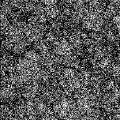
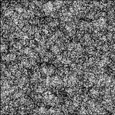
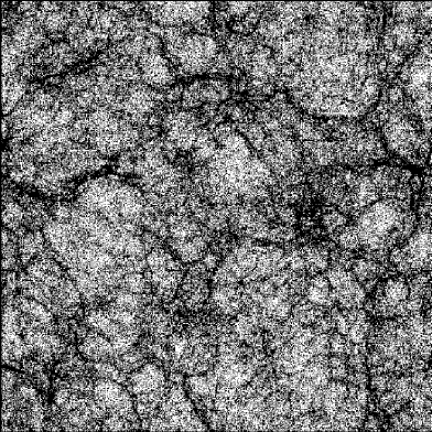
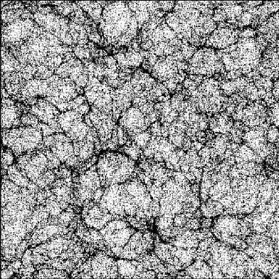
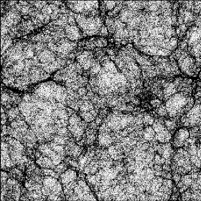
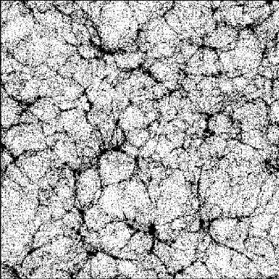
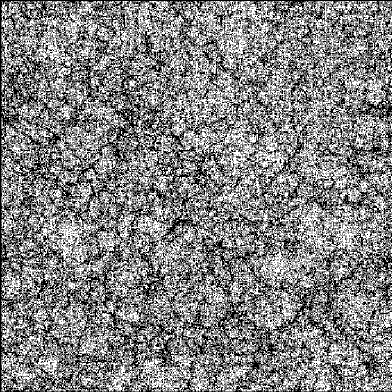
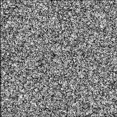
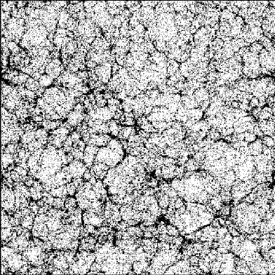
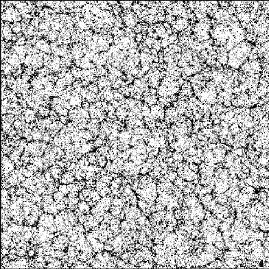
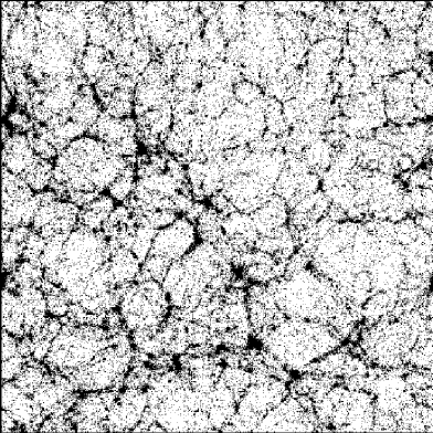
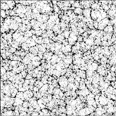
Figs 1 and 2 provide a visual account of the growth of structure in the four models. We show three epochs from the four different models: the initial conditions; an intermediate epoch; the final output epoch. The $n=-2$ simulations display a number of large-scale fluctuations which collapse to form large filaments and groups, whereas the $n=0$ simulations are characterized by a large number of tightly bound objects and a paucity of large-scale filamentary features, in accordance with the results of Efstathiou et al. [1988]. Fig. 1 also compares the glass start to the grid starts. In the glass start no features other than the prescribed fluctuations are observed, whereas the grid start shows faint lattice patterns which are still observable in the voids at the final epoch.

3.2 Power-law open and flat simulations

At late times the amplitude of the nonlinear power spectrum is very sensitive to the density of the universe, and strongly modulates the amplitude of the nonlinear clustering signal. This effect is important to quantify if one wishes to construct general models for evolving nonlinear power spectra. We investigated this density dependence by performing a further series of high resolution, $256^{3}$ particle, simulations for open universes where $\Omega=0.2$ at the final epoch and for flat universes where $\Omega=0.26$ and $\Lambda=0.74$ at the final epoch. The values for the density parameter were selected so that each full integration would span a large dynamic range in $\Omega$. The amplitude of the final box-scale mode was set slightly lower than in the $\Omega=1$ simulations, because of the greater small-scale nonlinearities that are generated in low-density models. For all of these simulations we have used the glass initial particle load. Table 2 displays all of the relevant simulation parameters.

3.3 The challenge of $n\rightarrow-3$

On small scales, the slope of the CDM power spectrum approaches $n\simeq-3$, so it is important to understand how such spectra evolve in the nonlinear regime. However, highly negative spectral indices have proven difficult to simulate (Efstathiou et al. 1988; Jain, Mo & White 1995; PD96; Jain & Bertschinger 1998), and this can be attributed to two main effects.

First, the number of particles must be high enough to simulate virialized clusters convincingly. Second, the finite size of the simulation volume means that the longest wavelength fluctuations that are present are $\lambda_{\kern 0.35002pt{\rm b}}=L\ ;\ k_{\kern 0.35002pt{\rm b}}=2\pi/L$. The absence of modes beyond the box scale induces an error in the nonlinear spectrum, since nonlinearity couples Fourier modes together and power leaks from large to small scales; the importance of this effect increases for increasingly negative spectral indices and dominates as $n$ approaches $-3$.

The error in the power spectrum due to these missing modes can be estimated from the linear power spectrum. We can quantify the missing variance as follows:

$$\sigma^{2}_{\rm miss}=\int^{\infty}_{0}\Delta_{\kern 0.35002pt{\scriptscriptstyle{\rm L}}}^{2}(k)\;\frac{dk}{k}-\sum\frac{1}{4\pi}{\Delta_{\kern 0.35002pt{\scriptscriptstyle{\rm L}}}^{2}(k^{\prime})\over(\ell^{2}+m^{2}+n^{2})^{3/2}}\ ,$$ (24)

where the sum is over all integer triples $(\ell,m,n)$ except $(0,0,0)$ and the wavenumber $k^{\prime}=k_{\kern 0.35002pt{\rm b}}(\ell^{2}+m^{2}+n^{2})^{1/2}$. Strictly speaking, both terms on the rhs are divergent for power-law spectra with $n\geq-3$. Nonetheless, if one imposes a sufficiently smooth cut-off at $k_{\rm cut}$ in the power spectrum, then the difference is well defined in the limit of $k_{\rm cut}\rightarrow\infty$.

We have estimated $\sigma^{2}_{\rm miss}$ numerically in this way for scale-free power spectra as a function of $n$. To about 1% accuracy the result is given by:

$$\sigma^{2}_{\rm miss}=\frac{\Delta_{\kern 0.35002pt{\scriptscriptstyle{\rm L}}}^{2}(k_{\kern 0.35002pt{\rm b}})}{3+n}F(3+n),$$ (25)

where $F(y)=1-0.31y+0.015y^{2}+0.00133y^{3}$ and this expression is valid for $-3\leq n\leq 1$. One can check the numerical result, not only by confirming it is insensitive to the precise value of $k_{\rm cut}$, but also for the special case $n=0$ where it is easy to see from geometric considerations that the value of $F(3)$ is $3/4\pi$. In the limit of $n\rightarrow-3$ the missing variance is well approximated by the quantity $\sigma^{2}_{\kern 0.35002pt{\rm err}}$ defined as:

$$\sigma^{2}_{\kern 0.35002pt{\rm err}}=\frac{\Delta_{\kern 0.35002pt{\scriptscriptstyle{\rm L}}}^{2}(k_{\kern 0.35002pt{\rm b}})}{3+n}\ .$$ (26)

So as to ensure that the missing variance does not become significant for our simulations, we have chosen to adopt the criterion

$$\sigma^{2}_{\kern 0.35002pt{\rm err}}\leq 0.04\ ,$$ (27)

for which the large-scale missing modes are safely linear.

It is for these reasons that the relatively low resolution (compared to modern standards) $32^{3}$ particle, $n=-2$ simulation of Efstathiou et al. [1988] could only reproduce the exact similarity solution for the power spectrum over a narrow range of expansion. Also, for the more recent high-resolution $256^{3}$ particle, $n=-2$ simulation of Jain & Bertschinger [1998], the box-scale power for their last three outputs violates the condition (27), rising to $\sigma^{2}_{\kern 0.35002pt{\rm err}}\simeq 0.4$ for the last epoch.

3.4 Simulation error and Layzer–Irvine energy

A test for the global accuracy of the integration of the equations of motion is to measure how well the Layzer–Irvine energy equation [1980, equation 24.7] is obeyed [1985]. One way to characterize this is through the change in the Layzer–Irvine integral, $I$, divided by the total potential energy $W$ (Couchman et al 1995):

$$I=K+W+\int\left[2K+W\right]\frac{da}{a}\ ,$$ (28)

where $K$ is the total kinetic energy. In Tables 1 and 2 we present the percentage error in each of the simulations. The accuracy of the integration decreases as the spectral index steepens and as $\Omega$ decreases, the least accurate integration being that of the open $n=0$ simulation, for which the global error at the final epoch was of the order 1.8%.

4 Measuring the power spectrum

The Fourier modes of the particle distribution can be determined exactly using the expression [1980]

$$\delta_{\bf k}=\frac{1}{N}\sum_{i=1}^{N}e^{i{\bf k}\cdot{\bf x}_{i}}\ .$$ (29)

Owing to the periodic boundary conditions, wavenumbers are restricted to be integer multiples of the fundamental mode, with an upper limit imposed by the finite sampling of the mesh: the Nyquist frequency,

$$k_{\kern 0.35002pt{\rm Ny}}=\frac{\pi}{\Delta x}\ ,$$ (30)

where $\Delta x=L/N_{\rm m}$ is the mesh spacing and $N_{\rm m}$ is the dimension of the mesh. The power spectrum can then be estimated through averaging over all of the modes in a thin shell in $k$ space:

$$\hat{P}(k)\equiv\left<\left|\delta_{k}\right|^{2}\right>=\frac{1}{m}\sum_{i=1}^{m}\left|\delta_{k_{i}}\right|^{2}.$$ (31)

where $m$ is the number of modes to be averaged. This method is computationally inefficient, with the required cpu time scaling as $MN$ for $M$ modes. A faster method is to distribute particles onto a cubical mesh and perform a Fast Fourier Transform (FFT). However, the assignment of mass to grid cells introduces some systematic effects which must be corrected; these issues will be discussed in detail in Section 4.2.

In the case of a 3D particle distribution, the task soon becomes memory limited, a $512^{3}$ FFT requiring roughly 0.5 Gbyte for a ‘real-real’ transform and 1 Gbyte for a ‘complex-complex’ transform. A solution to this problem was proposed by J98; we now detail this method, since it is critical for the present paper.

4.1 Chaining the power

Consider a 1D discrete density field $\delta(x)$, which is periodic over a length scale $L$ and which has a discrete Fourier transform given by equation (29). If we partition the density field using a coarse mesh with $M$ grid cells, then the density at the point $x$ can be described by the relation

$$\delta(x)=\delta\left(x^{\prime}+jL/M\right)\ ,$$ (32)

where $x^{\prime}$ is the position of the particle in its grid cell and $j$ labels the cell. If we now map all of the grid cells into one cell, then the reduced density field, which is now periodic on the scale $L/M$, is

$$\delta^{r}(x^{\prime})=\sum_{j=0}^{M-1}\delta(x^{\prime}+jL/M)\ .$$ (33)

The discrete Fourier transform of this reduced density field is then,

$$\delta_{k}^{r}=\frac{1}{N}\sum_{i=1}^{N}\exp(ikx_{i}^{\prime})=\frac{1}{N}\sum_{i=1}^{N}\exp[ik(x_{i}-jL/M)]\ .$$ (34)

Provided that the $k$-modes are integer multiples of the new fundamental mode, $k=\ell 2\pi/(L/M)$, then the last term in the exponential is a multiple of $2\pi$, so the modes of the reduced field are equivalent to the modes of the true field. There is, however, a reduction in the number of available modes, since the smaller volume of the coarse mesh gives a lower density of states.

4.2 Numerical effects on the power

There are three important numerical effects which can modify the ‘observed’ power spectrum from the true nonlinear signal: discreteness effects, charge assignment and force softening.

4.2.1 Discreteness effects

For a random distribution of particles with no imposed clustering, the power does not vanish. This result can be deduced by splitting 3D space into a large number of cubical cells, so that the occupation number of each cell is either $n_{i}=0$ or 1 (Peebles 1980). On computing the expectation of the power spectrum, we obtain the shot-noise spectrum

$$\left<\left|\delta_{k}\right|^{2}\right>=\frac{1}{N}\$$ (35)

which in dimensionless form is written

$$\Delta^{2}_{\kern 0.35002pt{\rm shot}}=\frac{4\pi}{N}\left[\frac{k}{k_{\kern 0.35002pt{\rm b}}}\right]^{3}.$$ (36)

This leads us to write the true power spectrum, in the limit of large $N$ [1991]

$$\Delta^{2}_{\rm true}(k)=\Delta^{2}_{\rm obs}(k)-\Delta^{2}_{\rm shot},$$ (37)

where $\Delta^{2}_{\rm obs}$ is the observed power from equation (31).

However, this correction is invalid for the glass and grid starts discussed in section 3. To determine the appropriate correction for these schemes we directly computed the power spectrum of the initial conditions and then used these empirical spectra to construct a simple correction model. In Fig. 3 (bottom) we show the raw power spectrum of the glass particle load for the initial conditions and two subsequent epochs from the $n=-2$ simulation. The glass power spectrum is characterized by a two-power-law spectrum: on intermediate scales the spectrum is steep, roughly the $n=4$ ‘minimal slope’ (see section 28 of Peebles 1980) and at smaller scales this breaks to a shot noise spectrum. Furthermore, the bottom panel of Fig. 3 shows that the discreteness spectrum does not appear to evolve; we can therefore use the initial conditions to determine a discreteness correction that can be applied to correct the observed power at all subsequent epochs. This correction can be modelled as a transition between shot noise on small scales and the almost minimal spectrum on intermediate scales:

$$\Delta^{2}_{\kern 0.35002pt{\rm glass}}=\left[\left(\Delta^{2}_{\kern 0.35002pt{\rm shot}}\right)^{-1/\alpha}+\left(\Delta^{2}_{\min}\right)^{-1/\alpha}\right]^{-\alpha}\ ,$$ (38)

where $\alpha=0.3$ and $\Delta_{\min}^{2}=(A\,k/k_{\kern 0.35002pt{\rm b}})^{\beta}$, with best fitting values $A=0.0062$ and $\beta=6.8$.

Figure 3: (Top) The glass-discreteness corrected (squares) and uncorrected power spectrum (stars) of the glass $n=-2$ simulation at an epoch $a=0.55$. We show the linear fluctuation spectrum (dashed line), which demonstrates that the box scale mode is still linear, the nonlinear spectrum according to the scaling formula of PD96 (thin solid line), a shot noise spectrum (dot-dashed line) and our two power-law discreteness model outlined in the text (thick solid line). (Bottom) Three epochs from the early stages of the same $n=-2$ simulation. From bottom to top epochs are $a=0.025$ (squares), 0.1 (circles) and 0.3 (stars). This demonstrates that the discreteness spectrum does not evolve and also that the linear spectrum has been correctly established early on. Again, the lines are as in the top panel, with the thick solid line representing our fit to the discreteness spectrum.

For the grid, or ‘quiet’ start, the issue of a discreteness correction is fairly subtle, since there is initially no power added to the distribution by particle placement except on the scales of the Nyquist frequency of the mesh. However, as the simulation evolves under gravity, the sparseness of particles on small scales forms a power spectrum similar to a shot noise term on those scales. At late times this can be remedied by subtracting the Poisson spectrum from the raw power, since the large- and intermediate-scale modes in the evolved distribution are of higher amplitude than the shot-noise spectrum. At early times, when the true power is of relatively low amplitude, this approach is incorrect. We avoid the problem by excluding points whose amplitudes are below the Poisson spectrum on the equivalent scale.

Fig. 4 (top) compares the uncorrected power spectra for the glass and grid starts measured from the $n=-2$ simulations at two epochs $a=0.4$ and $a=0.55$. We observe that the nonlinear loci defined by the data for these two simulations are consistent and show no memory of the initial particle load. The only noticeable discrepancy between the two simulations is the difference in large-scale power; this arises because the simulations are independent realizations. Fig. 4 (bottom) contrasts the discreteness-corrected spectra; this shows that consistent final results are obtained through simulating with grid or glass initial conditions.

Figure 4: (Top) Comparison of discreteness uncorrected power spectra measured from the quiet start (squares) and glass start (stars) $n=-2$ simulations at epochs $a=0.4$ and 0.55. Line styles are as in Fig. 3. (Bottom) Comparison of discreteness corrected power spectra for the same outputs from the two simulations.

4.2.2 Mass assignment

The assignment of mass onto the FFT mesh produces a finite sampling error of the true density field. This problem was investigated for power spectra by Baugh & Efstathiou [1994], who proposed that equation (37) for the true field should be modified to

$$\Delta^{2}_{\kern 0.35002pt{\rm true}}(k)=\frac{\Delta^{2}_{\kern 0.35002pt{\rm obs}}(k)-\Delta^{2}_{\kern 0.35002pt{\rm disc}}(k)}{w(y)}\ ;\ \ \ \ y=k/k_{\rm m}\ ,$$ (39)

where $w(y)$ is the Fourier transform of the mass assignment window function, $\Delta^{2}_{\kern 0.35002pt{\rm disc}}(k)$ is the appropriate discreteness correction and $k_{\rm m}=2\pi/\Delta x$ is the wave number associated with the inter-mesh spacing $\Delta x$. However, we believe that there is a small flaw in their method. Any discreteness correction should be made subsequent to the correction due to mass assignment, since the discreteness correction accounts for the representation of a continuous field with a point-like distribution. We therefore implement the correction as

$$\Delta^{2}_{\kern 0.35002pt{\rm true}}(k)=\frac{\Delta^{2}_{\kern 0.35002pt{\rm obs}}(k)}{w(y)}-\Delta^{2}_{\kern 0.35002pt{\rm disc}}(k)\ ;\ \ \ \ y=k/k_{\rm m},\ .$$ (40)

Several schemes exist for transferring mass onto the Fourier mesh. The simplest scheme is nearest grid point (NGP), which assigns all of the mass to the closest mesh point. More sophisticated methods such as cloud-in-cell (CIC) and triangular-shaped-cloud (TSC) attempt to smear the mass across a number of mesh points. We have adopted the TSC scheme to assign particles to the mesh. However, the detailed correction is unimportant when using the chained-power method of J98. Results at high $k$ can be obtained either by making substantial binning corrections to the main FFT mesh, or by moving to a sub-mesh of higher resolution. In practice, we make this transition before the corrections from binning become significant. Finally, Baugh & Efstathiou showed that, even after correcting for the window function, the power is affected by aliasing close to the Nyquist frequency. Again, when following the method described in Section 4.1, aliasing errors can be avoided by only using modes that are a safe distance from the Nyquist frequency of a given (sub)mesh (a factor of 2, in practice).

4.2.3 Force softening

The softening of the Newtonian force in the PP part of the $N$-body calculation (described in Section 3) induces an error in the integration of particle trajectories for close pairs. By considering the fractional error in the softened force from the true Newtonian force, we can impose some constraints on the small-scale cutoff, below which numerical effects dominate the clustering in our simulations. For our spline-kernel force softening, we expect numerical effects to suppress the true power on scales of a few times the softening length. This corresponds to $k/k_{\rm b}\sim 1700$.

The simplest way to discriminate between the true nonlinear solution and numerical artefacts is to use the self-similar evolution of the scale-free simulations. Since the numerical features are of fixed comoving length, the true density field will scale under the transformations that were described in Section (2.4), whereas the numerical effects do not. We provide evidence for this in section 5.

5 Numerical results

5.1 Similarity solution

Figure 5: Nonlinear power plotted against linear power (points) for the four scale-free simulations. For clarity, the data have been separated from each other by one order of magnitude in the $y$-direction, with the $n=0$ data untranslated. To determine the linear power given a nonlinear data point, the appropriate linear scale is required. In the HKLM method, this is found using the transformation $k_{\kern 0.31502pt{\scriptscriptstyle{\rm L}}}=[1+\Delta^{2}_{\kern 0.31502pt{\scriptscriptstyle{\rm NL}}}(k_{\kern 0.31502pt{\scriptscriptstyle{\rm NL}}})]^{-1/3}k_{\kern 0.31502pt{\scriptscriptstyle{\rm NL}}}$. The solid line represents the fitting formula for the Einstein–de Sitter models presented in Appendix B; the dashed line represents the PD96 fitting formula; the dotted lines are the fits using the formula of JMW95.

Figure 6: Nonlinear slope of the power spectrum versus spectral index. Points are measured from the scale-free simulation power spectra. The solid line represents the stable-clustering prediction. The dot-dash lines correspond to the predictions of the halo model (Ma & Fry 2000b), with an assumed $\epsilon=0.4$ and $0.0\leq\beta_{0}\leq 1.0$. The dotted lines correspond to the halo model prediction with $\beta_{0}=0.25$ and $0.4\leq\epsilon\leq 1.0$.

Fig. 5 shows the data for the four scale-free models in the HKLM form: nonlinear power on the nonlinear scale plotted as a function of the linear power on the linear scale. For clarity, the data have been separated from each other by one order of magnitude in the $y$-direction, with the $n=0$ data untranslated. In order to determine the linear scale and power that correspond to a given nonlinear data point, we use the nonlinear scaling relation (13). Explicitly, given a nonlinear data point $k_{i\kern 0.35002pt{\scriptscriptstyle{\rm NL}}},\Delta^{2}_{i\kern 0.35002pt{\scriptscriptstyle{\rm NL}}}$, its linear counterpart is

$$k_{i\kern 0.35002pt{\scriptscriptstyle{\rm L}}}=(1+\Delta^{2}_{i\kern 0.35002pt{\scriptscriptstyle{\rm NL}}})^{-1/3}k_{i\kern 0.35002pt{\scriptscriptstyle{\rm NL}}}\ ;\hskip 28.45274pt\Delta^{2}_{i\kern 0.35002pt{\scriptscriptstyle{\rm L}}}=\left(\frac{k_{i\kern 0.35002pt{\scriptscriptstyle{\rm L}}}}{k_{0}}\right)^{3+n},$$ (41)

where $k_{0}$ is a time-dependent normalization wavenumber defined by $\Delta^{2}(k_{0})\equiv 1$ and we have assumed an initial power-law power spectrum for this example.

When plotted in this form the scaling nature of these models is apparent. The power spectra measured from multiple epochs of the simulations precisely overlay to define a single locus for each of the spectral models considered. We confirm the observation of JMW95 and PD96 that different spectral models produce different amounts of nonlinear growth and that the more negative the spectral index the steeper the locus in this plane. Fig. 5 also shows that the $n=-2$ simulations have produced a single, tightly defined locus. This was not observed in previous studies (see Fig. 1 of Jain 1997, Fig. 1 of PD96 and Fig. 7 of Jain & Bertschinger 1998). This failure of scaling in earlier $n=-2$ results was probably attributable to saturation of the box-scale mode.

The evolution in the data can be roughly broken down into three regimes, the linear, the quasi-linear and the nonlinear. General observations made about these regimes are:

1. Linear: $\Delta_{\kern 0.35002pt{\scriptscriptstyle{\rm NL}}}^{2}<1$: the ‘nonlinear’ power for all of the models converges to the linear power.

2. Quasi-linear: $2<\Delta_{\kern 0.35002pt{\scriptscriptstyle{\rm Q}}}^{2}<30$: the slope of the $f_{\kern 0.35002pt{\scriptscriptstyle{\rm NL}}}$ curves are steep. Modelling the data in this regime with a single power-law of the form, $\Delta_{\kern 0.35002pt{\scriptscriptstyle{\rm Q}}}^{2}\propto\left[\Delta_{\kern 0.35002pt{\scriptscriptstyle{\rm L}}}^{2}\right]^{\alpha}$, we find for $n=-2$, $-1.5$, $-1$ and 0, that the spectral slopes are $\alpha=3.62\pm 0.03$, $3.38\pm 0.05$, $3.12\pm 0.06$ and $2.96\pm 0.1$. This is reasonably close to the suggestion of Padmanabhan [1996] that $\smash{\Delta^{2}_{\kern 0.35002pt{\scriptscriptstyle{\rm Q}}}\propto[\Delta^{2}_{\kern 0.35002pt{\scriptscriptstyle{\rm L}}}]^{3}}$, although there is a clear trend with $n$ that is not expected in Padmanabhan’s argument. This departure from a simple scaling relation is also supported by the results from loop-correction perturbation theory (see Fig. 19 of Scoccimarro & Frieman 1996). However, it may be argued that extended perturbation theory will fail at such large nonlinearities. One caveat is that it has been suggested that the nonlinear scaling relation may only truly be valid for $\bar{\xi}$ [2001] and not $\Delta^{2}$. The small scatter observed in Fig. 5 leads us to believe that this might not be the case.

3. Nonlinear: $\Delta^{2}_{\kern 0.35002pt{\scriptscriptstyle{\rm NL}}}>30$: the $f_{\kern 0.35002pt{\scriptscriptstyle{\rm NL}}}$ curves break away from the steep evolution which characterized the quasi-linear growth to form loci that are much shallower. Again, we have performed a simple power-law fit to the data of each locus. We find that for $\Delta^{2}_{\kern 0.35002pt{\scriptscriptstyle{\rm NL}}}>50$ the $n=-2$ data have a nonlinear slope $\alpha=1.05\pm 0.09$, and for $\Delta^{2}_{\kern 0.35002pt{\scriptscriptstyle{\rm NL}}}>100$ the $n=-1.5$, $-1$ and 0 data have nonlinear asymptotes of $\alpha=0.87\pm 0.04$, $\alpha=1.08\pm 0.04$ and $\alpha=0.99\pm 0.04$. This result is interesting for two reasons. Firstly, within the scatter in the simulations there appears to be little dependence on the initial spectrum for the nonlinear slope. Secondly, it is in clear contradiction to stable clustering, which predicts that $\alpha=3/2$. We note that this result agrees with the findings of Bagla, Engineer & Padmanabhan [1998] for clustering in 2D. However, Fukushige & Suto [2001] found that the stability on small scales, as measured from peculiar velocities, was not preserved locally but did apply globally. Our results do not agree with this.

The shallow slope at high $k$ may be interpreted in terms of the halo model. Ma & Fry (2000b) derived the following asymptotic limit for the power spectrum:

$$\Delta^{2}(k)\propto k^{\gamma};\hskip 14.22636pt\gamma=\frac{18\beta-\epsilon(n+3)}{2(3\beta+1)},$$ (42)

where $\beta\simeq 0.8\beta_{0}$ is the power-law that governs the mass dependence of halo concentrations: $c=r_{v}/r_{s}=(M/M_{*})^{\beta_{0}}$; $r_{v}$ and $r_{s}$ being the virial and characteristic radius; and $\epsilon$ is the power-law index that governs the low-mass tail of the mass function: $dn/dM\propto\nu^{\epsilon};\nu\propto 1/\sigma(M)$. Realistic values for $\epsilon$ and $\beta_{0}$ are $0.4\leq\alpha\leq 1.0$ and $0.0\leq\beta_{0}\leq 0.5$. This is illustrated in Fig. 6, which shows the nonlinear power spectral index $\gamma$ as a function of the initial spectral index $n$. The values of $\gamma$ were obtained from the above nonlinear scaling relations, $\Delta^{2}_{\kern 0.35002pt{\scriptscriptstyle{\rm NL}}}\propto[\Delta^{2}_{\kern 0.35002pt{\scriptscriptstyle{\rm L}}}]^{\alpha}$, using the relationship (PD96)

$$\Delta^{2}_{\kern 0.35002pt{\scriptscriptstyle{\rm NL}}}\propto k_{\kern 0.35002pt{\scriptscriptstyle{\rm NL}}}^{\gamma};\hskip 14.22636pt\gamma=\frac{3\alpha(n+3)}{3+\alpha(n+3)}\ .$$ (43)

We find $\gamma=0.77,\;0.91,\;1.26,\;1.49$ for spectral indices $n=-2,\;-1.5,\;-1.0,\;0.0$. Comparing these measured values against the two predictions from equation (7) and (42), we see that $\gamma$ increases with the steepness of the spectrum, but that the data fall below the stable clustering prediction. In terms of the halo model, if one assumes $\epsilon=0.4$ in accord with Sheth & Tormen (1999), then a strong dependence of $\beta_{0}$ on $n$ is required in order to match the measured data. On the other hand, if one adopts a value $\beta_{0}=0.25$ in the middle of the current measured values, then it is impossible to match the measured data with any value of $\epsilon$ in the plausible range 0.4 to 1.0. In summary, equation (42) seems unable to predict the observed trend of $\gamma(n)$ in a natural manner. This is puzzling, since we will show below that the general ideas of the halo model work very well in describing our data. One possibility is that equation (42) is valid only on scales smaller than those probed by current simulations.

Also, in Fig. 5 we contrast our data with the fitting formula of JMW95 and PD96 (see Appendix A.1 and A.2 for these formulae). Both models work reasonably well in the quasi-linear regime, but with significant discrepancies. The $n=-2$ results are poorly fit by both models, with the power being in general underestimated; PD96 gives the poorer fit, and underestimates the power by up to a factor 2. The $n=-1.5$ locus is fairly well characterized by the JMW function, but underestimated by PD96. The $n=-1$ results are fairly well fit by both models, except around the break between linear and quasi-linear slopes, where the functions overestimate the power. Finally, the $n=0$ locus is slightly overestimated at the linear to quasi-linear break by PD96 and underestimated by JMW95. We have produced a new HKLM fitting formula that accurately fits the individual Einstein–de Sitter models, the results of which are shown in Fig. 5 as the thin solid line. The formula is described in Appendix B.

Figure 7: (Top) HKLM plot for the open models. (Bottom) HKLM plot for the flat low-density models with a cosmological constant. Again, for clarity, the data have been separated from each other by one order of magnitude in the $y$-direction, with the $n=0$ data untranslated. For each model five epochs are shown, these are: $a=0.6,0.7,0.8,0.9,1.0$, with the lowest locus for each model corresponding to the $a=0.6$ epoch. In terms of the mass density parameter of the universe, these epochs correspond to: $\Omega=0.294,0.263,0.238,0.217,0.200$ for the open models and $\Omega=0.619,0.505,0.407,0.325,0.260$ for the $\Lambda$ models. As in Fig. 5 the solid lines represent the fitting formula for the Einstein–de Sitter models presented in Appendix B; the dashed lines represent fits from the PD96 function.

5.2 Low-density power-law models

In Fig. 7 we show how the nonlinear behaviour of the power-law models deviates from the scale-free solutions (solid lines) as the background density is lowered. Again, for clarity, the data have been separated from each other by one order of magnitude in the $y$-direction, with the $n=0$ data untranslated. In the linear regime, we again find that the nonlinear data follow the linear power. In the quasi-linear regime, $2<\Delta_{\kern 0.35002pt{\scriptscriptstyle{\rm NL}}}^{2}<80$, as $\Omega$ decreases, the locus defined by the data increases in amplitude relative to the scale-free models and the power-law slope steepens. This density-dependent evolution of $f_{\kern 0.35002pt{\scriptscriptstyle{\rm NL}}}$ in the quasi-linear regime was not apparent in previous studies (see PD96). The quasi-linear slope steepens as both $n$ and $\Omega$ decrease. In the nonlinear regime, $\Delta^{2}_{\kern 0.35002pt{\scriptscriptstyle{\rm NL}}}>80$, we again observe that the slope of $f_{\kern 0.35002pt{\scriptscriptstyle{\rm NL}}}$ is lower than the $3/2$ value that is required by stable clustering.

In Fig. 7, we also compare the data with the density dependent fitting formula of PD96. Again, the formula underestimates the shallow spectra and slightly overestimates the steeper spectra. However, the more striking discrepancy is that the formula suppresses the onset of density dependent growth until evolution is far into the nonlinear regime, and then tends to overestimate the highly nonlinear power. These discrepancies can in fact be seen in the comparison with the simulation data used by PD96. However, this library of small ($N=80^{3}$) simulations was in most cases unable to probe beyond $\Delta^{2}_{\kern 0.35002pt{\scriptscriptstyle{\rm NL}}}\simeq 200$, and so the deviations never became substantial.

The failure of the JMW95 and PD96 functions to accurately model the Einstein–de Sitter data and account for the density dependence of nonlinear growth has clearly been shown. On attempting to fit this data set using the standard HKLM-PD96 procedure we were able to produce an improved formula with an rms precision of 12%. However, on attempting to integrate the CDM models into the formulation, we could not find a satisfactory way to assign an effective spectral index to the models. We therefore decided to pursue an alternative approach to the problem of general nonlinear fitting functions, which proved to be more accurate.

Figure 8: Comparison of the full halo-model calculation as described in the text (thick solid lines) with the CDM data (points). Also shown is the halo-model fitting formula from this work (thin solid lines). For clarity the four CDM models have been separated from each other by one order of magnitude in the y-direction, with the $\tau$CDM data untranslated.

6 The halo model fitting function

In this Section, we attempt to describe the above nonlinear results by means of concepts abstracted from the ‘halo model’ [2000, 2000, 2000a]. The basic approach suggested by the halo model is to decompose the density field into a distribution of isolated haloes. Correlations in the field then arise on large scales through the clustering of haloes with respect to each other and on small scales through the clustering of dark matter particles within the same halo. This then leads to a total nonlinear power spectrum

$$P_{\kern 0.35002pt{\scriptscriptstyle{\rm NL}}}(k)=P_{\kern 0.35002pt{\scriptscriptstyle{\rm Q}}}(k)+P_{\kern 0.35002pt{\scriptscriptstyle{\rm H}}}(k),$$ (44)

where $P_{\kern 0.35002pt{\scriptscriptstyle{\rm Q}}}(k)$ is the quasi-linear term that represents the power generated by the large-scale placement of haloes and where $P_{\kern 0.35002pt{\scriptscriptstyle{\rm H}}}(k)$ describes the power that results from the self-correlation of haloes.

It is remarkable that such a simple decomposition appears to work well in describing the main characteristics of the two-point correlations of the cosmological mass density. It is maybe yet still more impressive when one considers that the present formulation knows nothing of the large-scale filamentary structure of the density field (which is governed by the correlation function of halo centres). Indeed this deficiency was recently pointed out and addressed by Scoccimarro & Sheth [2002]

In Fig. 8 we directly compare the halo-model calculations (thick solid lines) with the CDM simulations of J98 (data points – see section 6.4 for full description). Also shown is the halo-model fitting function that we present later (thin solid lines – see Appendix C). The halo model calculations are exactly those of Peacock & Smith (2000). From the figure, it can clearly be seen that the calculations qualitatively reproduce the data for all of the models, but that in detail only match SCDM and $\tau$CDM closely. Furthermore when one attempts to model the power-law spectra the results are worse, with the $n=0$ case being an extreme example (see the later discussion). Thus our aim in what follows will therefore be to produce a simple fitting formula that draws on the broad elements of the halo model, such as the above decomposition of the power spectrum into two linearly summed terms, but which is of very high accuracy.

6.1 The quasi-linear term

Consider the quasi-linear part first. Seljak [2000], Ma & Fry [2000a] and Scoccimarro et al. [2001] assumed that one should use linear theory filtered by the effective window corresponding to the distribution of halo masses, convolved with their density profiles and a prescription for their bias with respect to the underlying mass field:

$$P_{\kern 0.35002pt{\scriptscriptstyle{\rm Q}}}(k)=P_{\kern 0.35002pt{\scriptscriptstyle{\rm L}}}(k)\left[\frac{1}{\bar{\rho}}\int dM\;b(M)\,n(M)\;\tilde{\rho}(k,M)\right]^{2},$$ (45)

where $n\left(M\right)dM$ is the mass function, $\tilde{\rho}\left(k,M\right)$ is the Fourier transform of the density profile and $b(M)$ is the bias field of dark matter halo seeds. Peacock & Smith [2000] made the simpler assumption that the quasilinear term corresponded to pure linear theory:

$$P_{\kern 0.35002pt{\scriptscriptstyle{\rm Q}}}(k)=P_{\kern 0.35002pt{\scriptscriptstyle{\rm L}}}(k).$$ (46)

This is equivalent to equation (45) on large scales, since in this limit the filtering effect of haloes is negligible, and we must have

$$\frac{1}{\bar{\rho}}\int dM\;b(M)\,M\,n(M)=1\ .$$ (47)

Neither of these approaches is really satisfactory, since $P_{\kern 0.35002pt{\scriptscriptstyle{\rm H}}}$ comes to dominate only at scales where linear theory must break down to some extent ($\Delta^{2}_{\rm L}\sim 1$). Quasi-linear effects must modify the relative correlations of haloes away from linear theory, irrespective of whatever allowance may be made for the finite sizes of haloes. One way of seeing this is via the scaling part of the HKLM procedure: see equations (13). This shift of scales from gravitational collapse causes a significant change in power at wavenumbers where $\Delta^{2}_{\kern 0.35002pt{\scriptscriptstyle{\rm L}}}$ is of order unity – which is just the point where the filtering effects of the largest haloes will also start to be important. An alternative point of view is provided by perturbation theory, which suggests that quasilinear effects should tend to suppress power for $n>-1.4$, but enhance power for more negative indices (e.g. section 4.2.2 of Bernardeau et al. 2001). Again, such effects cannot be cleanly separated from the convolving effects of halo profiles. We therefore take an empirical approach, allowing the quasilinear effects to depend on $n$. Since the philosophy of the halo model is that $\Delta^{2}_{\kern 0.35002pt{\scriptscriptstyle{\rm Q}}}$ should be negligible on small scales, we also build in a truncation at high $k$:

$$\Delta^{2}_{\kern 0.35002pt{\scriptscriptstyle{\rm Q}}}(k)=\Delta^{2}_{\kern 0.35002pt{\scriptscriptstyle{\rm L}}}(k){\left[1+\Delta^{2}_{\kern 0.35002pt{\scriptscriptstyle{\rm L}}}(k)\right]^{\beta_{n}}\over 1+\alpha_{n}\Delta^{2}_{\kern 0.35002pt{\scriptscriptstyle{\rm L}}}(k)}\exp{-f(y)};\ \ \ y\equiv k/k_{\sigma}.$$ (48)

where $k_{\sigma}$ is a nonlinear wavenumber, defined below in Section 6.3 $\alpha_{n}$ and $\beta_{n}$ are spectral dependent coefficients and $f(y)$ is the polynomial $y/4+y^{2}/8$ that governs the decay rate. We adopt this expression for all spectra.

6.2 The halo term

In the halo model the self-halo term is [2000, 2000, 2000a, 2001]

$$P_{\kern 0.35002pt{\scriptscriptstyle{\rm H}}}(k)=\frac{1}{\bar{\rho}^{2}\left(2\pi\right)^{3}}\int dM\;n(M)\left|\tilde{\rho}\left(k,M\right)\right|^{2}.$$ (49)

In order to model this we want something that looks like a shot-noise spectrum on large scales, but is progressively reduced on small scales by the filtering effects of halo profiles and the mass function. In terms of the dimensionless power spectrum, a candidate form for this is

$$\Delta^{2\ \prime}_{\kern 0.35002pt{\scriptscriptstyle{\rm H}}}(k)={a_{n}\;y^{3}\over 1+b_{n}\;y+c_{n}\;y^{3-\gamma_{n}}};\quad\quad y\equiv k/k_{\sigma}\ ,$$ (50)

where $(a_{n},b_{n},c_{n},\gamma_{n})$ are dimensionless numbers that depend on the spectrum. However, with $P_{\kern 0.35002pt{\scriptscriptstyle{\rm H}}}$ defined in this way, the formalism defined by equation (44) breaks down for steep spectra. The self-halo power clearly dominates at small $k$ for any spectrum that is asymptotically $n>0$ (e.g. all CDM models). This has been independently noted by Sheth & Cooray (2001). The halo model thus fails to respect low-order perturbation theory in such cases, and this is a clear defect of the model.

In order to solve this problem, the self-halo power must become steeper than Poisson on the largest scales. This makes sense if we think of the halo model as a two-stage process: (i) fragment a uniform mass distribution into a set of haloes; (ii) move these haloes according to a superimposed large-scale displacement field. Since the first stage conserves mass, the large-scale power spectrum must approach a ‘minimal’ form with $n=2$ (e.g. section 28 of Peebles 1980). If one conserves momentum also, the minimal spectrum becomes even steeper: $n=4$. It is a moot point which of these is the appropriate asymptote for this problem, since the two-stage view of the halo model is only a heuristic argument. Since we will never wish to consider spectra that are asymptotically much steeper than $n=1$, it will suffice to force the $n=0$ self-halo term to approach $n=2$ on sufficiently large scales. This can be achieved if equation (50) is modified as follows

$$\Delta^{2}_{\kern 0.35002pt{\scriptscriptstyle{\rm H}}}(k)={\Delta^{2\ \prime}_{\kern 0.35002pt{\scriptscriptstyle{\rm H}}}(k)\over 1+\mu_{n}y^{-1}+\nu_{n}y^{-2}};\ \ \ y\equiv k/k_{\sigma}$$ (51)

where we have introduced a term in $k^{4}$ in order to soften the transition to the $k^{5}$ slope. Again, the parameters $\mu_{n}$ and $\nu_{n}$ are spectral dependent coefficients.

6.3 The nonlinear scale

In order to implement these arguments, we need an appropriate general definition of the nonlinear scale (see Section 2.4), which should be related to the characteristic mass in the halo mass function. As studies over many years have shown with increasing accuracy [1974, 1999, 2001], the halo mass function appears to depend only on the dimensionless fluctuation amplitude

$$\nu\equiv\delta_{c}/\sigma(R,t),$$ (52)

where $\delta_{c}$ is a constant of order unity, usually identified with the linear over-density for collapse in the spherical model and $R$ is the effective filter radius. The multiplicity function for haloes, which is defined as the fraction of mass carried by haloes with mass in a logarithmic interval, peaks for systems where $\sigma(R,t)$ is of order unity, and we can therefore choose to define the nonlinear scale in this way:

$$\sigma(k_{\sigma}^{-1},t)\equiv 1\ .$$ (53)

This definition of scale depends on the functional form chosen to filter the spectrum, but the main effects of changes in this choice can be absorbed into the fitting coefficients. We therefore take the convenient choice of a Gaussian filter:

$$\sigma^{2}(R_{\rm G},t)\equiv\int\Delta^{2}_{\kern 0.35002pt{\scriptscriptstyle{\rm L}}}(k,t)\,\exp(-k^{2}R_{\rm G}^{2})\;d\ln k.$$ (54)

With this choice of filter, scale-free spectra have

 

$${\Delta_{\rm L}^{2}(k,t)}$$

  (55)

6.4 Application to CDM

Figure 9: Variation of effective spectral index (top panel) and curvature (bottom panel) as a function of the rms fluctuation in Gaussian spheres of radius $R_{\rm G}$, for the four cosmological models considered. Note the lower $\sigma_{8}$ values that corresponded to the big-box simulations has been assumed for the SCDM and $\tau$CDM models.

Figure 10: Dependence of the nonlinear wave-number $k_{\sigma}$ (top panel), effective spectral index $n_{\rm eff}$ (middle panel) and curvature parameter $C$ (bottom panel) on the shape parameter $\Gamma$ and normalization $\sigma_{8}$ of the linear power spectrum. The parameters $n_{\rm eff}$ and $C$ are degenerate under $\Gamma$ and $\sigma_{8}$. This degeneracy is, however, broken by the nonlinear wavenumber.

Table 3: The cosmological parameters of the $N=256^{3}$ CDM simulations from J98. For these CDM models $\Gamma\equiv\Omega h$ is the shape parameter of the spectrum, $\sigma_{8}$ is the rms fluctuation in spheres of $8{\,h^{-1}\,\rm Mpc}$ and $h$ is the Hubble parameter

Model	$\Gamma$	$\sigma_{8}$	$\Omega$	$\Lambda$	$h$	$L/{\,h^{-1}\,\rm Mpc}$
SCDM	0.50	0.51	1.0	0.0	0.5	239.5
SCDM	0.50	0.6	1.0	0.0	0.5	84.55
$\tau$CDM	0.21	0.51	1.0	0.0	0.5	239.5
$\tau$CDM	0.21	0.6	1.0	0.0	0.5	84.55
$\Lambda$CDM	0.21	0.90	0.3	0.7	0.7	239.5
$\Lambda$CDM	0.21	0.90	0.3	0.7	0.7	141.3
OCDM	0.21	0.85	0.3	0.0	0.7	239.5
OCDM	0.21	0.85	0.3	0.0	0.7	141.3

We have generalized our formula to fit the Virgo and GIF CDM simulations from J98, which comprise four models: SCDM; $\tau$CDM; $\Lambda$CDM; OCDM. Table 3 lists the cosmological parameters for these models. The data are publicly available from http://www.mpa-garching.mpg.de/Virgo/. We have re-measured the power spectrum for the epochs $z=0.0,\;0.5\;1.0\;2.0$ and $3.0$ for both the Virgo and GIF data, the results are presented in Figs. 14 and 15. The transfer function for these simulations was that of Efstathiou, Bond & White [1992]:

$$\Delta^{2}(k)=\frac{Ak^{4}}{\left\{1+[aq+(bq)^{3/2}+(cq)^{2}]^{\nu}\right\}^{2/\nu}}$$ (56)

where $q=k/\Gamma$, $a=6.4\;{\,h^{-1}\,\rm Mpc}$, $b=3{\,h^{-1}\,\rm Mpc}$, $c=1.7{\,h^{-1}\,\rm Mpc}$. The normalization constant $A$ is chosen by fixing $\sigma_{8}$.

In order to model these more general curved spectra, we define an effective spectral index via

$$3+n_{\rm eff}\equiv-\left.{d\ln\sigma^{2}(R,t)\over d\ln R}\right|_{\sigma=1}\ .$$ (57)

Since the mass function should depend mainly on the Taylor expansion of $\sigma$ about the nonlinear scale, we also allow dependence on the spectral curvature:

$$C\equiv-\left.{d^{2}\ln\sigma^{2}(R,t)\over d\ln R^{2}}\right|_{\sigma=1}.$$ (58)

For the case of a Gaussian filter these expressions have the explicit forms,

$$3+n_{\rm eff}=\frac{2}{\sigma^{2}}\left.\int d\ln k\;\Delta^{2}_{\kern 0.35002pt{\scriptscriptstyle{\rm L}}}(k,t)\;y^{2}\exp{\left(-y^{2}\right)}\right|_{\sigma=1}$$ (59)

and

$$C = \left(3+n_{\rm eff}\right)^{2}+\frac{4}{\sigma(R)^{2}}\quad\times$$ (60)

$$\left.\int d\ln k\;\Delta^{2}_{\kern 0.35002pt{\scriptscriptstyle{\rm L}}}(k,t)\;\left(y^{2}-y^{4}\right)\exp{\left(-y^{2}\right)}\right|_{\sigma=1},$$

where $y=kR_{\rm G}$ and where the explicit time dependence of the power spectrum has been kept to indicate the redshift dependence of the effective quantities. In Table 4 we list the nonlinear wavenumber, effective spectral index and curvature of the spectrum on the nonlinear scale for the four Virgo (big-box) CDM models, generated according to the above prescription.

Table 4: The nonlinear wavenumber $k_{\sigma}$ in units of ${\,h\,\rm Mpc^{-1}}$, the effective spectral index $n_{\rm eff}$ and curvature $C$ of the spectrum on the nonlinear scale, for the four CDM models listed in the text.

Model	$k_{\sigma}$	$n_{\rm eff}$	$C$
SCDM	0.574	$-1.455$	0.411
$\tau$CDM	0.735	$-1.850$	0.305
$\Lambda$CDM	0.306	$-1.550$	0.384
OCDM	0.332	$-1.581$	0.375

Fig. 9 shows the variation of the effective spectral index (top panel) and curvature (bottom panel) for the four Virgo CDM models with the rms fluctuation measured in Gaussian spheres of effective radius $R_{\rm G}$. The effective spectral index is quite sensitive to whether it is defined at $\sigma=1$ or at some other value. However, including the curvature (which depends much more weakly on $\sigma$), means that this uncertainty is automatically allowed for. With the nonlinear scale and effective spectral index and curvature as defined through equations (53-58), we find that we can accurately model CDM spectra. As expected, Fig. 9 shows that the OCDM and $\Lambda$CDM models are almost indistinguishable: both possess nearly identical linear power spectra, with only a slight difference in normalization. The $\tau$CDM model has the shallowest effective spectral index, almost approaching $n=-2$ and the SCDM model has the steepest, with $n=-1.4$. The power-law models that we have simulated encompass this range of $n_{\rm eff}$. Thus, we are confident that the new fitting function will be constrained by the appropriate range of spectral models, with the notable exception of the $z>3$ $\tau$CDM data for which $n_{\rm eff}<-2$. These models are the sole basis for the fitting formulae in the $n<-2$ regime.

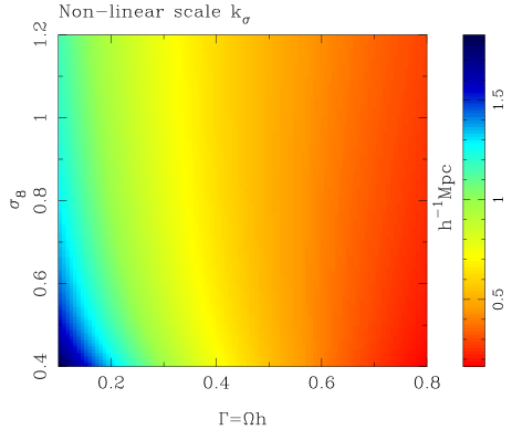
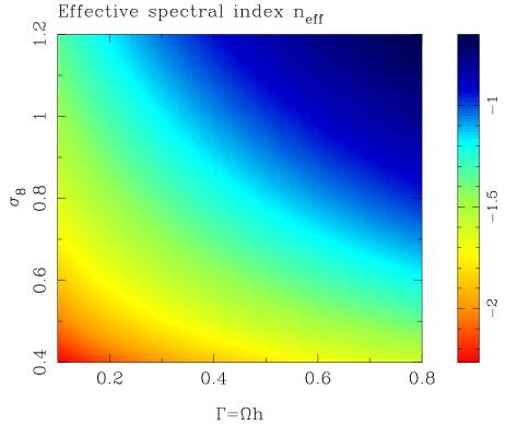
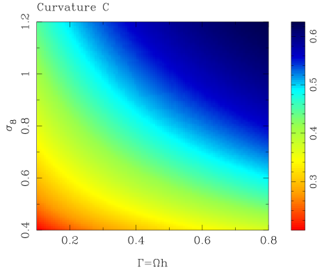
Fig. 10 shows the dependence of $k_{\sigma}$ (top panel), $n_{\rm eff}$ (middle panel) and $C$ (bottom panel) on the shape parameter and normalization of the linear power spectrum for $(0.1\leq\Gamma\leq 0.8)$ and $(0.4\leq\sigma_{8}\leq 1.2)$. In all of the models dark contrast represents a higher value. The parameters $n_{\rm eff}$ and $C$ are degenerate under $\Gamma$ and $\sigma_{8}$. This degeneracy is, however, broken by including the nonlinear wavenumber.

6.5 Parameter optimization

Figure 11: (Top) nonlinear power ratioed to the linear power as a function of wavenumber scaled in terms of the normalization wavenumber $k_{0}$: where $\Delta^{2}(k_{0})=1$. The data points are for the scale-free simulations; the solid lines represent the fits from the new halo based formula in Section 6.5; the dotted lines are PD96 fits. (Bottom) The goodness of the new fit. The $y$ axis represents the ratio of observed nonlinear power to nonlinear power predicted by the halo based fitting function. The $x$ axis is observed nonlinear power.

Figure 12: Top and bottom panels are similar to Fig. 11, but this time points represent open model data. Five epochs are shown; these are $a=0.6,0.7,0.8,0.9,1.0$. In terms of $\Omega$, these epochs correspond to: $\Omega=0.294,0.263,0.238,0.217,0.200$. The thick solid line represents the new halo-model based fitting to the scale-free data.

Figure 13: Top and bottom panels are similar to Fig. 11, but this time points represent $\Lambda$ model data. Four epochs are shown; these are $a=0.7,0.8,0.9,1.0$. In terms of $\Omega$, these epochs correspond to: $\Omega=0.505,0.407,0.325,0.260$. Again, the thick solid line represents the fit to the scale-free data.

We now give the best-fitting coefficients, including dependence on cosmology. These coefficients were obtained by optimizing the formula to fit the scale-free and $\Omega<1$ power-law simulations described here; the CDM simulations of J98; and on large scales ($k<0.15{\,h\,\rm Mpc^{-1}}$), the results of 2nd-order perturbation theory (calculated using the formulae of  ̵Lokas et al. 1996). Owing to the fact that numerical simulations are susceptible to sample variance on large scales, analytic perturbation theory results were preferred. In the halo model the cosmology dependence arises in a subtle way. To the extent that the mass function depends only on $\nu$ (when expressed as a function of $R$) and that $\delta_{c}$ has no strong cosmology dependence, the mass function for a given spectrum is also independent of cosmology. Therefore, the only effect on the halo power spectrum should be through the sizes of haloes; these depend on cosmology because haloes that collapse at high redshift are smaller. Collapse redshift is a function of mass and cosmology (see e.g. Appendix C of Peacock & Smith 2000). High-mass haloes always have $z_{c}\simeq 0$; these thus filter the large-scale part of the spectrum in a cosmology-independent way. Conversely, low-mass haloes are important at high $k$, and these do depend on cosmology – which alters the effective scale at which filtering occurs. However, there appears to be no simple way to implement such a complicated dependence into the fitting procedure. We therefore insert empirical functions of $\Omega$ into the procedure. Also, motivated by the findings of Section 5, we allowed the power-law indices that govern the quasi-linear regime to be density dependent.

The prescription that was found to work best is given in Appendix C. Code to evaluate the fitting function can be downloaded from the web address listed in the abstract. Note that the above coefficients were obtained by fitting the data over a restricted range of scales. The scale-free data were constrained to have $k/k_{\sigma}>0.3$. The open and $\Lambda$ data were constrained to lie in the range: $(4.0<\Delta^{2}_{\kern 0.35002pt{\scriptscriptstyle{\rm L}}}<15.0)$ for $n=-2$; $(0.3<\Delta^{2}_{\kern 0.35002pt{\scriptscriptstyle{\rm L}}}<15.0)$ for $n=-1.5$; $(0.3<\Delta^{2}_{\kern 0.35002pt{\scriptscriptstyle{\rm L}}}<20.0)$ for $n=-1$; $(0.3<\Delta^{2}_{\kern 0.35002pt{\scriptscriptstyle{\rm L}}}<25.0)$ for $n=0$. The CDM data were fit under the constraints: $k>0.3$ for the big box data and to $k>0.5{\,h\,\rm Mpc^{-1}}$ for the higher resolution small box calculations; the nonlinear power must be 10% greater than the discreteness correction, equation (38). On larger scales $k<0.15{\,h\,\rm Mpc^{-1}}$, the formula was calibrated to the results of 2nd-order perturbation theory.

In Fig. 11 we compare our new halo-based fitting function with the scale-free simulations. The new model clearly reproduces the data to a high degree of accuracy. Also, it is important to note that when the data are plotted in this way the scaling nature is again apparent and the departure from stable clustering, which is indicated by the deviation away from PD96 for $k/k_{0}>10$, is pronounced.

In Figs 12 and 13 we compare the new halo based model with the power-law data for $\Omega<1$ and $\Omega+\Lambda=1$. For all of the models the inclusion of the functions $f_{1}$, $f_{2}$ and $f_{3}$, seems to well reproduce the observed density-dependent growth. The only significant discrepancy is for the $n=-2$ open data, where the power is underpredicted in the quasi-linear regime.

In Figs 14 and 15 we compare the model with the CDM data. Again, the model does exceptionally well at reproducing all of the data over the range of scales where we are confident that numerical effects are unimportant. In particular, the OCDM and $\tau$CDM predictions are very significantly improved using the new prescription.

Figure 14: Power spectra for the four Virgo CDM simulations (J98) in large cosmological volumes, $L=239.5h^{-1}{\rm Mpc}$. Each panel shows the evolution of structure with redshift. The data points correspond, from low to high, to epochs $z=0,\;0.5,\;1.0,\;2.0$ and $3.0$. Note that only those points with a measured power above the discreteness spectrum are plotted. The solid line represents the new halo-model based fitting procedure, with dotted lines representing the decomposition into the self-halo and halo-halo terms; the dashed line is the PD96 fit.

Figure 15: Same as for Fig. 14, but this time for the smaller box GIF simulations.

Figure 16: Comparison to perturbation theory. The top panel shows the ratio of the evolved power to the linear power for two CDM models with $\Gamma=0.2$, but with different normalizations. The model with $\sigma_{8}=1.$ has been translated by a factor of 0.5 in the $y$-direction. The points represent perturbation theory; the thick solid line is this work; the dashed line represents PD96. The bottom panel is the same as the top, but with $\Gamma=0.5$.

Having demonstrated the success of the halo fitting function on small scales, we next consider the large scales. We assess this using the predictions derived from 2nd order perturbation theory (see Baugh & Efstathiou 1994). Fig. 16 shows the ratio of nonlinear to linear power for four CDM models. The current models match perturbation theory for $k<0.1{\,h\,\rm Mpc^{-1}}$, but deviations exist at higher $k$. These plausibly reflect a genuine breakdown of perturbation theory, since the model was required to match perturbation theory as well as possible for $k<0.15{\,h\,\rm Mpc^{-1}}$, and yet the fit is breaking down slightly before this upper limit. Both the halo fitting function and PD96 agree well in this range.

7 Conclusions and discussion

In this paper we have presented a set of high-resolution, $256^{3}$ particle, scale-free $N$-body simulations, designed to investigate self-similar gravitational clustering and in particular the effects of nonlinear evolution. We have also performed a further series of numerical simulations, with the same resolution, to explore how the evolution of clustering depends upon the background density of the universe. Together, these simulations represent the best calculations that exist to date for the set of models explored, with a factor 512 improvement in mass resolution over the ground-breaking work of Efstathiou et al. [1988].

We verified that the final output power spectra were robust by considering grid and glass particle loads. However, at early times the problem of discreteness correction is simpler to handle if a glass start is applied; we have described a detailed method for correcting the clustering signal in this case. We have implemented the power spectrum estimation technique of J98, which allowed us to probe high spatial frequencies without aliasing effects or errors due to mass assignment to the Fourier mesh. The simulation results may be summarized as follows:

1. Scale-free simulations with $0<n<-2$ show self-similarity under the scaling $k_{0}(a)\propto a^{-2/(n+3)}$. This conclusion is in agreement with the results of Efstathiou [1988] and Jain & Bertschinger [1998].

2. In the quasi-linear regime, the power spectrum is characterized by a steep power law. The exact slope depends upon the spectral index $n$ of the input spectrum and the value of $\Omega$, the slope steepening as $n$ becomes more negative and as $\Omega$ is reduced.

3. The observed nonlinear asymptote of the Einstein–de Sitter simulations was found to be inconsistent with the $\Delta_{\kern 0.35002pt{\scriptscriptstyle{\rm NL}}}^{2}\propto[\Delta_{\kern 0.35002pt{\scriptscriptstyle{\rm L}}}^{2}]^{3/2}$ prediction of stable clustering. A shallower slope with $\Delta_{\kern 0.35002pt{\scriptscriptstyle{\rm NL}}}^{2}\propto[\Delta_{\kern 0.35002pt{\scriptscriptstyle{\rm L}}}^{2}]^{1}$ is preferred. This result makes sense in terms of the halo model: calculations using the extended Press-Schechter apparatus show that haloes will tend to merge with systems of similar mass to their own [1993]. Mergers of this kind will disrupt the virial equilibrium of the system, violating the basic assumption that underlies stable clustering. However, if this process were rare then stable clustering could be upheld in a statistical sense.

4. The nonlinear fitting formulae of PD96 and JMW95 failed to reproduce the $n=-2$ results and were only marginally successful at reproducing the steeper spectra. The low-density power-law data were poorly fit by PD96.

5. For the $\Omega<1$ simulations, it is interesting to consider how the nonlinear slope changes with density. In the nonlinear limit equation (72) (appendix C) becomes

   $$\Delta^{2}(k)\propto k^{\;[3(f_{1}-1)+\gamma_{n}]}\ .$$ (61)

   For a given $n$, $f_{1}$ increases as $\Omega$ decreases, and so the power-law slope steepens. This result supports the idea that small scale clustering is more closely related to the emergence of the internal density structure through the continual accretion and merger of haloes. The reasoning is as follows: for a low-density universe mergers are less frequent and so haloes have more time to virialize. This means that stable clustering may be considered to be a better approximation for these systems. From the arguments in Section 1 and 5, this would then be manifest as a steepening of the nonlinear slope.

In the second part of this paper, we proposed an improved fitting function for mass power spectra to replace the much-used PD96 formula. We have adopted a new approach to fitting power spectra, based upon a fusion of the halo model and a HKLM scaling. The method was generalized to fit more realistic curved spectra, by introducing two new parameters, $n_{\rm eff}$ the effective spectral index on the nonlinear scale, and the spectral curvature, $C$. We found that the halo model as previously envisaged in the literature fails to approach linear theory on large scales for $n\geq 0$. We have argued that this should be cured by changing the self-halo power from $n=0$ to $n=2$ on large enough scales, and we have shown empirically that this approach allows an accurate description of a very wide range of power spectrum data. Our new fitting formula reproduced the scale-free power spectrum data and also the CDM results of J98 with an rms error better than 7%. This is to be preferred to the widely-used PD96 prescription, and should be useful for a variety of cosmological investigations. In particular, our preliminary investigations show that the present formalism should cope naturally with spectra containing a realistic degree of baryonic features (e.g. Meiksin, White & Peacock 1999).

The halo model provides a novel way to view structure formation, and has yielded useful insights into the origin of nonlinear aspects of galaxy clustering. This work has concentrated on the low-order statistics of the density field, but it is also possible to consider higher-order statistics such as the bispectrum. This three-point function in Fourier space probes the shapes of large-scale structures that are generated by gravitational clustering. No shape information is included in the current formalism, so it will be interesting to see how well the model can account for higher-order statistics. Initial results in this direction (Scoccimarro et al. 2001) seem to be promising. In general, the important question is the extent to which the halo model can encapsulate the phase information in the density field, since fields with identical power spectra can possess completely different real-space distributions (e.g. Chiang & Coles 2000). The halo model will inevitably fail to encompass these details of the density field in full, although it may still offer useful insights. However, at the two-point level, we have shown that the model is far more than an educational device, and it can be used as a tool for a high-precision description of the evolution of the dark-matter power spectrum.

Appendix A HKLM fitting functions

A.1 The JMW95 function

The JMW95 function was designed to model the $n$-dependence of the nonlinear evolution of scale-free power spectra. The formula was also used to model $\Omega=1$, CDM-like models through the adoption of an effective spectral index; see equation (14). JMW’s formula described their numerical data with an rms accuracy of 15-20%, but for our higher resolution scale-free data the fit is much worse, having an rms error of 56%. Their formula is

$$\frac{\Delta_{\kern 0.35002pt{\scriptscriptstyle{\rm NL}}}^{2}(k_{\kern 0.35002pt{\scriptscriptstyle{\rm NL}}})}{B(n)}=f_{\kern 0.35002pt{\scriptscriptstyle{\rm JMW}}}\left[\frac{\Delta_{\kern 0.35002pt{\scriptscriptstyle{\rm L}}}^{2}(k_{\kern 0.35002pt{\scriptscriptstyle{\rm L}}})}{B(n)}\right]\ ,$$ (62)

where $B(n)$ is a constant which depends upon the spectral index $n$ and where $f_{\kern 0.35002pt{\scriptscriptstyle{\rm JMW}}}(y)$ remains independent of $n$. The explicit forms are:

$$B(n)=\left(\frac{3+n}{3}\right)^{1.3}$$ (63)

and

$$f_{\kern 0.35002pt{\scriptscriptstyle{\rm JMW}}}(y)=y\left[\frac{1+0.6y+y^{2}-0.2y^{3}-1.5y^{3.5}+y^{4}}{1+0.0037y^{3}}\right]^{0.5}$$ (64)

where $y\equiv\Delta_{\kern 0.35002pt{\scriptscriptstyle{\rm L}}}^{2}(k_{\kern 0.35002pt{\scriptscriptstyle{\rm L}}})/B(n)$ .

A.2 The PD96 function

PD96 performed a similar study to JMW95, but extended the set of cosmological models to include $\Omega<1$ open and flat universes. They also improved on JMW95 by including CDM data in the optimization procedure and by proposing that the effective spectral index would vary continuously with scale: equation (15). They reported that their fitting formula described their simulation data to an accuracy of about 14%, but it describes our complete data set with an rms error of 54%. The PD96 fitting formula is

$$f_{\kern 0.35002pt{\scriptscriptstyle{\rm PD}}}(y)=y\left[\frac{1+B\beta y+[Ay]^{\alpha\beta}}{1+([Ay]^{\alpha}g^{3}(\Omega,\Lambda)/[Vy^{1/2}])^{\beta}}\right]^{1/\beta}\ ,$$ (65)

where $y\equiv\Delta_{\kern 0.35002pt{\scriptscriptstyle{\rm L}}}^{2}(k_{\kern 0.35002pt{\scriptscriptstyle{\rm L}}})$. $B$ describes a second order deviation from linear growth; $A$ and $\alpha$ parameterize the power law that dominates the function in the quasi-linear regime; $V$ is the virialization parameter that gives the amplitude of the $f_{\kern 0.35002pt{\scriptscriptstyle{\rm NL}}}\propto y^{3/2}$ asymptote; $\beta$ softens the transition between these regions; $g(\Omega)$ is the density dependent growth factor of [1992], which is the ratio of the linear growth factor to the expansion factor. This has the functional form

 

$${g(\Omega)}$$

  (66)

The best-fitting parameters were

$$A = 0.482\,(1+n/3)^{-0.947}$$

$$B = 0.226\,(1+n/3)^{-1.778}$$

$$\alpha = 3.310\,(1+n/3)^{-0.244}$$

$$\beta = 0.862\,(1+n/3)^{-0.287}$$

$$V = 11.55\,(1+n/3)^{-0.423}.$$ (67)

Appendix B New HKLM fits to the present data

We have performed a nonlinear least squares fitting to the individual scale-free loci (see Fig. 5) using a single formula. The individual fitting functions are accurate to $\simeq 9\%$. The formula is

$$f_{\rm EdS}(y)=y\left[\frac{1+y/a+(y/b)^{2}+(y/c)^{\alpha-1}}{1+(y/d)^{(\alpha-\beta)\gamma}}\right]^{1/\gamma}\ ,$$ (68)

where $y\equiv\Delta_{\kern 0.35002pt{\scriptscriptstyle{\rm L}}}^{2}(k_{\kern 0.35002pt{\scriptscriptstyle{\rm L}}})$ and the relevant parameters for each $n$ are presented below

$$\begin{array}[]{cccccccc}n&a&b&c&d&\alpha&\beta&\gamma\\ -2&3.138&0.358&0.527&0.940&8.247&0.508&0.330\\ -1.5&2.710&0.710&0.919&1.852&0.707&0.647&0.332\\ -1&10.37&1.115&1.403&2.873&6.655&0.697&0.366\\ 0&29.26&1.394&1.941&3.753&6.547&0.847&0.351\end{array}$$

Appendix C The halo model fitting function

The halo model decomposes the power into a sum of two contributions:

$$\Delta^{2}_{\kern 0.35002pt{\scriptscriptstyle{\rm NL}}}(k)=\Delta^{2}_{\kern 0.35002pt{\scriptscriptstyle{\rm Q}}}(k)+\Delta^{2}_{\kern 0.35002pt{\scriptscriptstyle{\rm H}}}(k).$$ (69)

These are given separately by

$$\Delta^{2}_{\kern 0.35002pt{\scriptscriptstyle{\rm Q}}}(k)=\Delta^{2}_{\kern 0.35002pt{\scriptscriptstyle{\rm L}}}(k)\left[\frac{(1+\Delta_{\kern 0.35002pt{\scriptscriptstyle{\rm L}}}^{2}(k))^{\beta_{n}}}{1+\alpha_{n}\Delta^{2}_{\kern 0.35002pt{\scriptscriptstyle{\rm L}}}(k)}\right]\exp{[-f(y)]};$$ (70)

where $y\equiv k/k_{\sigma}$ and $f(y)=y/4+y^{2}/8$; and

$$\Delta^{2}_{\kern 0.35002pt{\scriptscriptstyle{\rm H}}}(k)={\Delta^{2\ \prime}_{\kern 0.35002pt{\scriptscriptstyle{\rm H}}}(k)\over 1+\mu_{n}y^{-1}+\nu_{n}y^{-2}},$$ (71)

where

$$\Delta^{2\ \prime}_{\kern 0.35002pt{\scriptscriptstyle{\rm H}}}(k)=\frac{a_{n}\;y^{3f_{1}(\Omega)}}{1+b_{n}y^{f_{2}(\Omega)}+\left[c_{n}f_{3}(\Omega)\;y\right]^{3-\gamma_{n}}}$$ (72)

and $y\equiv k/k_{\sigma}$.

The parameters of the spectrum are defined via Gaussian filtering:

$$\sigma^{2}(R_{\rm G})\equiv\int\Delta^{2}_{\kern 0.35002pt{\scriptscriptstyle{\rm L}}}(k)\,\exp(-k^{2}R_{\rm G}^{2})\;d\ln k.$$ (73)

In these terms,

$$\sigma(k_{\sigma}^{-1})\equiv 1.$$ (74)

The effective index is

$$3+n_{\rm eff}\equiv-\left.{d\ln\sigma^{2}(R)\over d\ln R}\right|_{\sigma=1},$$ (75)

and the spectral curvature is

$$C\equiv-\left.{d^{2}\ln\sigma^{2}(R)\over d\ln R^{2}}\right|_{\sigma=1}.$$ (76)

Allowing $(a_{n},b_{n},c_{n},\gamma_{n},\alpha_{n},\beta_{n},\mu_{n},\nu_{n})$ to vary as a function of spectral properties, the following coefficients fit our simulation data and the CDM simulations of J98 to an rms precision of 8.6% (very much better than PD96). In particular, the model describes the $\Lambda$CDM data of J98 extremely well. For redshifts $z<3$, the deviation in power between model and the average of the large-box and small-box data from J98 is always less than 3% for $k<10{\,h\,\rm Mpc^{-1}}$. This represents a perfect fit with present knowledge, since the two datasets themselves can differ by at least this much. Note the use of terms up to $n^{4}$ in the fit for $a_{n}$; these are required in order to describe the rapid rise in amplitude of the halo term for $n<-2$. For less negative $n$, the higher-order terms are unimportant. The coefficients are:

$$\log_{10}a_{n}=1.4861+1.8369\;n+1.6762\;n^{2}+0.7940\;n^{3}$$

$$\hskip 42.67912pt+0.1670\;n^{4}-0.6206\;C\;;$$ (77)

$$\log_{10}b_{n}=0.9463+0.9466\;n+0.3084\;n^{2}-0.9400\;C\;;$$ (78)

$$\log_{10}c_{n}=-0.2807+0.6669\;n+0.3214\;n^{2}\;-0.0793\;C\;;$$ (79)

$$\gamma_{n}=0.8649+0.2989\;n+0.1631\;C\;;$$ (80)

$$\alpha_{n}=1.3884+0.3700\;n-0.1452\;n^{2}\;;$$ (81)

$$\beta_{n}=0.8291+0.9854\;n+0.3401\;n^{2}\;;$$ (82)

$$\log_{10}\mu_{n}=-3.5442+0.1908\;n\;;$$ (83)

$$\log_{10}\nu_{n}=0.9589+1.2857\;n\;;$$ (84)

and the $\Omega$ dependent functions are:

$$\left.\begin{array}[]{lll}f_{1a}(\Omega)&=&\Omega^{\;-0.0732}\\ f_{2a}(\Omega)&=&\Omega^{\;-0.1423}\\ f_{3a}(\Omega)&=&\Omega^{\;0.0725}\\ \end{array}\right\}\ \ \Omega\leq 1$$ (85)

$$\left.\begin{array}[]{lll}f_{1b}(\Omega)&=&\Omega^{\;-0.0307}\\ f_{2b}(\Omega)&=&\Omega^{\;-0.0585}\\ f_{3b}(\Omega)&=&\Omega^{\;0.0743}\\ \end{array}\right\}\ \ \Omega+\Lambda=1$$ (86)

For models in which $\Lambda$ is neither zero nor $1-\Omega$, we suggest interpolating the functions $f_{1}$ etc. linearly in $\Lambda$ between the open and flat cases.

References

- [1998] Bagla J., Engineer S., Padmanabhan T., 1998. ApJ, 495, 25.
- [1994] Baugh C.M., Efstathiou G., 1994. MNRAS, 270, 183.
- [1995] Baugh C.M., Gaztanaga E., Efstathiou G., 1995. MNRAS, 274, 1049.
- [2000] Benson A., Cole S., Baugh C.M., Frenk C., 2000. MNRAS, 311, 793.
- [2001] Bernardeau F., Colombi S., Gaztanaga E., Scoccimarro R., 2002. Physics Reports, 367, 1; astro-ph/0112551.
- [2001] Bode P., Ostriker J., Turok N., 2001. ApJ, 556, 93.
- [2001] Caldwell R.R., Juskiewicz R., Steinhardt P.J., Bouchet F.R., 2001. ApJ, 547, L93.
- [1992] Carroll S.M., Press W.H., Turner E.L., 1992. ARAA, 30, 499.
- [1995] Couchman H.M.P., Thomas P.A., Pearce F.R., 1995. ApJ, 452, 797.
- [2000] Colberg J. M., White S. D. M., Yoshida N., MacFarland T. J., Jenkins A., Frenk C. S., Pearce F. R., Evrard A. E., Couchman H. M. P., Efstathiou G., Peacock J. A., Thomas P. A., The Virgo Consortium, 2000. ApJ, 452, 797.
- [1996] Colombi S., Bouchet F. R., Hernquist L., 1996. ApJ, 465, 14.
- [2000] Chiang L., Coles P., 2000. MNRAS, 311, 809.
- [1977] Davis M., Peebles P.J.E., 1977. ApJ Suppl., 34, 425.
- [1985] Efstathiou G., Davis M., White S.D.M., Frenk C.S., 1985. ApJ Suppl., 57, 241.
- [1988] Efstathiou G., Frenk C.S., White S.D.M., Davis M., 1988. MNRAS, 235, 715.
- [1992] Efstathiou G., Bond J. R., White S.D.M., 1992. MNRAS, 258, 1.
- [2001] Fukushige T., Suto Y., 2001. ApJL, 557, L11.
- [1975] Gott J.R. III, Rees M.J., 1974. A&A, 45, 365.
- [1991] Hamilton A.J.S., Kumar P., Lu E., Matthews A., 1991. ApJ Lett., 374, L1. (HKLM).
- [1997] Jain B., 1997. MNRAS, 287, 687.
- [1998] Jain B., Bertschinger E., 1998. ApJ, 509, 517.
- [1995] Jain B., Mo H.J., White S.D.M., 1995. MNRAS, 276, L25. (JMW95).
- [1998] Jenkins A., Frenk C.S., Pearce F.R., Thomas P.A., Colberg J.M., White S.D.M., Couchman H.M.P., Peacock J.A., Efstathiou G., Nelson A.H., 1998. ApJ, 499, 20. (J98).
- [2001] Jenkins A., Frenk C.S., White S.D., Colberg J.M., Cole S., Evrard A.E., Yoshida N., 2001. MNRAS, 321, 372.
- [1998] Jing J., Mo H.J., Börner G., 1998. ApJ, 494, 1.
- [1993] Lacey C., Cole S., 1993. MNRAS, 262, 627.
- [1996] ̵Lokas E.L., Juskiewicz R., Bouchet F.R., Hivon E., 1996. ApJ, 467, 1.
- [2001] Kanekar N., Padmanabhan T., 2001. MNRAS, 324, 988.
- [1998] Macfarland T., Couchman H. M. P., Pearce F. R., Pichlmeier J., 1998. New Astronomy, 3, 687.
- [2000a] Ma C., Fry J.N., 2000a. ApJ, 543, 503.
- [2000b] Ma C., Fry J.N., 2000b. ApJ Lett., 538, L107.
- [1977] McClelland J., Silk J., 1977. ApJ, 216, 665.
- [1999] Meiksin A., White M., Peacock J.A., 1999. MNRAS, 304, 851
- [1996] Mo H.J., White S.D.M., 1996. MNRAS, 282, 347.
- [1997] Mo H.J., Jing Y.P., Börner G., 1997. MNRAS, 286, 979.
- [1997] Mo H.J., Jing Y.P., White S.D.M., 1997. MNRAS, 284, 189.
- [1999] Moore B., Ghigna S., Governato F., Lake G., Quinn T., Stadel J., Tozzi P., 1999. ApJ Lett., 524, L19.
- [1996] Navarro J.F., Frenk C.S., White S.D.M., 1996. ApJ, 462, 563.
- [1997] Navarro J.F., Frenk C.S., White S.D.M., 1997. ApJ, 490, 493.
- [1952] Neyman J., Scott E.L., 1952. ApJ, 116, 144.
- [1996] Padmanabhan, T. Cen, R. Ostriker, J. P. Summers, F. J., 1996. ApJ, 466, 604.
- [1996] Padmanabhan T., 1996. MNRAS, 278, L29.
- [1994] Peacock J.A., Dodds S.J., 1994. MNRAS, 267, 1020. (PD94).
- [1996] Peacock J.A., Dodds S.J., 1996. MNRAS, 280, L19. (PD96).
- [1991] Peacock J.A., Nicholson D., 1991. MNRAS, 253, 307.
- [2000] Peacock J.A., Smith R.E., 2000. MNRAS, 318, 1144.
- [1997] Pearce F.R., Couchman H.M.P., 1997. New Astronomy, 2, 411.
- [1974a] Peebles P.J.E., 1974a. ApJ Lett., 189, L51.
- [1974b] Peebles P.J.E., 1974b. Astron. Astrophys., 32, 197.
- [1980] Peebles P.J.E., 1980. ”The large-scale structure of the universe”, Princeton University Press, Princeton N.J.
- [1974] Press W.H., Schechter P., 1974. ApJ, 187, 425.
- [1991] Scherrer R.J., Bertschinger E., 1991. ApJ, 381, 349.
- [1996] Scoccimarro R., Frieman J., 1996. ApJ, 473, 620.
- [2001] Scoccimarro R., Sheth R.K., Hui L., Jain B., 2001. ApJ, 546, 20.
- [2002] Scoccimarro R., Sheth R.K., 2002. MNRAS, 329, 629S.
- [2000] Seljak U., 2000. MNRAS, 318, 203.
- [2002] Sheth R.K., Cooray A., 2002. astro-ph/0206508
- [1997] Sheth R.K., Jain B., 1997. MNRAS, 285, 231.
- [1999] Sheth R.K., Lemson G., 1999. MNRAS, 304, 767.
- [1999] Sheth R.K., Tormen G., 1999. MNRAS, 308, 119.
- [2000] Sheth R.K., Mo H-J., Tormen G., 2000. MNRAS, 323, 1.
- [1998] Smith C.C., Klypin A., Gross M.A.K., Primack J.R., Holtzman J., 1998. MNRAS, 297, 910.
- [2001] Van Waerbeke, L. Mellier Y.,Radovich M., Bertin E., Dantel-Fort M., McCracken H. J., Le Fèvre O., Foucaud S., Cuillandre J.-C., Erben T., Jain B., Schneider P., Bernardeau F., Fort B., 2001. A&A, 374, 757.
- [1993] White S.D.M., 1993. In: Cosmology and Large Scale Structure, Les Houches Session LX, 77.
- [2000] Yano T., Gouda N., 2000. ApJ, 539, 493.
- [1970] Zel’dovich Y.B., 1970. A&A, 5, 84.